Robust Gaussian Process Regression with a Student-t Likelihood
Pasi Jyl¨anki [email protected]
Department of Biomedical Engineering and Computational Science Aalto University School of Science
P.O. Box 12200 FI-00076 Aalto Finland
Jarno Vanhatalo [email protected]
Department of Environmental Sciences University of Helsinki
P.O. Box 65 FI-00014 Helsinki Finland
Aki Vehtari [email protected]
Department of Biomedical Engineering and Computational Science Aalto University School of Science
P.O. Box 12200 FI-00076 Aalto Finland
Editor: Neil Lawrence
Abstract
This paper considers the robust and efficient implementation of Gaussian process regression with a Student-t observation model, which has a non-log-concave likelihood. The challenge with the Student-t model is the analytically intractable inference which is why several approximative meth-ods have been proposed. Expectation propagation (EP) has been found to be a very accurate method in many empirical studies but the convergence of EP is known to be problematic with models con-taining non-log-concave site functions. In this paper we illustrate the situations where standard EP fails to converge and review different modifications and alternative algorithms for improving the convergence. We demonstrate that convergence problems may occur during the type-II maximum a posteriori (MAP) estimation of the hyperparameters and show that standard EP may not converge in the MAP values with some difficult data sets. We present a robust implementation which relies primarily on parallel EP updates and uses a moment-matching-based double-loop algorithm with adaptively selected step size in difficult cases. The predictive performance of EP is compared with Laplace, variational Bayes, and Markov chain Monte Carlo approximations.
Keywords: Gaussian process, robust regression, Student-t distribution, approximate inference, expectation propagation
1. Introduction
measurement process or absence of certain relevant explanatory variables in the model. In such cases, a robust observation model is required.
Robust inference has been studied extensively. De Finetti (1961) described how Bayesian in-ference on the mean of a random sample, assuming a suitable observation model, naturally leads to giving less weight to outlying observations. However, in contrast to simple rejection of outliers, the posterior depends on all data but in the limit, as the separation between the outliers and the rest of the data increases, the effect of outliers becomes negligible. More theoretical results on this kind of outlier rejection were presented by Dawid (1973) who gave sufficient conditions on the observation
model p(y|θ)and the prior distribution p(θ)of an unknown location parameterθ, which ensure that
the posterior expectation of a given function m(θ)tends to the prior as y→∞. He also stated that
the Student-t distribution combined with a normal prior has this property.
A more formal definition of robustness was given by O’Hagan (1979) in terms of an outlier-prone observation model. The observation model is defined to be outlier-outlier-prone of order n, if
p(θ|y1, ...,yn+1)→ p(θ|y1, ...,yn) as yn+1 →∞. That is, the effect of a single conflicting
obser-vation to the posterior becomes asymptotically negligible as the obserobser-vation approaches infinity. O’Hagan (1979) showed that the Student-t distribution is outlier prone of order 1, and that it can reject up to m outliers if there are at least 2m observations altogether. This contrasts heavily with the commonly used Gaussian observation model in which each observation influences the posterior no matter how far it is from the others.
In nonlinear Gaussian process (GP) regression context the outlier rejection is more complicated
and one may consider the posterior distribution of the unknown function values fi= f(xi)locally
near some input locations xi. Depending on the smoothness properties defined through the prior
on fi, m observations can be rejected locally if there are at least 2m data points nearby. However,
already two conflicting data points can render the posterior distribution multimodal making the posterior inference challenging (these issues will be illustrated in the upcoming sections).
In this work, we adopt the Student-t observation model for GP regression because of its good robustness properties which can be altered continuously from a very heavy tailed distribution to the Gaussian model with the degrees of freedom parameter. This allows the extent of robustness to be determined from the data through hyperparameter inference. The Student-t observation model was studied in linear regression by West (1984) and Geweke (1993), and Neal (1997) introduced it for GP regression. Other robust observation models which have been used in GP regression include, for example, mixtures of Gaussians (Kuss, 2006; Stegle et al., 2008), the Laplace distribution (Kuss, 2006), and input dependent observation models (Goldberg et al., 1998; Naish-Guzman and Holden, 2008).
(see Nickisch and Rasmussen, 2008, for details and comparisons in GP classification). Yet an-other related variational approach is described by Opper and Archambeau (2009) who studied the Cauchy observation model (Student-t with degrees of freedom 1). This method is similar to the KL-divergence minimization approach (KL) described by Nickisch and Rasmussen (2008) and the VB approach can be regarded as a special case of KL. The extensive comparisons by Nickisch and Rasmussen (2008) in GP classification suggest that VB provides better predictive performance than the Laplace approximation but worse marginal likelihood estimates than KL or expectation propa-gation (EP) (Minka, 2001a). According to the comparisons of Nickisch and Rasmussen (2008), EP is the method of choice since it is much faster than KL, at least in GP classification. The problem with EP, however, is that the Student-t likelihood is not log-concave which may lead to convergence problems (Seeger, 2008).
In this paper, we focus on establishing a robust EP implementation for the Student-t observa-tion model. We illustrate the convergence problems of standard EP with simple one-dimensional regression examples and discuss how damping, fractional EP updates (or power EP) (Minka, 2004; Seeger, 2005), and double-loop algorithms (Heskes and Zoeter, 2002) can be used to improve the convergence. We present a robust implementation which relies primarily on parallel EP updates (see, e.g., van Gerven et al., 2009) and uses a moment-matching-based double-loop algorithm with adaptively selected step size to find stationary solutions in difficult cases. We show that the imple-mentation enables a robust type-II maximum a posteriori (MAP) estimation of the hyperparameters based on the approximative marginal likelihood. The proposed implementation is general so that it could be applied also to other models having non-log-concave likelihoods. The predictive perfor-mance of EP is compared to the Laplace approximation, fVB, VB, and Markov chain Monte Carlo (MCMC) using one simulated and three real-world data sets.
2. Gaussian Process Regression with the Student-t Observation Model
We will consider a regression problem, with scalar observations yi = f(xi) +εi,i=1, ...,n at
in-put locations X={xi}ni=1, and where the observation errorsε1, ...,εnare zero-mean exchangeable
random variables. The object of inference is the latent function f(x):ℜd →ℜ, which is given a
Gaussian process prior
f(x)|θ∼
GP
m(x),k(x,x′|θ), (1)
where m(x)and k(x,x′|θ)are the mean and covariance functions of the process controlled by
hyper-parametersθ. For notational simplicity we will assume a zero mean GP. By definition, a Gaussian
process prior implies that any finite subset of latent variables, f={f(xi)}ni=1, has a multivariate
Gaussian distribution. In particular, at the observed input locations X the latent variables are dis-tributed as p(f|X,θ) =
N
(f|0,K), where K is the covariance matrix with entries Ki j=k(xi,xj|θ). The covariance function encodes the prior assumptions on the latent function, such as the smooth-ness and scale of the variation, and can be chosen freely as long as the covariance matrices which it produces are symmetric and positive semi-definite. An example of a stationary covariance function is the squared exponentialkse(xi,xj|θ) =σ2seexp −
d
∑
k=1
(xi,k−xj,k)2 2lk2
!
whereθ={σ2
se,l1, ...,ld},σ2seis a magnitude parameter which scales the overall variation of the
un-known function, and lkis a length-scale parameter which governs how fast the correlation decreases
as the distance increases in the input dimension k.
The traditional assumption is that given f the error termsεiare i.i.d. Gaussian: εi∼
N
(0,σ2). Inthis case, the marginal likelihood p(y|X,θ,σ2)and the conditional posterior of the latent variables
p(f|
D
,θ,σ2), whereD
={y,X}, have an analytical solution. This is computationally convenientsince approximate methods are needed only for the inference on the hyperparametersθandσ2. The
robust Student-t observation model
p(yi|fi,σ2,ν) =
Γ((ν+1)/2) Γ(ν/2)√νπσ
1+(yi−fi) 2 νσ2
−(ν+1)/2
,
where fi = f(xi),νis the degrees of freedom andσthe scale parameter (Gelman et al., 2004), is
computationally challenging. The marginal likelihood and the conditional posterior p(f|
D
,θ,σ2,ν)are not anymore analytically tractable but require some method for approximate inference.
3. Approximate Inference
In this section, we review the approximate inference methods considered in this paper. First we give a short description of MCMC and the Laplace approximation, as well as two variational methods, fVB and VB. Then we give a more detailed description of the EP algorithm and review ways to improve the convergence in more difficult problems.
3.1 Markov Chain Monte Carlo
The MCMC approach is based on drawing samples from p(f,θ,σ2,ν|
D
)and using these samples torepresent the posterior distribution and to numerically approximate integrals over the latent variables and the hyperparameters. Instead of implementing a Markov chain sampler directly for the Student-t model, a more common approach is to use the Gibbs sampling based on the following scale mixture representation of the Student-t distribution
yi|fi,Vi∼
N
(fi,Vi),Vi|ν,σ2∼Inv-χ2(ν,σ2), (3)
where each observation has its own Inv-χ2-distributed noise variance Vi (Neal, 1997; Gelman et al.,
2004). Sampling of the hyperparametersθcan be done with any general sampling algorithm, such
as the Slice sampling or the hybrid Monte Carlo (HMC) (see, e.g., Gelman et al., 2004). The Gibbs sampler on the scale mixture (3) converges often slowly and may get stuck for long times
in small values of σ2 because of the dependence between Vi andσ2. This can be avoided by
re-parameterization Vi=α2Ui, where Ui ∼Inv-χ2(ν,τ2), p(τ2)∝1/τ2, and p(α2)∝1/α2 (Gelman
et al., 2004). This improves mixing of the chains and reduces the autocorrelations but introduces
an implicit prior for the scale parameterσ2=α2τ2of the Student-t model. An alternative
param-eterization proposed by Liu and Rubin (1995), where Vi=σ2/γi andγi∼Gamma(ν/2,ν/2), also
decouplesσ2 and V
i but does not introduce the additional scale parameter τ. It could also lead to
better mixing without the implicit scale prior but in the experiments we used the decomposition of
3.2 Laplace Approximation (LA)
The Laplace approximation for the conditional posterior of the latent function is constructed from
the second order Taylor expansion of log p(f|
D
,θ,σ2,ν)around the mode ˆf, which gives a Gaussianapproximation to the conditional posterior
p(f|
D
,θ,σ2,ν)≈q(f|D
,θ,σ2,ν) =N
(f|ˆf,ΣLA),where ˆf=arg maxfp(f|
D
,θ,σ2,ν) (Rasmussen and Williams, 2006). Σ−1LA is the Hessian of the
negative log conditional posterior at the mode, that is,
Σ−LA1=−∇∇log p(f|
D
,θ,σ2,ν)|f=ˆf=K−1+W, (4)where W is a diagonal matrix with entries Wii=∇fi∇filog p(y|fi,σ
2,ν)|
fi=fˆi.
The inference in the hyperparameters is done by approximating the conditional marginal
likeli-hood p(y|X,θ,σ2,ν)with Laplace’s method and searching for the approximate maximum a
poste-rior estimate for the hyperparameters
{θˆ,σˆ2,νˆ}=arg max θ,σ2,ν
log q(θ,σ2,ν|
D
)=arg max
θ,σ2,ν
log q(y|X,θ,σ2,ν) +log p(θ,σ2,ν)
,
where p(θ,σ2,ν)is the prior of the hyperparameters. The gradients of the approximate log marginal
likelihood can be solved analytically, which enables the MAP estimation of the hyperparameters with gradient based optimization methods. Following Williams and Barber (1998) the approxima-tion scheme is called the Laplace method, but essentially the same approach is named Gaussian approximation by Rue et al. (2009) in their Integrated nested Laplace approximation (INLA) soft-ware package for Gaussian Markov random field models (Vanhatalo et al., 2009), (see also Tierney and Kadane, 1986).
The implementation of the Laplace algorithm for this particular model requires care since the
Student-t likelihood is not log-concave and thus p(f|
D
,θ,σ2,ν) may be multimodal and some ofthe Wiinegative. It follows that the standard implementation presented by Rasmussen and Williams
(2006) requires some modifications in determining the mode ˆf and the covarianceΣLA which are
discussed in detail by Vanhatalo et al. (2009). Later on Hannes Nickisch proposed a slightly dif-ferent implementation (personal communication) where the stabilized Newton algorithm is used for
finding ˆf instead of the EM algorithm and LU decomposition for determiningΣLAinstead of rank-1
Cholesky updates (see also Section 4.1). This alternative approach is used at the moment in the GPML software package (Rasmussen and Nickisch, 2010).
3.3 Factorizing Variational Approximation (fVB)
The scale-mixture decomposition (3) enables a computationally convenient variational
approxima-tion if the latent values f and the residual variance terms V= [V1, ...,Vn]are assumed a posteriori
independent:
q(f,V) =q(f)
n
∏
i=1
q(Vi). (5)
(2006) and essentially the same variational approach has also been used for approximate inference on linear models with the automatic relevance determination prior (see, e.g., Tipping and Lawrence,
2005). Assuming the factorizing posterior (5) and minimizing the KL-divergence from q(f,V)to
the true posterior p(f,V|
D
,θ,σ2,ν)results in a Gaussian approximation for the latent values, andinverse-χ2(or equivalently inverse gamma) approximations for the residual variances Vi. The
param-eters of q(f)and q(Vi)can be estimated by maximizing a variational lower bound for the marginal
likelihood p(y|X,θ,σ2,ν)with an expectation maximization (EM) algorithm. In the E-step of the
algorithm the lower bound is maximized with respect to q(f)and q(Vi)given the current point
esti-mate of the hyperparameters and in the M-step a new estiesti-mate of the hyperparameters is determined with fixed q(f)and q(Vi).
The drawback with a factorizing approximation determined by minimizing the reverse KL-divergence is that it tends to underestimate the posterior uncertainties (see, e.g., Bishop, 2006). Vanhatalo et al. (2009) compared fVB with the previously described Laplace and MCMC approxi-mations, and found that fVB provided worse predictive variance estimates compared to the Laplace
approximation. In addition, the estimation ofνbased on maximizing the variational lower bound
was found less robust with fVB.
3.4 Variational Bounds (VB)
This variational bounding method was introduced for binary GP classification by Gibbs and MacKay (2000) and comparisons to other approximative methods for GP classification were done by Nick-isch and Rasmussen (2008). The method is based on forming a Gaussian lower bound for each likelihood term independently:
p(yi|fi)≥exp(−fi2/(2γi) +bifi−h(γi)/2),
which can be used to construct a lower bound on the marginal likelihood: p(y|X,θ,ν,σ)≥ZVB.
With fixed hyperparameters, γi and bi can be determined by maximizing ZVB to obtain a
Gaus-sian approximation for p(f|
D
,θ,ν,σ2)and an approximation for the marginal likelihood. With theStudent-t observation model only the scale parametersγi need to be optimized because the location
parameter is determined by the corresponding observations: bi=yi/γi. Similarly to the Laplace
ap-proximation and EP, MAP-estimation of the hyperparameters can be done by optimizing ZVBwith
gradient-based methods. In our experiments we used the implementation available in the GPML-package (Rasmussen and Nickisch, 2010) augmented with the same hyperprior definitions as with the other approximative methods.
3.5 Expectation Propagation
The EP algorithm is a general method for approximating integrals over functions that factor into simple terms (Minka, 2001a). It approximates the conditional posterior with
q(f|
D
,θ,σ2,ν) = 1ZEP
p(f|θ)
n
∏
i=1
˜ti(fi|Z˜i,˜µi,σ˜2i) =
N
(µ,Σ), (6)where ZEP≈p(y|X,θ,σ2,ν), and the parameters of the approximate conditional posterior
distribu-tion are given byΣ= (K−1+Σ˜−1)−1,µ=ΣΣ˜−1µ˜, ˜Σ=diag[σ˜2
1, ...,σ˜2n], and ˜µ= [˜µ1, ...,˜µn]T. In
Equation (6) the likelihood terms p(yi|fi,σ2,ν)are approximated by un-normalized Gaussian site
The EP algorithm updates the site parameters ˜Zi, ˜µiand ˜σ2i and the posterior approximation (6) sequentially. At each iteration (i), first the i’th site is removed from the i’th marginal posterior to obtain a cavity distribution
q−i(fi)∝q(fi|
D
,θ,σ2,ν)˜ti(fi)−1.Then the i’th site is replaced with the exact likelihood term to form a tilted distribution ˆpi(fi) =
ˆ
Zi−1q−i(fi)p(yi|fi) which is a more refined non-Gaussian approximation to the true i’th marginal
distribution. Next the algorithm attempts to match the approximative posterior marginal q(fi) =
q(fi|
D
,θ,σ2,ν)with ˆpi(fi)by finding first a Gaussian ˆqi(fi)satisfying ˆqi(fi) =
N
(fi|ˆµi,σˆ2i) =arg min qiKL(pˆi(fi)||qi(fi)),
which is equivalent to matching ˆµiand ˆσ2i with the mean and variance of ˆpi(fi). Then the parameters
of the local approximation ˜ti are updated so that the moments of q(fi)match with ˆqi(fi):
q(fi|
D
,θ,σ2,ν)∝q−i(fi)˜ti(fi)≡ZˆiN
(fi|ˆµi,σˆ2i). (7)Finally, the parameters µ and Σ of the approximate posterior (6) are updated according to the
changes in site ˜ti. These steps are repeated for all the sites at some order until convergence.
Since only the means and variances are needed in the Gaussian moment matching only ˜µi and
˜
σ2
i need to be updated during the iterations. The normalization terms ˜Zi are required for the
marginal likelihood approximation ZEP ≈ p(y|X,θ,σ2,ν) which is computed after convergence
of the algorithm, and they can be determined by integrating over fi in Equation (7) which gives
˜
Zi=Zˆi(
R
q−i(fi)
N
(fi|˜µi,σ˜2i)d fi)−1.In the traditional EP algorithm (from now on referred to as sequential EP), the posterior
approx-imation (6) is updated sequentially after each moment matching(7). Recently an alternative parallel
update scheme has been used especially in models with a very large number of unknowns (see, e.g., van Gerven et al., 2009). In parallel EP the site updates are calculated with fixed posterior marginals
µand diag(Σ)for all ˜ti, i=1, ...,n, in parallel, and the posterior approximation is refreshed only
after all the sites have been updated. Although the theoretical cost for one sweep over the sites is
the same (
O
(n3)) for both sequential and parallel EP, in practice one re-computation ofΣusing theCholesky decomposition is much more efficient than n sequential rank-one updates. In our exper-iments, the number of sweeps required for convergence was roughly the same for both schemes in easier cases where standard EP converges.
The marginal likelihood approximation is given by
log ZEP=−
1
2log|K+Σ˜| − 1 2µ˜
T K+ ˜
Σ−1µ˜+
n
∑
i=1
log ˆZi(σ2,ν) +CEP, (8)
where CEP=−n2log(2π)−∑ilog
R
q−i(fi)
N
(fi|˜µi,σ˜2i)d fi collects terms that are not explicitfunc-tions ofθ,σ2orν. If the algorithm has converged, that is, ˆpi(fi)is consistent (has the same means
and variances) with q(fi)for all sites, CEP, ˜Σand ˜µcan be considered constants when
differentiat-ing (8) with respect to the hyperparameters (Seeger, 2005; Opper and Winther, 2005). This enables efficient MAP estimation with gradient based optimization methods.
fine in many cases (see, e.g., Nickisch and Rasmussen, 2008). However, in case of a non-log-concave likelihood such as the Student-t likelihood, convergence problems may arise and these will be discussed in Section 5. The convergence can be improved either by damping the EP updates (Minka and Lafferty, 2002) or by using a robust but slower double-loop algorithm (Heskes and
Zoeter, 2002). In damping, the site parameters in their natural exponential forms, ˜τi=σ˜−i 2 and
˜
νi=σ˜−i 2˜µi, are updated to a convex combination of the old and proposed new values, which results
in the following update rules:
∆τ˜i=δ(σˆi−2−σ−i 2) and ∆ν˜i=δ(σˆ−i 2ˆµi−σ−i 2µi), (9)
where µiandσ2i are the mean and variance of q(fi|
D
,θ,σ2,ν), andδ∈(0,1]is a step size parametercontrolling the amount of damping. Damping can be viewed as using a smaller step size within a gradient-based search for saddle points of the same objective function as is used in the double-loop algorithm (Heskes and Zoeter, 2002).
3.6 Expectation Propagation, the Double-Loop Algorithm
When either sequential or parallel EP does not converge one may still find approximations satisfying the moment matching conditions (7) by a double loop algorithm. For example, Heskes and Zoeter (2002) present simulation results with linear dynamical systems where the double loop algorithm is able to find useful approximations when damped EP fails to converge. For the model under con-sideration, the fixed points of the EP algorithm correspond to the stationary points of the following objective function (Minka, 2001b; Opper and Winther, 2005)
min λs maxλ− −
n
∑
i=1
log Z
p(yi|fi)exp
ν−ifi−τ−i
fi2
2
d fi−log
Z p(f)
n
∏
i=1
exp
˜
νifi−τ˜i
fi2
2 df + n
∑
i=1
log Z
exp
νsifi−τsi
fi2
2
d fi (10)
where λ−={ν−i,τ−i}, ˜λ={ν˜i,τ˜i}, and λs={νsi,τsi} are the natural parameters of the cavity
distributions q−i(fi), the site approximations ˜ti(fi), and approximate marginal distributions qsi(fi) =
N
(τ−1si νsi,τ− 1
si ) respectively. The min-max problem needs to be solved subject to the constraints
˜
νi=νsi−ν−i and ˜τi =τsi−τ−i, which resemble the moment matching conditions in (7). The
objective function in (10) is equal to−log ZEPdefined in (6) and is also equivalent to the expectation
consistent (EC) free energy approximation presented by Opper and Winther (2005). A unifying view of the EC and EP approximations as well as the connection to the Bethe free energies is presented by Heskes et al. (2005).
Equation (10) suggests a double-loop algorithm where the inner loop consist of maximization
with respect toλ− with fixedλsand the outer loop of minimization with respect toλs. The inner
maximization affects only the first two terms and ensures that the marginal moments of the current
posterior approximation q(f)are equal to the moments of the tilted distributions ˆpi(fi)for fixedλs.
The outer minimization ensures that the moments qsi(fi)are equal to marginal moments of q(f). At
the convergence, q(fi), ˆpi(fi), and qsi(fi)share the same moments up to the second order. If p(yi|fi)
Since the first two terms in (10) are concave functions of λ− and ˜λ the inner maximization
problem is concave with respect toλ− (or equivalently ˜λ) after substitution of the constraints ˜λ=
λsi−λ− (Opper and Winther, 2005). The Hessian of the first term with respect toλ− is well
defined (and negative semi-definite) only if the tilted distributions ˆpi(fi)∝p(yi|fi)q−i(fi)are proper probability distributions with finite moments up to the fourth order. Therefore, to ensure that the
product of q−i(fi)and the Student-t site p(yi|fi)has finite moments and that the inner-loop moment
matching remains meaningful, the cavity precisionsτ−ihave to be kept positive. Furthermore, since
the cavity distributions can be regarded as estimates for the leave-one-out (LOO) distributions of
the latent values,τ−i=0 would correspond to a situation where q(fi|y−i,X)has infinite variance,
which does not make sense given the Gaussian prior assumption (1). On the other hand, ˜τi may
become negative for example when the corresponding observation yiis an outlier (see Section 5).
3.7 Fractional EP Updates
Fractional EP (or power EP, Minka, 2004) is an extension of EP which can be used to reduce the computational complexity of the algorithm by simplifying the tilted moment evaluations and to im-prove the robustness of the algorithm when the approximation family is not flexible enough (Minka, 2005) or when the propagation of information is difficult due to vague prior information (Seeger, 2008). In fractional EP the cavity distributions are defined as q−i(fi)∝q(fi|
D
,θ,ν,σ2)/˜ti(fi)η and the tilted distribution as ˆpi(fi)∝q−i(fi)p(yi|fi)η for a fraction parameterη∈(0,1]. The site parameters are updated so that the moments of q−i(fi)˜ti(fi)η∝q(fi)match with q−i(fi)p(yi|fi)η.Otherwise the procedure is similar and standard EP can be recovered by settingη=1. In fractional
EP the natural parameters of the cavity distribution are given by
τ−i=σ−i 2−ητ˜i and ν−i=σ−i 2µi−ην˜i, (11)
and the site updates (with damping factorδ) by
∆τ˜i=δη−1(σˆi−2−σ−i 2) and ∆ν˜i=δη−1(σˆi−2ˆµi−σ−i 2µi). (12)
The fractional update step minqKL(pˆi(fi)||q(fi)) can be viewed as minimization of the α
-divergence withα=η(Minka, 2005). Compared to the KL-divergence, minimizing theα-divergence
with 0<α<1 does not force q(fi) to cover as much of the probability mass of ˆpi(fi)whenever
ˆ
pi(fi)>0. As a consequence, fractional EP tends to underestimate the variance and normalization
constant of q−i(fi)p(yi|fi)η, and also the approximate marginal likelihood ZEP. On the other hand,
we also found that minimizing the KL-divergence in standard EP may overestimate the marginal likelihood with some data sets. In case of multiple modes, the approximation tries to represent the
overall uncertainty in ˆpi(fi)the more exactly the closerαis to 1. In the limitα→0 the reverse
KL-divergence is obtained which is used in some form, for example, in the fVB and KL approximations (Nickisch and Rasmussen, 2008). Also the double-loop objective function (10) can be modified according to the different divergence measure of fractional EP (Cseke and Heskes, 2011; Seeger and Nickisch, 2011).
Fractional EP has some benefits over standard EP with the non-log-concave Student-t sites.
First, when evaluating the moments of q−i(fi)p(yi|fi)η, settingη<1 flattens the likelihood term
cases are considered by Minka (2005). Second, the fractional updates help to avoid the cavity
preci-sions becoming too small, or even negative. Equation (11) shows that by choosingη<1, a fraction
(1−η) of the precision ˜τi of the i:th site is left in the cavity. This decreases the cavity variances
which in turn makes the tilted moment integrations and the subsequent EP updates (12) more ro-bust. Problems related to cavity precision becoming too small can be present also with log-concave sites when the prior information is vague. For example, Seeger (2008) reports that with an under-determined linear model combined with a log-concave Laplace prior the cavity precisions remain positive but they may become very small which induces numerical inaccuracies in the analytical moment evaluations. These inaccuracies may accumulate and even cause convergence problems. Seeger (2008) reports that fractional updates improve numerical robustness and convergence in such cases.
4. Robust Implementation of the Parallel EP Algorithm
The sequential EP updates are shown to be stable for models in which the exact site terms (in
our case the likelihood functions p(yi|fi)) are log-concave (Seeger, 2008). In this case, all site
variances, if initialized to non-negative values, remain non-negative during the updates. It follows
that the variances of the cavity distributions q−i(fi)are positive and thus also the subsequent moment
evaluations of q−i(fi)p(yi|fi)are numerically robust. The non-log-concave Student-t likelihood is
problematic because both the conditional posterior p(f|
D
,θ,ν,σ)as well as the tilted distributionsˆ
pi(fi) may become multimodal. Therefore extra care is needed in the implementation and these
issues are discussed in this section.
The double-loop algorithm is a rigorous approach that is guaranteed to converge to a stationary
point of the objective function (10) when the site terms p(yi|fi) are bounded from below. The
downside is that the double-loop algorithm can be much slower than for example parallel EP because it spends much computational effort during the inner loop iterations, especially in the early stages
when qsi(fi)are poor approximations for the true marginals. An obvious improvement would be to
start with damped parallel updates and to continue with the double-loop method if necessary. Since in our experiments parallel EP has proven quite efficient with many easier data sets, we adopt this approach and propose few modifications to improve the convergence in difficult cases. A parallel EP initialization and a double-loop backup is also used by Seeger and Nickisch (2011) in their fast EP algorithm.
Parallel EP can also be interpreted as a variant of the double-loop algorithm where only one inner-loop optimization step is done by moment matching (7) and each such update is followed by
an outer-loop refinement of the marginal approximations qsi(fi). The inner-loop step consists of
evaluating the tilted moments{ˆµi,σˆ2i|i=1, ...,n}with qsi(fi) =q(fi) =
N
(µi,Σii), updating thesites (9), and updating the posterior (6). The outer-loop step consists of setting qsi(fi) equal to
the new marginal distributions q(fi). Connections between the message passing updates and the
double-loop methods together with considerations of different search directions for the inner-loop optimization can be found in the extended version of Heskes and Zoeter (2002). The robustness of parallel EP can be improved by the following modifications.
1. After each moment matching step check that the objective (10) increases. If the objective does
not increase, decrease the damping coefficientδuntil increase is obtained. The downside is
but if these one-dimensional integrals are implemented efficiently this is a reasonable price for stability.
2. Before updating the sites (9) check that the new cavity variances τ−i =τsi−(τ˜i+∆τ˜i) are
positive. If they are negative, choose a smaller damping factorδso thatτ−i>0. This
com-putationally cheap precaution ensures that the increase of the objective (10) can be verified according to modification 1.
3. With modifications 1 and 2 the site parameters can still oscillate (see Section 5 for an illustra-tion) but according to our experiments the convergence is obtained with all hyperparameters
values eventually. The oscillations can be reduced by updating qsi(fi)only after the moments
of ˆpi(fi) and q(fi) are consistent for all i=1, ...,n with some small tolerance, for example
10−4. At each update, check also that the new cavity precisions are positive, and if not,
con-tinue the inner-loop iterations with the previous qsi(fi) until better moment consistency is
achieved or switch to fractional updates. Actually, this modification corresponds to the max-imization in (10) and it results in a double-loop algorithm where the inner-loop optmax-imization is done by moment matching (7). If no parallel initialization is done, often during the first
5-10 iterations when the step sizeδ is limited according to modification 2, the consistency
between ˆpi(fi)and q(fi)cannot be achieved. This is an indication of q(f)being a too
inflex-ible approximation for the tilted distributions with the current qsi(fi). An outer-loop update
qsi(fi) =q(fi)usually helps in these cases.
4. If sufficient increase of the objective is not achieved after an inner-loop update (modification
1), use the gradient information to obtain a better step sizeδ. The gradients of (10) with
respect to the site parameters ˜νi and ˜τi can be calculated without additional evaluations of
the objective function for fixedλs. With these gradients, it is possible to determine g(δ), the
gradient of the inner-loop objective function with respect toδin the current search direction.
For parallel EP the search direction is defined by (9) with fixed site updates∆τ˜i=σˆ−i 2−σ−i 2
and∆ν˜i=σˆ−i 2ˆµi−σ−i 2µi for i=1, ...,n. In case of a too large step, g(δ)becomes negative. Then, for example, spline interpolation with derivative constraints at the end points can be
used to approximate the objective as a function ofδ. From this approximation a better estimate
for the step sizeδ can be determined efficiently. In case of a too short step, g(δ) becomes
positive and a better step size can be obtained by extrapolating with constraints based on approximate second order derivatives. This modification corresponds to an approximative line search in the concave inner-loop maximization.
In the comparisons of Section 6 we start with 10 damped (δ=0.8) parallel iterations because
with a sensible hyperparameter initialization this is enough to achieve convergence in most hyper-parameter optimization steps with the empirical data sets. If no convergence is achieved this parallel initialization also speeds up the convergence of the subsequent double-loop iterations (see Section
5.3). If after any of the initial parallel updates the posterior covarianceΣbecomes ill-conditioned,
that is, many of the ˜τiare too negative, or any of the cavity variances become negative we reject the
frequent outer loop refinements of qsi(fi) were found to require fewer computationally expensive
objective evaluations for convergence.
In some rare cases, for example, when the noise levelσis very small, the outer-loop update of
qsi(fi)may result in negative values for some of the cavity variances even though the inner-loop
optimality is satisfied. In practise this means that [Σii]−1 is smaller than ˜τi for some i. This may
be a numerical problem or an indication of a too inflexible approximating family but switching to fractional updates helps. However, in our experiments, this happened only when the noise level was set to too small values and with a sensible hyperparameter initialization such problems did not emerge.
4.1 Other Implementation Details
The EP updates require evaluation of moments mk=
R
fikgi(fi)d fi for k=0,1,2, where we have defined gi(fi) =q−i(fi)p(yi|fi)η. With the Student-t likelihood and an arbitraryη∈(0,1] numer-ical integration is required. Instead of the standard Gauss quadrature we used the adaptive Gauss-Kronrod quadrature described by Shampine (2008) because it can save function evaluations by re-using the existing nodes during the adaptive interval subdivisions. For further computational savings all the required moments were calculated simultaneously using the same function evaluations. The
integrand gi(fi)may have one or two modes between the cavity mean µ−i and the observation yi.
In the two-modal case the first mode is near µ−i and the other near µ∞=σ2∞(σ−−i2µ−i+ηiσ−2yi),
where µ∞andσ2∞= (σ−−i2+ηiσ−2)−1correspond to the mean and variance of the limiting Gaussian
tilted distribution as ν→∞. The integration limits were set to min(µ−i−6σ−i,µ∞−10σ∞) and
max(µ−i+6σ−i,µ∞+10σ∞)to cover all the relevant mass around the both possible modes.
Both the hyperparameter estimation and monitoring the convergence of EP requires that the
marginal likelihood q(y|X,θ,σ2,ν)can be evaluated in a numerically robust manner. Assuming a
fraction parameterηthe marginal likelihood is given by
log ZEP=
1
η
n
∑
i=1
log ˆZi+ 1
2logτsiτ− 1 −i +
1 2τ
−1 −iν2−i−
1 2τ
−1
si ν 2
si
−1
2log|I+K ˜Σ
−1| −1
2ν˜
Tµ,
whereνsi =ν−i+ην˜i andτsi =τ−i+ητ˜i. The first sum term can be evaluated safely if the cavity
precisionsτ−i and the tilted variances ˆσ2i remain positive during the EP updates because at
conver-genceτsi =σˆ− 2
i .
Evaluation of |I+K ˜Σ−1|andΣ= (K−1+Σ˜−1)−1 needs some care because many of the
di-agonal entries of ˜Σ−1=diag[τ˜1, ...,τ˜n]may become negative due to outliers and thus the standard
approach presented by Rasmussen and Williams (2006) is not suitable. One option is to use the rank one Cholesky updates as described by Vanhatalo et al. (2009) or the LU decomposition as is done in the GPML implementation of the Laplace approximation (Rasmussen and Nickisch, 2010). In our parallel EP implementation we process the positive and negative sites separately. We define
W1 =diag(τ˜1/2i ) for ˜τi ≥0 and W2 =diag(|τ˜i|1/2) for ˜τi <0, and divide K into corresponding
blocks K11, K22, and K12=KT21. We compute the Cholesky decompositions of two symmetric
matrices
L1LT1 =I+W1K11W1 and L2L2T=I−W2(K22−U2UT2)W2,
where U2 =K21W1L−1T. The required determinant is given by |I+K ˜Σ−1|=|L1|2|L2|2. The
be positive definite if the site precisions have too small negative values, and therefore if the second Cholesky decomposition fails after a parallel EP update we reject the proposed site parameters and
reduce the step size. The posterior covariance can be evaluated asΣ=K−UUT+VVT, where U=
[K11,K12]TW1L−1T and V= [K21,K22]TW2L−2T−UUT2W2L−2T. The regular observations reduce
the posterior uncertainty through U and the outliers increase uncertainty through V.
5. Properties of EP with a Student-t Likelihood
In GP regression the outlier rejection property of the Student-t model depends heavily on the data and the hyperparameters. If the hyperparameters and the resulting unimodal approximation (6) are suitable for the data there are usually only a few outliers and there is enough information to han-dle them given the smoothness assumptions of the GP prior and the regular observations. This is usually the case during the MAP estimation if the hyperparameters are initialized sensibly. On the other hand, unsuitable hyperparameters may produce a very large number of outliers and also
considerable uncertainty on whether certain data points are outliers or not. For example, a smallν
combined with a too smallσand a too large lengthscale (i.e., a too inflexible model) can result into
a very large number of outliers because the model is unable to explain large quantity of the obser-vations. Unsuitable hyperparameters may not necessarily induce convergence problems for EP if there exists only one plausible posterior hypothesis capable of handling the outliers. However, if the conditional posterior distribution has multiple modes, convergence problems may occur unless suf-ficient amount of damping is used. In some difficult cases either fractional updates or double-loop iterations may be needed to achieve convergence. In this section we discuss the convergence prop-erties of EP with the Student-t likelihood, demonstrate the effects of the different EP modifications described in the sections 3 and 4, and also compare the quality of the EP approximation to the other methods described in Section 3 with the help of simple regression examples.
An outlying observation yi increases the posterior uncertainty on the unknown function at the
input space regions a priori correlated with xi. The amount of increase depends on how far the
posterior mean estimate of the unknown function value, E(fi|
D
), is from the observation yi. Someinsight into this behavior is obtained by considering the negative Hessian of log p(yi|fi,ν,σ2), that
is, Wi =−∇2filog p(yi|fi), as a function of fi (compare to the Laplace approximation in Section
3.2). Wi is positive when yi−σ√ν< fi <yi+σ√ν, attains its negative minimum when fi =
yi±σ √
3νand approaches zero as|fi| →∞. Thus, with the Laplace approximation, yisatisfying ˆfi−
σ√ν<yi<fˆi+σ√νcan be interpreted as regular observations because they decrease the posterior
covarianceΣ−LA1 in Equation (4). The rest of the observations increase the posterior uncertainty and
can therefore be interpreted as outliers. Observations that are far from the mode ˆfiare clear outliers
in the sense that they have very little effect on the posterior uncertainty. Observations that are close to ˆfi±σ
√
3νare not clearly outlying because they increase the posterior uncertainty the most.
The most problematic situations arise when the hyperparameters are such that many ˆfi are close to
yi±σ √
3ν. However, despite the negative Wii, the covariance matrixΣLAis positive definite if ˆf is
a local maximum of the conditional posterior.
EP behaves similarly as well. If there is a disagreement between the cavity distribution q−i(fi) =
N
(µ−i,σ2−i)and the likelihood p(yi|fi)but the observation is not a clear outlier, the uncertainty inthe tilted distribution increases towards the observation and the tilted distribution can even become two-modal. The moment matching (7) results in an increase of the marginal posterior variance,
ˆ
σ2
runs smoothly when all the outliers are clear and p(f|
D
,θ,ν,σ2) has a unique mode. The siteprecisions corresponding to the outlying observations may become negative but their absolute values remain small compared to the site precisions of the regular observations. However, if some of the negative sites become very small they may notably decrease the approximate marginal precisions
τi=σ−i 2of the a priori dependent sites because of the prior correlations defined by K. It follows that
the uncertainty in the cavity distributions may increase considerably, that is, the cavity precisions,
τ−i =τi−˜τi, may become very small or negative. This may cause both stability and convergence
problems which will be illustrated in the following sections with the help of simple regression examples.
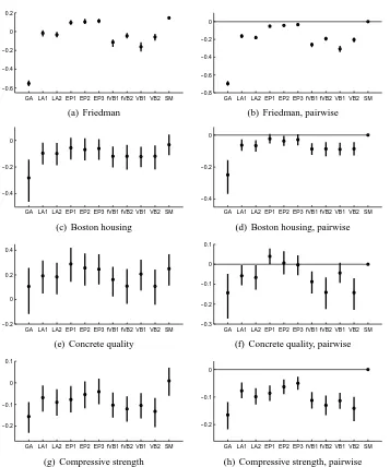
5.1 Simple Regression Examples
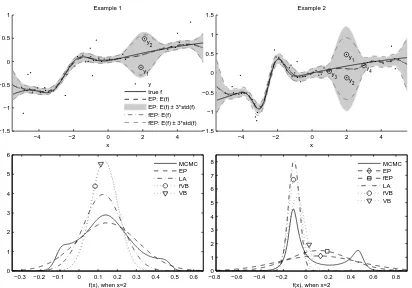
Figure 1 shows two one-dimensional regression problems in which standard EP may run into
prob-lems. In example 1 (the left subfigures), there are two outliers y1 and y2 providing conflicting
information in a region with no regular observations (1<x<3). In this example the posterior
mass of the length-scale is concentrated to sufficiently large value so that the GP prior is stiff and
keeps the marginal posterior p(f|
D
)(shown in the lower left panel) and the conditional posteriorp(f|
D
,θˆ,νˆ,σˆ2)at the MAP estimate unimodal. Both sequential and parallel EP converge with theMAP estimate for the hyperparameters.
The corresponding predictive distribution is visualized in the upper left panel of Figure 1
show-ing a considerable increase in the posterior uncertainty when 1<x<3. The lower left panel shows
comparison of the predictive distribution of f(x)at x=2 obtained with the different
approxima-tions described in Section 3. The hyperparameters are estimated separately for each method. The
smooth MCMC estimate of the predictive density of the latent value f∗= f(x∗)at input location x∗
is calculated by integrating analytically over f for each posterior draw of the residual variances V
and averaging the resulting Gaussian distributions q(f∗|x∗,V,θ). The MCMC estimate (with
inte-gration over the hyperparameters) is unimodal but shows small side bumps when the latent function
value is close to the observations y1 and y2. The standard EP estimate covers well the posterior
uncertainty on the latent value but both the Laplace method and fVB underestimate it. At the other input locations where the uncertainty is small, all methods give very similar estimates.
Even though EP remains stable in example 1 with the MAP estimates of the hyperparameters, it
is not stable with all hyperparameter values. Ifνandσ2were sufficiently small, so that the likelihood
p(yi|fi)was narrow as a function of fi, and the length-scale was small inducing small correlations
between inputs far apart, there would be significant posterior uncertainty about the unknown f(x)
when 1<x<3 and the true conditional posterior would be multimodal. Due to the small prior
covariances of the observations y1and y2with the other data points y3, ...,yn, the cavity distributions
q−1(f1)and q−2(f2)would differ strongly from the approximative marginal posterior distributions
q(f1)and q(f2). This difference would lead to a very small (or even negative) cavity precisionsτ−1
andτ−2during the EP iterations which causes stability problems as will be illustrated in section 5.2.
The second one-dimensional regression example, visualized in the upper right panel of Figure 1, is otherwise similar with example 1 except that the nonlinearity of the true function is much stronger
when−5<x<0, and the observations y1and y2are closer in the input space. The stronger
nonlin-earity requires a much smaller length-scale for a good data fit and the outliers y1and y2provide more
conflicting information (and stronger multimodality) due to the larger prior covariance. The lower
−4 −2 0 2 4 −1.5 −1 −0.5 0 0.5 1 Example 1 x y 1 y 2 y true f EP: E(f) EP: E(f) ± 3*std(f) fEP: E(f) fEP: E(f) ± 3*std(f)
−0.3 −0.2 −0.1 0 0.1 0.2 0.3 0.4 0.5 0.6
0 1 2 3 4 5 6
f(x), when x=2
MCMC EP LA fVB VB
−4 −2 0 2 4
−1.5 −1 −0.5 0 0.5 1 1.5 Example 2 x y 1 y 2 y 3 y 4
−0.8 −0.6 −0.4 −0.2 0 0.2 0.4 0.6 0.8
0 1 2 3 4 5 6 7 8
f(x), when x=2
MCMC EP fEP LA fVB VB
Figure 1: The upper row: Two one-dimensional regression examples, where standard EP may fail to converge with certain hyperparameter values, unless damped sufficiently. The EP
ap-proximations obtained by both the regular updatesη=1 (EP) and the fractional updates
η=0.5 (fEP) are visualized. The lower row: Comparison of the approximative
predic-tive distributions of the latent value f(x)at x=2. With MCMC all the hyperparameters
are sampled and for all the other approximations (except fVB in example 2, see the text for explanation) the hyperparameters are fixed to the corresponding MAP estimates. No-tice that the MCMC estimate of the predictive distribution is unimodal in example 1 and multimodal in example 2. With smaller lengthscale values the conditional posterior
p(f|
D
,θ,ν,σ2)can be multimodal also in example 1.The MCMC estimate has two separate modes near the observations y1 and y2. The Laplace and
fVB approximations are sharply localized at the mode near y1but the standard EP approximation
(EP1) is very wide trying to preserve the uncertainty about the both modes. Contrary to example
1, also the conditional posterior q(f|
D
,θ,ν,σ)is two-modal if the hyperparameters are set to theirMAP-estimates.
5.2 EP Updates with the Student-t Sites
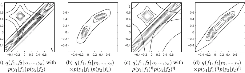
Next we discuss the problems with the standard EP updates with the help of example 1. Figure
2 illustrates a two-dimensional tilted distribution of the latent values f1 and f2 related to the
f2
f1
−0.4 −0.2 0 0.2 0.4 0.6 −0.4
−0.2 0 0.2 0.4 0.6
(a) q(f1,f2|y3, ...,yn)with
p(y1|f1)p(y2|f2)
−0.4 −0.2 0 0.2 0.4 0.6 −0.4
−0.2 0 0.2 0.4 0.6
(b) q(f1,f2|y3, ...,yn)
×p(y1|f1)p(y2|f2)
f2
−0.4 −0.2 0 0.2 0.4 0.6 −0.4
−0.2 0 0.2 0.4 0.6
(c) q(f1,f2|y3, ...,yn)with
p(y1|f1)ηp(y2|f2)η
−0.4 −0.2 0 0.2 0.4 0.6 −0.4
−0.2 0 0.2 0.4 0.6
(d) q(f1,f2|y3, ...,yn)
×p(y1|f1)ηp(y2|f2)η
Figure 2: An illustration of a two-dimensional tilted distribution related to the two problematic
data points y1 and y2 in example 1. Compared to the MAP value used in Figure 1,
shorter lengthscale (0.9) is selected so that the true conditional posterior is multimodal.
Panel (a) visualizes the joint likelihood p(y1|f1)p(y2|f2) together with the generalized
2-dimensional cavity distribution q(f1,f2|y3, ...,yn)obtained by one round of undamped
sequential EP updates on sites ˜ti(fi), for i=3, ...,n. Panel (b) visualizes the corresponding
two-dimensional tilted distribution ˆpi(f1,f2)∝q(f1,f2|y3, ...,yn)p(y1|f1)p(y2|f2).
Pan-els (c) and (d) show the same with only a fractionη=0.5 of the likelihood terms included
in the tilted distribution, which corresponds to fractional EP updates on these sites.
quite strong prior correlation between f1 and f2. Suppose that all other sites have already been
updated once with undamped sequential EP starting from a zero initialization (˜τi=0 and ˜νi=0 for
i=1, ...,n). Panel (a) visualizes a generalized 2-dimensional cavity distribution q(f1,f2|y3, . . . ,yn) together with the joint likelihood p(y1,y2|f1,f2) =p(y2|f2)p(y2|f2), and panel (b) shows the
con-tours of the resulting two dimensional tilted distribution which has two separate modes. If the site
˜t1(f1)is updated next in the sequential manner with no damping, ˜τ1will get a large positive value
and the approximation q(f1,f2)fits tightly around the mode near the observation y1. After this, when
the site ˜t2(f2)is updated, it gets a large negative precision, ˜τ2<0, since the approximation needs
to be expanded towards the observation y2. It follows that, the marginal precision of f1 is updated
to a smaller value than ˜τ1. Therefore, during the second sweep the cavity precisionτ−1=σ−12−τ˜1
becomes negative, and site 1 can no longer be updated. If the EP updates were done in parallel,
both the cavity and the site precisions would be positive after the first posterior update, but q(f1,f2)
would be tightly centered between the modes. After a couple of parallel loops over all the sites, one of the problematic sites gets a too small negative precision because the approximation needs to be expanded to cover all the marginal uncertainty in the tilted distributions which leads to a negative cavity precision for the other site.
Skipping updates on the sites with negative cavity variances can keep the algorithm
numeri-cally stable (see, for example, Minka and Lafferty, 2002). Also increasing damping reduces∆τ˜iso
that the negative cavity precisions are less likely to emerge. However, these modifications are not enough to ensure convergence. After a few EP iterations, the marginal posterior distribution of a
problematic site, for instance q(f1), is centered between the observations (see, for example, Figure
1). At the same time, the respective cavity distribution, q−1(f1), is centered near the other
problem-atic observation, y2. Combining such cavity distribution with the likelihood term, p(y1|f1), gives a
are sufficiently large (corresponding to a tight posterior approximation), the variance of the tilted
distribution will be larger than that of the marginal posterior and thus the site precision, ˜τ1will be
decreased. The same happens for the other site. The site precisions are decreased for a few itera-tions after which the posterior marginals are so wide that the variances of the tilted distribuitera-tions are smaller than the posterior marginal variances. At this point the site precisions start again to increase gradually. This leads to oscillation between small and large site precisions as illustrated in Figure 3.
With a smaller δ the oscillations are slower and with a sufficiently small δ the amplitude of
the oscillations may gradually decrease leading to convergence, as in the panel (b) of Figure 3. However, the convergence is not guaranteed since the conditions of the inner-loop maximization in (10) are not guaranteed to be fulfilled in sequential or parallel EP. For example, a sequential EP update can be considered as a one inner-loop step where only one site is updated, followed by an
outer-loop step which updates all the marginal posteriors as qsi(fi) =q(fi). Since the update of one
site does not maximize the inner-loop objective, the conditions used to form the upper bound of the convex part in (10) are not met (Opper and Winther, 2005). Therefore, the outer-loop objective is not guaranteed to decrease and the new approximate marginal posteriors may be worse than in the previous iteration.
Example 2 is more difficult in the sense that convergence requires damping at least withδ=0.5.
With sequential EP the convergence depends also on the update order of the sites andδ<0.3 is
needed for convergence with all permutations. Furthermore, if the double-loop approach of Section 4 is considered, the best step size, that minimizes the inner-loop objective in the current search direction, can change (and also increase) considerably between subsequent inner-loop iterations which makes the continuous step-size adjustments very useful.
Also fractional updates improve the stability of EP. Figures 2(c)–(d) illustrate the same
approx-imate tilted distribution as Figures 2(a)–(b) but now only a fractionη=0.5 of the likelihood terms
are included. This corresponds to the first round fractional updates on these sites with zero
initial-ization. Because of the flattened likelihood p(y1|f1)ηp(y2|f2)ηthe 2-dimensional tilted distribution
is still two-modal but less sharply peaked compared to standard EP on the left. It follows that also the one-dimensional tilted distributions have smaller variances and the consecutive fractional
up-dates (12) of the sites 1 and 2 do not widen the marginal variancesσ21andσ22as much. This helps to
keep the cavity precisions positive by increasing the approximate marginal posterior precisions and
reducing the possible negative increments on the site precisions ˜τ1and ˜τ2. This is possible because
the different divergence measure allows for a more localized approximation at 1<x<3. In
addi-tion, the property that a fraction(1−η)of the site precisions is left in the cavity distributions helps
to keep the cavity precisions positive during the algorithm. Figure 1 shows a comparison of standard
(EP) and fractional EP (fEP,η=0.5) with the MAP estimates of the hyperparameters. In example
1 both methods produce very similar predictive distribution because the posterior is unimodal. In example 2 (the lower right panel) fractional EP gives a much smaller predictive uncertainty
esti-mate when x=2 than standard EP which in turn puts more false posterior mass in the tails when
compared to MCMC.
The practical guidelines presented in Section 4 bring additional stability in the above described problematic situations. Modification 1 helps to avoid immediate problems from a too large step size by ensuring that each parallel EP update increases the inner-loop objective defined by (10).
Modification 2 reduces the step sizeδ so that the cavity variances, defined as τ−i =τsi−τ˜i with
fixed λs={νsi,τsi}, will remain positive during the inner-loop updates. Modification 3 reduces
4 6 8 10
(a) Sequential, δ=0.8
−log Z EP 0 20 40 60 Site precisions 4 6 8 10
(b) Sequential, δ=0.5
0 20 40 60 y 3 y 4 y
1 and y2
4 6 8 10
(c) Parallel, δ=0.5
0 20 40 60 10 20 30 (d) Double−loop −log Z EP
0 20 40 60 80 100
0 20 40 60 Site precisions Iterations 4 6 8 10
(e) 5 parallel + Double−loop
0 20 40 60 80 100
0 20 40 60 4 6 8 10
(f) Parallel, η=0.5
0 20 40 60 80 100
0 20 40 60
Figure 3: A convergence comparison between sequential and parallel EP as well as the double-loop algorithm in example 2 (the right panel in Figure 1). For each method both the
objective−log ZEPand the site precisions ˜τirelated to data points y1, ...,y4(see Figure 1)
are shown. See Section 5.3 for explanation.
the moments of ˆpi(fi)and q(fi)are consistent for fixedλsbefore updating qsi(fi). For example, a
poor choice ofδmay require many iterations for achieving inner-loop consistency in the examples
1 or 2, and a too largeδcan easily lead to a decrease of the inner-loop objective function or even
negative cavity precisions for the sites 1 or 2. Finally, if an unsuccessful update is made due to an
unsuitableδ, modification 4 enables automatic determination of a better step size by making use of
the concavity of the inner-loop maximization as well as the tilted and marginal moments evaluated
at the previous steps with the sameλs.
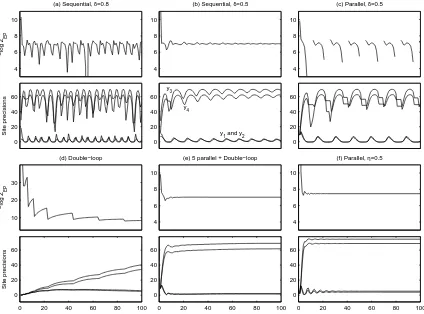
5.3 Convergence Comparisons
Figure 3 illustrates the convergence properties of the different EP algorithms using the data from
example 2. The hyperparameters were set to: ν=2, σ=0.1, σse=3 and lk =0.88. Panel (a)
shows the negative marginal likelihood approximation during the first 100 sweeps with sequential
the observations y1, ...,y4marked in the upper right panel of Figure 1. With this damping level the
site parameters keep oscillating with no convergence and there are also certain parameter values between iterations 50-60 where the marginal likelihood is not defined because of negative cavity
precisions (the updates for such sites are skipped until the next iteration). Whenever ˜τ1 and ˜τ2
become very small they also inflict large decrease in the site precisions of the nearby sites 3 and 4. These fluctuations affect other sites the more the larger their prior correlations are (defined by the GP prior) with the sites 1 and 2. Panel (b) shows the same graphs with larger amount of damping
δ=0.5. Now the oscillations gradually decrease as more iterations are done but convergence is
still very slow. Panel (c) shows the corresponding data with parallel EP and the same amount of damping. The algorithm does not converge and the oscillations are much larger compared to sequential EP. Also the marginal likelihood is not defined at many iterations because of negative cavity precisions.
Panel (d) in Figure 3 illustrates the convergence of the double-loop algorithm with no parallel initialization. There are no oscillations present because the increase of the objective (10) is verified at every iteration and sufficient inner-loop optimality is obtained before proceeding with the outer-loop minimization. However, compared to sequential or parallel EP, the convergence is very slow and it takes over 100 iterations to get the site parameters to the level that sequential EP attains with only a couple of iterations. Panel (e) shows that much faster convergence can be obtained by initializing with 5 parallel iterations and then switching to the double-loop algorithm. There is still some slow drift visible in the site parameters after 20 iterations but changes in the marginal likelihood estimate are very small. Small changes in the site parameters indicate inconsistencies in the moment matching conditions (7) and consequently also the gradient of the marginal likelihood
estimate may be slightly inaccurate if the implicit derivatives of log ZEP with respect to λ− and
λs are assumed zero in the gradient evaluations (Opper and Winther, 2005). Panel (f) shows that
parallel EP converges without damping if fractional updates withη=0.5 are applied. Because of
the different divergence measure the posterior approximation is more localized (see Figure 1) and also the cavity distributions are closer to the respective marginal distributions. It follows that the
site precisions related to y1and y2are larger and no damping is required to keep the updates stable.
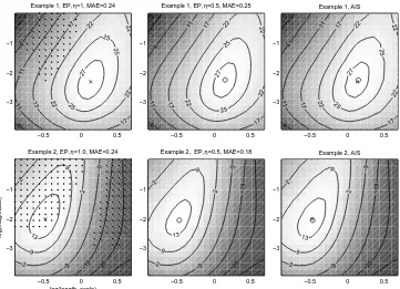
5.4 The Marginal Likelihood Approximation
Figure 4 shows contours of the approximate log marginal likelihood with respect to log(lk) and
log(σ2
se) in the examples of Figure 1. The contours in the first column are obtained by applying
first sequential EP withδ=0.8 and using the double-loop algorithm if it does not converge. The
hyperparameter values for which the sequential algorithm does not converge are marked with black
dots and the maximum marginal likelihood estimate of the hyperparameters is marked with (×).
The second column shows the corresponding results obtained with fractional EP (η=0.5) and
the corresponding hyperparameter estimates are marked with (◦). For comparison, log marginal
likelihood estimates determined with the annealed importance sampling (AIS) (Neal, 2001) are shown in the third column.
In the both examples there is an area of problematic EP updates with smaller length-scales which
corresponds to the previously discussed ambiguity about the unknown function near data points y1
and y2in Figure 1. There is also a second area of problematic updates at larger length-scale values
in example 2. With larger length-scales the model is too stiff and it is unable to explain large