Multiple-Instance Learning from Distributions
Gary Doran [email protected]
Soumya Ray [email protected]
Department of Electrical Engineering and Computer Science Case Western Reserve University
10900 Euclid Ave, Glennan 320 Cleveland, OH 44106, USA
Editor:Luc De Raedt
Abstract
We propose a new theoretical framework for analyzing the multiple-instance learning (MIL) setting. In MIL, training examples are provided to a learning algorithm in the form of la-beled sets, or “bags,” of instances. Applications of MIL include 3-D quantitative structure– activity relationship prediction for drug discovery and content-based image retrieval for web search. The goal of an algorithm is to learn a function that correctly labels new bags or a function that correctly labels new instances. We propose that bags should be treated as latent distributions from which samples are observed. We show that it is possible to learn accurate instance- and bag-labeling functions in this setting as well as functions that correctly rank bags or instances under weak assumptions. Additionally, our theoretical results suggest that it is possible to learn to rank efficiently using traditional, well-studied “supervised” learning approaches. We perform an extensive empirical evaluation that sup-ports the theoretical predictions entailed by the new framework. The proposed theoretical framework leads to a better understanding of the relationship between the MI and standard supervised learning settings, and it provides new methods for learning from MI data that are more accurate, more efficient, and have better understood theoretical properties than existing MI-specific algorithms.
Keywords: multiple-instance learning, learning theory, ranking, classification
1. Introduction
image given pixel color values. Again, using such an approach, it is not clear how one might identify which object in or region of the image was of interest to a user.
For such problems, the multiple-instance (MI) setting offers a richer representation for structure objects as sets, or “bags,” of feature vectors, each of which is called an “instance” (Dietterich et al., 1997). In the text categorization example above, a document is a bag of passages or paragraphs, which are the instances. For CBIR, an image is a bag of segments or objects. The MI setting further assumes that labels exist at both the level of instances and bags, where a bag’s label is the logical conjunction of Boolean instance labels. That is, a bag is positive ifat least one instance in the bag is positive and negative ifall of the instances in the bag are negative. This logical relationship corresponds to the fact that a document or an image is of the class of interest if and only if at least one of the passages or objects it contains is of the class of interest.
In the standard supervised setting, there is typically only one target concept of interest. For MI learning, one might be interested in learning either a bag or an instance concept from MI data. For example, in the 3-Dimensional Quantitative Structure–Activity Relationship (3D-QSAR) domain, the goal is to learn to predict whether a molecule will bind to a given target receptor (Dietterich et al., 1997). Because a molecule has flexible bonds, it exists in multiple shapes, or conformations, in solution. Thus, mapping this problem into the MI setting, conformations are instances and molecules are bags. A bag-labeling function can be used to predict whether a given molecule will bind to a target receptor. On the other hand, aninstance-labeling function can be used to predict which specific conformations will bind to a receptor, providing useful, difficult-to-measure information about the receptor’s physical structure.
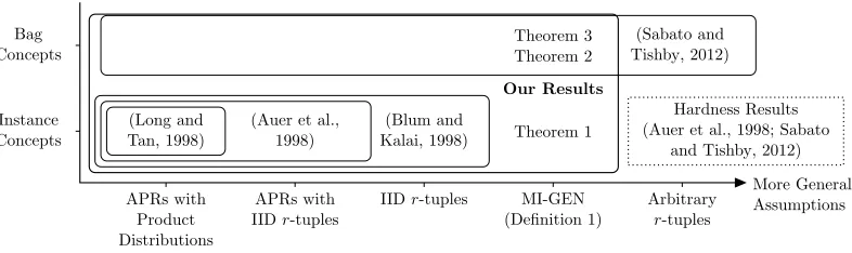
Despite the importance of these two learning tasks, only the bag-labeling task has re-ceived much attention in recent prior work characterizing the learnability of MI concepts (Sabato and Tishby, 2012). When learnability of instance concepts has been addressed, it has been under the strict, unrealistic assumption that instances across all bags are independent and identically distributed (IID) samples from the same underlying distri-bution (Blum and Kalai, 1998). However, as far as we know, the result of Blum and Kalai (1998) has remained the only positive result on instance concept learnability in the MI setting for over a decade. In this paper, we describe newpositive results for both instance-and bag-concept learnability. Our contributions are summarized as follows:
1. We describe a new generative model for MI data and show that it subsumes some previously proposed generative models for MI learning (MIL).
2. We provide novel results for learning accurate bag-level concepts from MI data.
3. We describe the first positive instance concept learnability results since those of Blum and Kalai (1998).1
4. We prove the first results, to our knowledge, that formally describe the ability to rank both instances and bags in the MI setting.
5. We empirically evaluate a surprising implication of our theoretical results: that stan-dard supervised approaches can effectively rank both instances and bags in the MI
setting. Our evaluation uses 55 data sets from a wide variety of domains, and sup-ports both our theoretical results as well as the assumptions made by our generative model.
2. Bags as Distributions
In this section, we describe a generative model for MI data in which bags are viewed as distributions over instances rather than as sets of instances. We show that the proposed generative model actually encompasses previous, standard models of MI learning in which bags are sets or tuples. The choice of framing a problem within a particular theoretical model has significant practical consequences for designing or selecting an algorithm to solve the problem. This section provides a theoretical framework in which the MI classification problem can be analyzed. The model allows us to derive positive instance- and bag-concept learnability results for the MI setting as described in Section 3. Furthermore, as Section 4 shows, the generative model leads to a surprising yet testable hypothesis that standard supervised algorithms can learn from MI data. This hypothesis is evaluated experimentally, supporting the assumptions made by the model.
2.1 The Generative Model
At the heart of this work is the claim that bags are best viewed as distributions rather than as finite sets of instances. Below, we formally define what we mean by this statement. But first, the example domain of drug activity prediction provides an intuitive justification for this claim. As described in Section 1, in the drug activity prediction domain, the goal is to predict the ability of molecules to activate, or bind to, a receptor. To cast the problem as binary classification, we select some threshold so that each molecule’s activity level either corresponds to an “active” or “inactive” label. In this case, we can think of each molecule (bag) as being drawn from a distribution DB over molecules. Ignoring for the moment
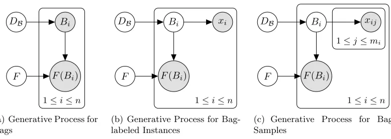
that each molecule has numerous conformations, this molecule either activates the receptor or not, so in nature the labeling function is defined at the level of bags. Prior models represent each molecule as a set or multiset of conformations, so they implicitly assume that each molecule exists in only a finite number of conformations. In reality, a molecule can transform continuously from conformation to conformation, producing an infinite set of conformations. In particular, each molecule exists in a state of dynamic equilibrium in which the amount of time it spends in each conformation is distributed according to Gibbs free energy such that low-energy conformations are preferred. Hence, the molecule (bag) corresponds to a distribution over instances. Constructing a bag from low-energy conformations, the common procedure for constructing bags in the drug activity domain, can be thought of as sampling instances from this distribution. Note that each molecule will have a unique distribution over conformations; thus, prior generative models for MIL that assume all instances are drawn from the same distribution are not applicable (Blum and Kalai, 1998). In Section 2.5, we describe how this view of the MI generative process can be applied to other problem domains.
Bi
F(Bi)
DB
F
1≤i≤n
(a) Generative Process for Bags
xi
Bi
F(Bi)
DB
F
1≤i≤n
(b) Generative Process for Bag-labeled Instances
xij
Bi
F(Bi)
DB
F
1≤j≤mi
1≤i≤n
(c) Generative Process for Bag Samples
Figure 1: A comparison of the generative processes for bags, individual bag-labeled in-stances, and bag samples.
function, in the MI setting there is also aninstance-labeling function with the standard MI assumption relating the bag- and instance-labeling functions. We describe theinstance dis-tribution that is consistent with the generative process, which will be useful for discussing instance concept learnability. In addition to these essential components, we introduce two additional weak assumptions that make efficient learning in this setting possible.
Bags as Distributions. To formalize the intuition above, suppose we have an instance spaceX. Typically, the space of bags is some subset ofX∗, the set of all finite subsets ofX. However, here, we let the space of bags be B =P(X), the set of probability distributions on the input space. Hence, each bag B ∈ B is a probability distribution over instances, denoted P(x |B).
Bag Distribution. We propose that, at the level of bags, the MI generative process is similar to that for supervised learning. In particular, bags are sampled from some fixed distributionDB, which is a distribution over instance distributions (DB ∈P(P(X))). From
this distributionDB, we sample some set of bags{Bi}ni=1, as illustrated by the plate model
in Figure 1(a).
Bag-Labeling Function. As in supervised learning, we assume that there exists some labeling function F : B → {0,1} that labels bags. Thus, a supervised data set
{(Bi, F(Bi))}ni=1 could be produced by sampling bags IID fromDB and applying the
label-ing functionF.
Instance-Labeling Function. In the MI setting, we assume that in addition to the bag-labeling function F, there also exists an instance-labeling function f : X → {0,1}. A key component of the MI setting is not only the existence of both bag and instance labeling functions, but the relationship between the two as well. Traditionally, the MI assumption is stated with respect to particular sets of instances so that a bag labelF(Bi) is
the logicalOR(for boolean labels), or maximum (for numerical labels), of its instances’ labels: F(Bi) = maxjf(xij). However, in the proposed generative model, bags are distributions
The MI Assumption. We state the relationship between F and f at the level of the generative model. Accordingly, a bag is negative (F(B) = 0) if and only if probability of sampling a positive instance within the bag is zero: Px∼B[f(x) = 1] = 0. In measure
theoretic terms, instances sampled within negative bags are almost surely negative, which implies that positive instances are almost surely sampled only within positive bags. This condition corresponds to the standard MI assumption that negative bags contain only neg-ative instances.
Instance Distribution. In order to talk about the learnability of f, we must define some instance distribution with respect to which we will measure risk. An instance dis-tribution naturally arises from our generative model if we first sample a bag B randomly from DB, then sample an instance x randomly from the distribution corresponding to B.
The instance distributionDX resulting from this two-level sampling procedure is effectively
the distribution that marginalizes out the individual bag distributions. That is, given a probability distribution PB over bags corresponding toDB, we can define a distribution PX
corresponding toDX as
PX(x) =
Z
B
P(x |B) dPB(B). (1)
Given that “x” is used to denote instances and “B” is used to denote bags, we subsequently drop subscripts from P when the sample space can be inferred from context. As we discuss in Section 3.4, the ability to marginalize out bag-specific distributions in our model plays a vital role in proving the learnability of instance- and bag-labeling functions. Given a bag distribution, the existence of such an instance distribution is guaranteed under relatively weak assumptions on the instance spaceX(Diestel and Uhl, 1977). Furthermore, note that while we can view instances in our generative model as being sampled IID from DX, this
does not require the assumption that instances are IID across all bag distributions, as in prior generative models for MIL (Blum and Kalai, 1998). We discuss this point in detail in Section 3.6.
Additional Assumptions. As is the case in the standard MI framework, in our generative model, only bag labels are observed. Suppose we sample individual instances as illustrated in Figure 1(b) where we first sample a bag, record its label, and then sample an instance from the bag-specific distribution P(x |B) and assign the bag label to the instance. Then the resulting bag-labeled instances{(xi1, F(Bi))}ni=1 are distributed according toDX,
and will appear in positive bags some of the time and negative bags the remaining fraction of the time. Therefore, each instance will have some probabilityc(x) ∈[0,1] of appearing with a positive label, which can be formally expressed as a probabilistic concept (p-concept) like the kind described by Kearns and Schapire (1994):
c(x),P [F(B) = 1|x]. (2)
That is, the probability of observing a positive label for instancex is the conditional prob-ability that the bag B in the two-level sampling procedure was positive, given that x was observed withinB. This conditional probability can be derived from the joint distribution over instances and bag labels corresponding to the generative process in Figure 1(b).
It follows from the previously-stated relationship between F and f that for any positive instance x+,c(x+) = 1, since each positive instance is observed almost surely (with
make the following weak assumption: there exists some γ >0 such that for every negative instance x−, c(x−) ≤ 1−γ. Intuitively, this corresponds to the assumption that every
negative instance is observed with some nonzero probability in a negative bag.
To see why negative instances must appear in negative bags in order to learn a concept, consider trying to learn the instance concept “spoon” in the CBIR domain, as described in Section 1. To learn this concept, you are given a set of images containing spoons, and a set of images not containing spoons. However, suppose that in every image containing a spoon, there is also a fork nearby. Furthermore, forks never appear alone in images without spoons. In this unfortunate scenario, you have no means of determining which of the fork or spoon is the positive instance given only image-level labels. However, if there is a guarantee that eventually you will see a negative image containing a fork but not a spoon, you will be able to learn that the fork is not the positive instance. We discuss learnability further in Section 3 and Section 4.
Finally, for learning bag-level concepts, we show in Section 3.2 that we require one additional assumption that there is some minimum fraction π of positive instances in each positive bag. That is, for every positive bag B+, P [f(x) = 1|B+] ≥ π. Without this
assumption, there might be positive bags that only contain negative instances. However, this would make them indistinguishable during bag labeling from negative bags, which by definition only contain negative instances. Interestingly, this assumption is not required if we are only interested in learning an instance-level concept.
Now, we can formally define MI-GEN, the set of generative processes for MI data con-sistent with the assumptions described above,
Definition 1 (MI-GEN) Given anyγ ∈(0,1]andπ∈[0,1],MI-GEN(γ, π)is the set of all tuples (DX, DB, f, F), each consisting of an instance distribution DX (with corresponding
P(x)), bag distribution DB (with corresponding P(B)), instance-labeling function f, and
bag-labeling functionF, that satisfy the conditions:
1. P(x) =R
BP(x |B) d P(B)
2. ∀x :f(x) = 1 =⇒ P [F(B) = 0|x] = 0
3. ∀x :f(x) = 0 =⇒ P [F(B) = 0|x]≥γ
4. ∀B :F(B) = 1 =⇒ P [f(x) = 1|B]≥π.
For simplicity, we will write MI-GEN(γ) for the case when π = 0, which corresponds to the weakest Condition 4. That is, for any fixed γ, MI-GEN(γ) ⊇MI-GEN(γ, π) for every π≥0. Such notation will be used when discussing instance-concept learnability, which does not require the π > 0 assumption. That is, instance-concept learning under our model is naturally tolerant to “bag label noise” of the form where positive bags contain only negative instances.
Finally, note that for any γ ∈(0,1], π∈[0,1], MI-GEN(γ, π)⊇MI-GEN(1,1). That is, γ =π = 1 corresponds to the strongest constraints on the generative process. Even in this case, foranyDX andf, there existDB andF such that (DX, DB, f, F)∈MI-GEN(1,1). In
particular, given a point mass δx centered onx, we can define DB so that PB(δx) = PX(x)
−1 0 1
X
1−θ θ
(a) P(x|Bθ)
0 π 1 θ Pneg
1−Pneg
1−π
(b) DB, P(Bθ)
−1 0 1
X
1−pneg pneg
(c) DX, P(x)
−1 0 1
X
1
1−γ
(d) c(x)
Figure 2: An example generative process for MI data. Each bag distribution (a) is parame-terized byθ, and the distribution over bags (b) corresponds to a distribution over values ofθ. The resulting distribution over instance (c) is derived in Equation 4 and Equation 5. The probability of instances appearing in positive bags (d) is derived in Equation 6 and Equation 7.
expressed in our generative model. That is, sampling from our generative process in that case is indistinguishable from sampling directly fromDX with labels assigned according to
f. Below, we discuss the relationship between our generative model and other proposed models for MI learning.
2.2 An Example of the Generative Process
As a concrete example, suppose the instance space is the closed real-valued interval X = [−1,1] and each bag Bθ is a distribution parameterized by a single real-valued parameter
θ ∈ [0,1]. As illustrated in Figure 2(a), the bag distribution P(x |Bθ) assigns (1−θ) of
the probability mass uniformly to the interval [−1,0), and θ of the mass uniformly to the interval [0,1]. Each value ofθcorresponds to a different bag, which is a different distribution over instances.
In this example, a distribution over bags is essentially a distribution over the bag pa-rameterθ. Such a distribution is illustrated in Figure 2(b), and assignsPneg of the mass to
the set {0}and the remaining 1−Pneg portion of the mass uniformly to the interval [π,1].
The probability of sampling a bag, P(Bθ), corresponds to the probability of sampling the
corresponding value ofθ. Similarly, a bag-labeling function F can be defined in terms ofθ as follows:
F(Bθ) =
(
0 ifθ= 0
1 ifθ >0. (3)
Thus, for this example, Pneg = P [F(Bθ) = 0].
For the sake of the example, we choose the instance-labeling function to be
f(x) = (
0 ifx <0 1 ifx ≥0.
This choice is consistent with the bag-labeling function defined in Equation 3, sinceF(Bθ) =
If we marginalize out the bag distribution, we obtain the single instance distribution in Figure 2(c). Analytically, for anyx− ∈[−1,0), we have
P(x−) =
Z 1 0
P(x−|Bθ) P(Bθ) dθ
= 1·Pneg+
Z 1
π
(1−θ)1−Pneg 1−π dθ =Pneg+12(1−Pneg)(1−π),pneg.
(4)
Similarly, for x+∈[0,1],
P(x+) =
Z 1
0
P(x+|Bθ) P(Bθ) dθ
= 0·Pneg+
Z 1
π
θ1−Pneg 1−π dθ = 12(1−Pneg)(1 +π) = 1−pneg.
(5)
Since probability density functions exist for this example, we can analytically compute c(x) given the following expression:
c(x) = P [F(B) = 1|x] = R
B+P(x|B) d P(B)
P(x) ,
whereB+={B:F(B) = 1}. As described, for positive instances x+ ∈[0,1], we have
c(x+) =
R1
π P(x+|Bθ) P(Bθ) dθ 1
2(1−Pneg)(1 +π)
= 1, (6)
since positive instances always appear in positive bags. On the other hand, for negative instances,
c(x−) =
R1
π P(x−|Bθ) P(Bθ) dθ
Pneg+12(1−Pneg)(1−π)
=
1
2(1−Pneg)(1−π)
Pneg+12(1−Pneg)(1−π) ,
1−γ.
(7)
The resulting values ofc(x) are shown in Figure 2(d). Note that for this generative process, except for the trivial case in which Pneg = 0, 1−γ = c(x−) < 1, so γ > 0. Thus, the
assumption that negative instances appear in negative bags is automatically satisfied for the example in Figure 2. By construction, this example also satisfies theπ >0 assumption since there is zero probability of sampling a bag with θ ∈ (0, π) mass over positive bags. Hence, this example is an element of MI-GEN.
2.3 The Empirical Bag-Labeling Function
DB Bi xij
F(Bi)
F f(xij) f
1≤j≤mi
b
F {xij}
1≤i≤n
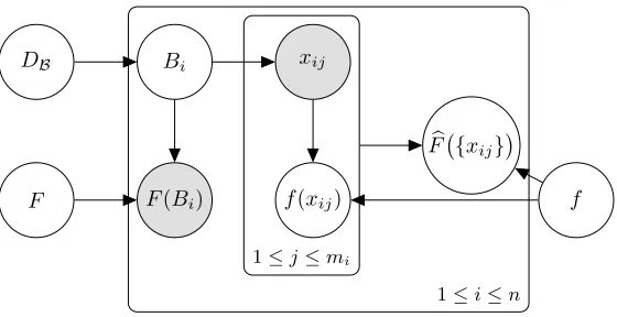
Figure 3: An illustration of the instance-, bag-, and empirical bag-labeling functions in MI-GEN.
However, in the standard MI setting, bag labels are typically viewed as being derived from instance labels. That is, if a bag is a set, then it is positive if it contains at least one positive instance, and negative otherwise.
Unlike the plate model in Figure 1(a), we do not typically observe bags directly in the MI setting. In the typical case, we only have access to samples Xi = {xij}mj=1i , each
drawn independently according to the distribution corresponding to each bag Bi so that
n
{xij}mj=1i , F(Bi)
on
i=1 is the observed MI data set, as shown in Figure 1(c). Each bag
can be a different size, but we will useml≤mi ≤mu to denote the lower and upper bounds
on bag sizes, respectively.
If we think of “bags” (in the sense of the standard generative model) of instances{xij}mj=1i
as empirical samples drawn from the underlying bag distributions Bi in our model, then it
is possible that samples from positive bags do not contain any positive instances. Hence, such “bags” would be negative in the sense of the standard model. To more harmoniously account for the standard notion of bag labels within our model, we introduce the empirical bag-labeling function, Fb:X∗→ {0,1}:
b
F(Xi) = max
j f(xij), (8)
whereXi={xij}mj=1i is any finite set of instances.
We can think of Fb as the bag labels that would be assigned by an oracle that had perfect information about the instance-labeling function f, but only an empirical sample from each bag. An illustration of the empirical bag-labeling function is shown in Figure 3. Figure 3 is a version of Figure 1(c) that shows the contributions of the instance-labeling and empirical bag-labeling functions. For every instancexij in an empirical bag sample,f
assigns the labelf(xij) to xij. On the other hand,Fb is a function of the entire bag sample Xi={xij}mj=1i as well as the instance-labeling function f, as specified in Equation 8.
Figure 4: An example from the CBIR domain when a positive image does not contain a positive instance (the notebook, annotated in blue) after segmentation.
F and Fb on positive bags if only negative instances are sampled within a positive bag. We return to characterizing the discrepancy betweenF andFb in Section 3.2.
The discrepancy between F and Fb is essentially bag-label noise that naturally results from our generative model. Previous generative models do not account for this potential source of label noise, despite its presence in some domains. For example, in the drug activity prediction domain, even if it is known that a molecule activates a receptor, a sample of conformations from this molecule might not contain the particular positive conformation that causes activation. Likewise, for the CBIR domain, extracting a set of objects from images is often performed using segmentation achieved through local optimization (Andrews et al., 2003; Carson et al., 2002). Therefore, it is possible that no single instance in a bag generated from a positive image will correspond to the positive instance. Figure 4 shows an example from the SIVAL data set when, due to lighting conditions, the positive “notebook” instance in the image is grouped with the table during segmentation (Settles et al., 2008). This kind of “noise” is naturally captured by our generative model as the discrepancy betweenFb and F.
2.4 Relationship to Prior Models
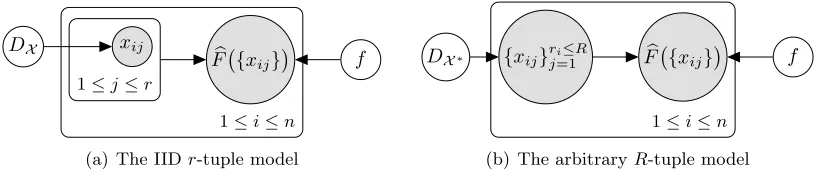
The most general model in which instance learnability results have been previously shown is the “IIDr-tuple” model (Blum and Kalai, 1998). The model, illustrated in Figure 5(a), assumes that each bag is generated by randomly samplingrinstances in every bag from the same underlying instance distribution, DX. However, this is an unrealistic assumption for
To show that our model is more general than the IID r-tuple model, we now describe how to simulate this model within our model. First, we define each bag to be a probability distribution parameterized by anr-tuple of instancesB(x1,...,xr). This distribution will be a
weighted sum of point masses over each of therinstances: P(x |B(x1,...,xr)) = 1 r
Pr
i=1δxi(x).
Then, for any distributionDX over instances (with P(x)) and instance-labeling functionf,
we let the distribution over bags DB be defined as P(B(x1,...,xr)) ,
Qr
i=1P(xi), which is
the probability that the corresponding r-tuple would have been sampled from DXr, and the bag-labeling function F to be F(B(x1,...,xr)) = max1≤i≤rf(xi). Let pneg = P [f(x) = 0],
then we claim that the (DX, DB, f, F) described above is in MI-GEN pr−1neg,1r
.
First, we need to show that DB as defined satisfies Condition 1 of Definition 1:
P(x)=? Z
B
P(x |B) d P(B)
= Z
B
1 r
r
X
i=1
δxi(x) d P(B(x1,...,xr))
= 1 r
r
X
i=1
Z
X· · ·
Z
X
δxi(x) d P(xr)· · · d P(x1)
= 1 r
r
X
i=1
Y
j6=i
Z
X
d P(xj)
Z
X
δxi(x) d P(xi)
= 1 r
r
X
i=1
1r−1
P(x) = P(x).
So sampling instances under our two-step generative process is equivalent to sampling ac-cording to the original instance distribution.
Condition 2 of Definition 1 is trivially satisfied, since by the definition of F, positive instances never appear in negative bags. To show that Condition 3 holds, we must compute the probability that negative instances appear in a negative bag. Using the definition of conditional probability, this is,
P [F(B) = 0|x] = R
B−P(x |B) d P(B)
Using the fact that in a negative bag B(x1,...,xr), all instances must be negative, we can compute the numerator for a negative instance as
Z
B−
P(x |B) d P(B) = Z B− 1 r r X i=1
δxi(x) d P(B(x1,...,xr))
= 1 r r X i=1 Z X− · · · Z X−
δxi(x) d P(xr)· · · d P(x1)
= 1 r r X i=1 Y j6=i Z X−
d P(xj)
Z X−
δxi(x) d P(xi)
= 1 r r X i=1
pr−1neg
P(x) =pr−1neg P(x).
Thus, P [F(B) = 0|x] = prneg−1P(x) P(x) = p
r−1
neg. Since this probability is the same across all
negative instances, this means thatγ =pr−1neg. This quantity is positive as long aspneg>0.
Otherwise, all instances are positive, so the γ >0 assumption is vacuously satisfied. Finally, to show that Condition 4 of Definition 1 is satisfied, we see that for a positive bag,Bi,
P [f(x) = 1|B] = Z
X
f(x) 1 r
r
X
i=1
δxi(x)
! dx = 1 r r X i=1
f(xi)≥
1 r =π,
(9)
since at least one instance in the bag is such that f(x) = 1. Therefore, the IID r-tuple model is a special case of our model in which γ and π are positive, and determined by the fraction of negative instances and bag size r.
Another generative model, used to show the learnability of bag-level concepts (Sabato and Tishby, 2012), allows arbitrary distributions over r-tuples. The model further relaxes ther-tuple model by allowing bag sizes to vary from 1 toR, some maximum bag size. The model is illustrated in Figure 5(b), whereDX∗ denotes the distribution over tuples of size at mostR. However, this model is also restrictive for many problem domains like drug activity prediction, since it enforces that bag sizes are finite and bounded, whereas molecules can exist in infinitely many conformations.
We can also represent the generative model of Sabato and Tishby (2012) in a similar way as for the IIDr-tuple model. We simplify the space of bags to be atomic distributions over r ≤R tuples, and allow an arbitrary distributionDB over bags rather than requiring that
P(B(x1,...,xr)) =
Qr
i=1P(xi). Now,DX is not fixed, so we can define it in terms of Condition 1
of MI-GEN so that that condition is automatically satisfied. The bag-labeling function F is still defined in terms of the arbitrary instance-labeling function f, so Condition 2 is still trivially satisfied. Furthermore, by similar reasoning as in Equation 9, π = 1
R
xij
1≤j≤r
b
F {xij}
DX
f
1≤i≤n
(a) The IIDr-tuple model
{xij}rji≤=1R Fb {xij}
DX∗ f
1≤i≤n
(b) The arbitraryR-tuple model
Figure 5: Previous generative models for MI data.
concept learnability with MI-GEN 0,R1
, we require MI-GEN γ,R1⊂MI-GEN 0,R1 for instance concept learnability.
Babenko et al. (2011) propose treating bags in the MI setting as manifolds in the instance space X. While this allows describing a bag with an infinite number of instances, it assigns an equal “weight” to every instance. However, for a domain like drug activity prediction, a molecule is more likely to exist in certain conformations than in others. The varying weight of instances is naturally handled in our setting, but we do not treat bags as manifolds over instances, so our results may not apply to the generative process in which bags are manifolds.
Some prior work proposes additional generative models for MIL, some of which model bags as distributions over instances. For example, some work uses Gaussian distributions (Maron and Lozano-P´erez, 1998; Xu, 2003) or mixture models (Foulds and Smyth, 2011) to represent distributions over instances, while other work uses more complex graphical (Yang et al., 2009; Adel et al., 2013; Kandemir and Hamprecht, 2014) or hierarchical Bayesian (Kuck and de Freitas, 2005) models. However, our work differs from these prior investiga-tions in two important ways. First, we focus on the theoretical properties of our generative model, whereas prior work has only empirically explored the performance of algorithms tailored to specific generative models. Secondly, while prior generative models require that bags or instances are sampled from specific, parametric probability distributions, our gen-erative model does not require such assumptions. Thus, the theoretical results presented below apply to more general scenarios than the models previously explored.
2.5 Applicability to Problem Domains
At the beginning of this section, we motivated MI-GEN using the 3D-QSAR domain. In this section, we elaborate on how bags can naturally be viewed as distributions in various other problem domains and which labeling tasks illustrated in Figure 3 are of interest in each domain. Of course, as described in Section 2.4, standard generative models are special cases of MI-GEN, so previous applications of MIL for which it is most natural to think of bags as finite sets of instances can still be incorporated in this model.
2.5.1 Drug Activity Prediction
instance-labeling function f. Knowing whether an individual conformation binds to a receptor provides information about the structure of the receptor’s binding site, which is practically difficult to measure directly. Hence, learning both instance- and bag-labeling functions are important in the 3D-QSAR domain.
2.5.2 Text Categorization
While it is popular to represent documents as a flat “bag of words” using a single feature vector comprised of word frequencies (Salton and McGill, 1983), prior work has acknowl-edged the benefits of representing document-specific structure. In particular, latent Dirich-let allocation (LDA) models each document as a mixture of distributions over words (Blei et al., 2003). Of course, LDA can also applied to a coarser-grained representation in which documents are distributions overn-grams or paragraphs, which are like individual instances in the MI setting (Blei et al., 2003). Other work attempts to infer the level of granularity in a document in addition to modeling the distributions over the discovered “segments” (Du et al., 2013). Hence, treating documents as distributions is already a natural and popular representation for text. On the other hand, LDA treats each document distribution as tak-ing a specific parametric form, whereas our results and analysis do not make any parametric assumptions about bag-level distributions.
As for 3D-QSAR, both document-level and instance-level categorization is important in the text categorization domain. For example, if certain types of documents like survey articles discuss various subjects, then it might be important to determine not just that the document as a whole discusses a particular subject, but also which specific passage or paragraph discusses the subject.
2.5.3 Content-Based Image Retrieval
Applying our generative framework to the CBIR task requires viewing images as distribu-tions over objects such that the objects in each image are a sample from the corresponding distribution. As with LDA for the text categorization domain, analogous probabilistic mod-els have been proposed for categorizing natural scenes (Fei-Fei and Perona, 2005). Thus, while treating images as distributions is not unprecedented, our analysis is novel in that it discuses learnability under such a model without assuming that image distributions take a specific parametric form.
Furthermore, as for the other domains discussed, the bag-labeling function F is not the only latent variable of interest in CBIR. In additional to labeling new images, a CBIR system might be interested in determining the location of the object of interest within an image, which requires learning the instance-labeling functionf.
3. Learning Accurate Concepts from MI Data
Table 1: A summary of the learnability results in Section 3 and Section 4.
Accuracy AUC
Instance f Theorem 1 Theorem 4
Bag Fb Theorem 2 Theorem 5 F Theorem 3 Theorem 6
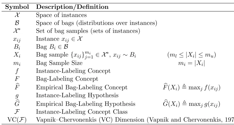
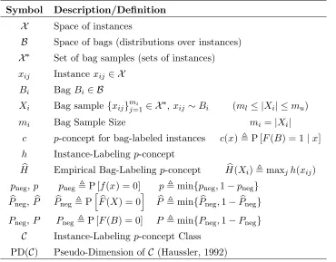
Table 2: Legend of the basic notation used in Section 3.
Symbol Description/Definition
X Space of instances
B Space of bags (distributions over instances)
X∗ Set of bag samples (sets of instances) xij Instancexij ∈ X
Bi BagBi ∈ B
Xi Bag sample{xij}mj=1i ∈ X ∗,x
ij ∼Bi (ml≤ |Xi| ≤mu)
mi Bag Sample Size mi=|Xi|
f Instance-Labeling Concept F Bag-Labeling Concept
b
F Empirical Bag-Labeling Concept F(Xb i),maxjf(xij) g Instance-Labeling Hypothesis
b
G Empirical Bag-Labeling Hypothesis G(Xb i),maxjg(xij)
F Instance-Labeling Concept Class
VC(F) Vapnik–Chervonenkis (VC) Dimension (Vapnik and Chervonenkis, 1971)
to rank instances and bags from MI data. Table 1 summarizes the theoretical contributions made in this and the following sections, which demonstrate the learnability of the instance conceptf, empirical bag-labeling function F, and bag-labeling functionb F with respect to both accuracy and ranking as measured by area under ROC (AUC). The results in this section and the following section use a model of the instance labeling functionf to derive models for the bag-labeling functionsFb and F.
Defining the ability of an algorithm to learn a good approximation of a target concept requires some metric by which the quality of the approximation is to be measured. Tra-ditionally, the quality of a classifier is measured in terms of expected 0–1 loss. We begin by investigating the ability of algorithms to learn accurate concepts from MI data in this sense. While there is only one learning task in the supervised setting, there are now both instance- and bag-concept learning tasks in the MI setting, which we explore separately in the following sections. Table 2 shows the notation used for the concepts in this section.
3.1 Learning Accurate Instance Concepts
described in Section 2 differs from that for supervised learning, we must restate what it means to “PAC” learn an accurate instance concept under this model.
In the supervised setting, the learnability of some fixed concept class F is discussed without making any assumptions about the distribution over instances. The definition of MI-GEN in Definition 1 similarly allows any instance distribution, with which many bag distributions are consistent in the sense of Condition 1. To ensure that the target concept f is a member of the concept classF, we must further restrict the set of models allowed by the generative process as follows:
Definition 2 (MI-GENF) For any γ ∈(0,1] andπ ∈[0,1]:
MI-GENF(γ, π),
(DX, DB, f, F)∈MI-GEN(γ, π) :f ∈ F .
Now, we can formally define PAC learnability for the MI setting:
Definition 3 (Instance MI PAC-learning) We say that an algorithmAMI PAC-learns instance concept class F from MI data when for any (DX, DB, f, F) ∈ MI-GENF(γ) with
γ > 0, and I, δ > 0, A requires O poly(γ1,I1,1δ)
bag-labeled instances sampled indepen-dently from the MI generative process in Figure 1(b) to produce an instance hypothesis g with risk Rf(g)< I with probability at least 1−δ over samples.2
Note that because our generative model allows us to discuss the marginalized instance distribution DX, the risk Rf(g) = Ex∼DX
1[f(x) 6= g(x)]
is measured with respect to this distribution as in the supervised setting. Now we show that instance concepts are MI PAC-learnable in the sense of Definition 3:
Theorem 1 An instance concept class F with VC dimensionVC(F)is Instance MI PAC-learnable using OIγ1 VC(F) log 1
Iγ + log 1 δ
examples.
Proof By Condition 1 in Definition 1, we can treat bag-labeled instances as being drawn from the underlying instance distributionDX. Instances are observed with some label noise
with respect to true labels given by f. Since positive instances never appear in negative bags (by Condition 2 of Definition 1), noise on instances is one-sided. If every negative instance appears in negative bags at least some γ fraction of the time (by Condition 3), then the maximum one-sided noise rate isη= 1−γ. Since γ >0,η <1, which is required for learnability. Under our generative assumptions, the noise is “semi-random” in that noise rate might vary across instances, but is bounded byη <1. Thus, learning an instance concept is equivalent to learning from data with one-sided label noise in this sense.
The result of Simon (2012) shows that in the presence of one-sided, semi-random noise, when a concept class F has a VC dimension of VC(F), F is PAC-learnable from OI(1−η)1 VC(F) log 1
I(1−η) + log1δ
examples using a “minimum one-sided disagree-ment” strategy. This strategy entails choosing a classifier that minimizes the number of dis-agreements on positively-labeled examples while perfectly classifying all negatively-labeled examples. This strategy also works in the special case that all instances and bags are posi-tive (η= 0, orγ = 1, since there are no negative instances). Substituting 1−γ forηin the
bound of Simon (2012) yields the bound in terms ofγ.
We note that Theorem 1 allows for “noisy” positive bags without positive instances (π = 0), since the additional bag-level noise is essentially absorbed intoη.
3.2 Learning Accurate Bag Concepts
As for instance concept learnability, we must formally define what we mean to learn accurate bag concepts in the MI setting. As described in Section 2, there are two bag-labeling functions we might be interested in learning. In our generative model, we assume that the MI relationship between bag and instance labels holds at the level of the generative process. That is, bags are directly assigned labels by a bag concept F. On the other hand, given a set of instances sampled from a bag, we might be interested in learning the more traditional bag-labeling concept in the MI setting, Fb(Xi) = maxjf(xij), which we have called the empirical bag-labeling function (Equation 8). We will first analyze learnability with respect to the empirical bag-labeling function and then extend this result to the true bag-labeling function.
We can define the risk of a bag-labeling concept Gb with respect to the underlying empirical bag-labeling conceptFb as follows:
RFb(G) = Eb
1[Fb(X)6=G(X)]b
= Z
B
Z
X∗1[ b
F(X)6=G(X)] d P(Xb |B) d P(B),
(10)
where P(X | B) is the probability of sampling the set of instances X from bag B. Since we assume that instances are sampled IID according to B, P(X | B) = Q
x∈XP(x | B).
Given a formal definition of the risk of an empirical bag-labeling function, we can define learnability with respect to this function below:
Definition 4 (Empirical Bag MI PAC-learning) We say that an algorithmAMI PAC-learns empirical bag-labeling functions derived from instance concept class F when for any (DX, DB, f, F) ∈ MI-GENF(γ) with γ > 0, and B, δ > 0, A requires O poly(1γ,B1 ,1δ)
bag-labeled instances sampled independently from the MI generative process in Figure 1(b) to produce an empirical bag-labeling function Gb with risk R
b
F(G)b < B with probability at least 1−δ over samples.
To show empirical bag concept learnability under our generative model, we will show that by learning an accurate enough instance conceptg, the resulting empirical bag-labeling concept given byG(Xb i) = maxjg(xij) will have low risk with respect toFb. Thus, we start with a bound onR
b
F(G) in terms ofb Rf(g).
Lemma 1 Let Rf(g) be the risk of an instance labeling concept g, and RFb(G)b be the risk of the empirical bag-labeling function G(Xb i) = maxjg(xij). Then if bag sample sizes are bounded by mu (∀i:|Xi| ≤mu), RFb(G)b ≤muRf(g).
Proof See Appendix A.
Theorem 2 Empirical bag-labeling functions derived from instance concept class F with VC dimension VC(F) are PAC-learnable from MI data using
O
mu Bγ
VC(F) logmu Bγ+ log
1 δ
examples.
Proof The general strategy is to learn an approximation gforf ∈ F using minimum one-sided disagreement as mentioned in the proof of Theorem 1 and then to derive an empirical bag-labeling functionGb fromg.
For a desired bound B on RFb(G), by usingb I = mB
u in Theorem 1, this ensures that
the resulting instance classifier is such that Rf(g) < mBu with high probability. Combined
with the result in Lemma 1, this implies that R b
F(G)b ≤ muRf(g) < mu
B mu
= B, so
RFb(G)b < B as desired. SubstitutingI= mB
u into the bound in Theorem 1 gives the bound
as stated in Theorem 2.
Again, Theorem 2 allows for noisy positive bags without positive instances (π = 0). Fur-thermore, in the special case when every bag sample is a singleton X={x}, then mu = 1
and Fb({x}) =f(x). Thus, the instance concept learnability result in Theorem 1 is really just a special case of learning an empirical bag-labeling function with bags of size 1 as in Theorem 2.
Next, we turn our attention to learning the underlying bag-labeling functionF. We will still use the instance-labeling function g to derive this bag-labeling function. It is possible to consider learningF without the use of an instance conceptg, as we discuss in Section 3.3. During both training and testing, we are only given access to a sample Xi from each bag
Bi with which we can estimate F(Bi). Therefore, we will again learn an empirical bag
labeling function G(Xb i). However, now we will assess the quality of Gb with respect to the underlying bag-labeling function F as follows:
RF(G) = Eb
1[F(B)6=G(X)]b
= Z
B
Z
X∗1[F(B)6= b
G(X)] d P(X|B) d P(B). (11)
The definition of bag concept learnability then takes the same form as that in Definition 4 with the risk as given in Equation 11. As we will show in Lemma 2, we now also require the further assumption that π, minimum fraction of positive instances in positive bags, is nonzero.
Definition 5 (Bag MI PAC-learning) We say that an algorithmAMI PAC-learns bag-labeling functions derived from instance concept class F when for any (DX, DB, f, F) ∈
MI-GENF(γ, π) with γ, π > 0, and B, δ > 0, algorithm A requires O poly(1γ,π1,B1 ,1δ)
bag-labeled instances sampled independently from the MI generative process in Figure 1(b) to produce an empirical bag-labeling function Gb with risk RF(G)b < B with probability at least 1−δ over samples.
an empirical bag-labeling conceptG. Since Theorem 2 shows that we can a learn a conceptb
b
Gthat accurately modelsFb, what remains to be shown is thatFbis an accurate model ofF under some additional conditions. First, we prove the following lemma, which decomposes the riskRF(G) into the discrepancy betweenb Gb andFb, and the discrepancy betweenFb and F.
Lemma 2 For any empirical bag-labeling concept Gb,
RF(G)b ≤R b
F(G) +b RF(Fb).
Proof See Appendix A.
Now, we derive a bound on the discrepancy between the empirical bag-labeling function
b
F and the underlying bag-labeling function F. Since this discrepancy arises when we do not sample a positive instance within a positive bag, the bound depends on the minimum bag sample size and the minimum fractionπ of positive instances in every positive bag.
Lemma 3 Suppose bag samples are of size at least ml (∀i : ml ≤ |Xi|), then RF(Fb) ≤ (1−π)ml.
Proof See Appendix A.
Finally, we can now show the following learnability result with respect to the underlying bag-labeling function. However, note that in Lemma 3, the errorRF(Fb) decreases with the minimum bag sizeml. Thus, in order to achieve low error with respect toF, we must ensure
that bags in the test set are sufficiently large. Therefore, the following result is stated under the additional condition that the test bag sample sizes mi satisfy some constraints. Note
that these constraints arise naturally from the process that samples instances from bag distributions.
Theorem 3 Bag-labeling functions derived from instance concept class F with VC dimen-sion VC(F) are PAC-learnable from MI data using
O
1 2
Bγπ
VC(F) logBγπ1 + log1δ (12)
examples when test bag sample sizes are bounded by ml ≤m ≤mu and ml is large enough
such that ml≥ π1 logB2 .
Proof Intuitively, we can learn an instance-labeling function g according to Theorem 1 and then use the resulting empirical bag-labeling function G. By combining the previouslyb stated results, we can boundRF(G) asb
RF(G)b ≤R b
F(G) +b RF(Fb) (by Lemma 2)
≤muRf(g) +RF(Fb) (by Lemma 1)
In the case that π = 1, then the second term in the sum is zero. Otherwise, suppose the minimum bag size is such that
ml≥ π1logB2 ≥
logB2
log(1−π) = log1−π
B 2 ,
where the second inequality follows from the fact that π ≤ −log(1−π) for π ∈ (0,1). Therefore, since (1−π)<1, we have that
(1−π)ml ≤(1−π)log1−π B
2 = B 2 .
Furthermore, when learning the instance concept g, we can choose I to be such that
I = 2mBu. Since g will be such that Rf(g) < I with probability (1−δ), with the same
probability we have that
RF(G)b ≤muRf(g) + (1−π)ml
< mu
B 2mu
+B2 =B.
Substituting the expression for I in terms ofB into the bound in Theorem 1 gives the
sample complexity bound:
Omu Bγ
VC(F) log mu Bγ + log
1 δ
,
which is the same bound as stated in Theorem 2.
It is also possible to sub-sample large bags such that there is also a conservative upper bound on sample size mu = O
1 Bπ
, which is consistent with ml ≥ π1logB2 . Then, we
can derive an expression for learnability in terms ofπ. Substituting this bound into that of Theorem 2 gives the second sample complexity bound as stated in Equation 12.
3.3 Discussion
The results presented in Section 3.1 and Section 3.2 follow the same basic strategy. First, minimum one-sided disagreement is used to learn an accurate instance concept g in the presence of one-sided noise on bag-labeled instances. Then, for the bag-labeling task, in-stance labels are aggregated using an empirical bag-labeling functionGb to approximate the empirical bag-labeling function Fb or the underlying bag-labeling functionF. The idea of combining instance labels to produce a bag-labeling function is used by many existing MI algorithms.
More General Assumptions Instance
Concepts Bag Concepts
(Long and Tan, 1998)
APRs with Product Distributions
(Auer et al., 1998)
APRs with IIDr-tuples
(Blum and Kalai, 1998)
IIDr-tuples
Hardness Results (Auer et al., 1998; Sabato
and Tishby, 2012) Our Results
MI-GEN (Definition 1)
Theorem 3 Theorem 2
Theorem 1
(Sabato and Tishby, 2012)
Arbitrary
r-tuples
Figure 6: Relation to prior learnability results.
the other hand, the result in Theorem 2 suggests that it is harder to learn from larger bag sizes, since roughlyO(mulogmu) more examples are required to learn an accurate concept.
Essentially, the source of this incoherence in reasoning is the use of an instance-labeling conceptgto derive the bag-labeling conceptG. In the process of combining instance labelsb to label a bag, small errors in the instance labeling function g compound quickly. For example, g must label all instances in a negative bag correctly for Gb to label the bag correctly. As bag size increases, it becomes less likely that g will agree with f across all instances.
Therefore, despite our positive results suggesting that learning an accurate instance-labeling function is sufficient to learn an accurate bag-instance-labeling function, in practice, it is possible to imagine an alternative approach in which bag-labeling functions are learned directly by representing bags in a supervised fashion. Several practical approaches, such as bag-level kernels (G¨artner et al., 2002; Zhou et al., 2009) and embeddings (Chen et al., 2006; Foulds, 2008) do precisely this, and essentially turn the bag-label learning problem into a supervised learning problem. Further investigating the trade-offs between techniques that classify bags using instance classifiers and those that directly learn bag classifiers is an interesting direction for future work.
3.4 Relation to Prior Learnability Results
across instances. Hence, our results rely on the recent work of Simon (2012), which shows that it is possible to learn from instances corrupted with semi-random one-sided noise.
The bag learnability results in Section 3.2 show that an accurate bag concept can be learned by learning an accurate instance concept and deriving a bag concept by combining instance labels within a bag. Other recent work on bag concept learnability takes a different approach. The strategy of Sabato and Tishby (2012) is to directly learn empirical bag-labeling concepts using empirical risk minimization (ERM). That is, they suppose that an algorithm selects an instance-labeling function g ∈ F that minimizes RFb(G). Sinceb general sample complexity bounds exist for ERM in terms of capacity measures such as VC dimension of a hypothesis class (Blumer et al., 1989), Sabato and Tishby (2012) proceed by proving that the capacity of the function class nGb:G(Xb i) = maxjg(xij), g∈ F
o is bounded in terms of the capacity of F. In fact, the results of Sabato and Tishby (2012) apply to more general cases in which the combining function used to derive a bag-labeling function from an instance-labeling function is other than the max function. However, the results of Sabato and Tishby (2012) do not prove positive results about instance-labeling concepts.
As indicated in Figure 6, the results in Section 3.2 are not a strict generalization of those in Sabato and Tishby (2012), nor are those in Sabato and Tishby (2012) a generalization of those in Section 3.2. In particular, since MI-GEN treats bags as distributions, the results in Section 3.2 apply to cases not considered in Sabato and Tishby (2012), in which bags are assumed to have finite size. On the other hand, while our generative model can encapsulate aspects of the generative model in Sabato and Tishby (2012) (see Section 2.4), arbitrary distributions overr-tuples are not permitted. However, it may be that we are able to prove positive instance learnability results precisely because of this constraint on the generative process.
3.5 Relation to Prior Hardness Results
The positive learnability results in Section 3.1 and Section 3.2 do not contradict existing hardness results about learning in the MI setting. Essentially, most hardness results are shown under the scenarios that lie on the far right of Figure 6. For example, Sabato and Tishby (2012) observe that if only positive bags are generated, then learning the bag-labeling function is trivial, but no label information about instances is provided. In this case, learning instance labels is equivalent to learning in the unsupervised learning setting, for which no PAC-style guarantees can be made. However, the additional assumptions in MI-GEN preclude the case when only positive bags appear, since the negative instances would never appear in negative bags as required by Condition 3 in Definition 1.
Similarly, under the weak assumption in which arbitrary distributions over r-tuples are allowed, Auer et al. (1998) show that that efficiently PAC-learning MI instance concepts is impossible (unlessNP=RP3). While the results on instance and bag learnability stemming
from Theorem 1 show that a polynomial number of examples can be used to learn accurate concepts, they do not bound the computational complexity of learning from the examples. In particular, minimum one-sided disagreement is known to beNP-hard for certain concept classes and loss functions (Simon, 2012). Therefore, for some concept classes, instance and bag concepts are not efficiently PAC-learnable: learnable with a polynomial number of examples in polynomial time.
The apparent contradiction between our learnability results and the hardness results of Auer et al. (1998) is resolved by observing that MI-GEN precludes the scenario used to reduce learning disjunctive normal form (DNF) formulae to learning APRs from MI data. In the reduction used by Auer et al. (1998), each instance corresponds to a (variable assignment, clause) pair, and a bag is formed for each variable assignment by including a pair with that variable assignment for each clause. Bags are sampled uniformly over all variable assignments. Suppose a particular variable assignment v satisfies the first clause c1, but not the second clausec2. Then the instance (v, c1) is positive, but (v, c2) is negative.
However, (v, c2) only ever appears in bags along with (v, c1); that is, in positive bags. This
violates the condition that γ >0, or that negative instances appear with some probability in negative bags, so our results do not apply to this hard scenario.
Similarly, our generative model precludes scenarios used to show the hardness of learning hyperplane concepts for MI data (Kundakcioglu et al., 2010; Diochnos et al., 2012; Doran and Ray, 2013). It is unknown whether there is an algorithm to efficiently learn hyperplanes that minimize one-sided disagreement. However, even ERM under 0–1 loss isNP-hard for the concept class of hyperplanes (Ben-David et al., 2003), which are widely used in practice for supervised learning. Thus, while previous results have characterized the hardness of MI learning as resulting from arbitrary distributions across bags, our results suggest that the hardness arises from cases in whichγ = 0, or when negative instances only occur in negative bags.
3.6 Must Instances be Dependent Samples?
As observed in prior work, most real-world examples of MIL have bags that contain non-IID instances (Zhou et al., 2009). Thus, our assumption that bag samples Xi are drawn IID
according to their corresponding bag distributions Bi might seem unrealistic. However,
note that our generative modeldoes allow for dependencies between instances at the level of bag distributions, Bi. That is, although the samples Xi are drawn from bag
distribu-tions independently, we can use such independent samples to approximate the behavior of empirical bag-labeling functions on nonindependent samples.
The arbitrary R-tuple model, as illustrated in Figure 5(b), allows for arbitrary distri-butions over tuples of size at mostR, which can be used to represent any generative model in which there is a relationship between instances in bags (i.e., bags in which instances are non-IID). As described in Section 2.4, it is possible to represent this model within MI-GEN where each bag is an atomic distribution over the instances in the tuple and the distribution over bags corresponds to the original distribution over tuples. Given this representation, π = R1 in our model. In the traditional MI setting, we would directly observe theseR in-stances. Our generative model, on the other hand, assumes that we perform the equivalent of repeatedly sampling an instance from these R instances uniformly and independently at random. In this case, we have the following result:
Corollary 1 (MI PAC-learning from Dependent Instances) When distributions of instances in bags are defined by a set of R dependent instances sampled from a distri-bution over R tuples, bag-labeling functions derived from instance concept class F with VC dimension VC(F) are PAC-learnable from MI data using
OBγR log 1 B
VC(F) log R Bγ+ log
1 δ
examples with test bags of size m=lRlog 2 B
m
drawn independently with replacement from the R dependent instances.
Proof Following the same line of reasoning as in Theorem 3, we can derive the sample complexity bound
OBγm VC(F) logBγm + log1δ, (13)
when there are m instances per bag. Choosing m = lRlog 2 B
m
satisfies the conditions of that theorem, sinceπ= 1
R. Substitutingminto Equation 13 implies the sample complexity
as stated in the corollary.
Thus, even though the bag distribution is representable using only R dependent instances, when sampling independently, we must sample a factor of O
logB1 more instances to ensure that we can learn an accurate bag-labeling concept with high probability.
4. Learning to Rank from MI Data
Table 3: Legend of the basic notation used in Section 4.
Symbol Description/Definition
X Space of instances
B Space of bags (distributions over instances)
X∗ Set of bag samples (sets of instances) xij Instancexij ∈ X
Bi BagBi∈ B
Xi Bag sample{xij}mj=1i ∈ X ∗,x
ij ∼Bi (ml≤ |Xi| ≤mu)
mi Bag Sample Size mi=|Xi|
c p-concept for bag-labeled instances c(x),P [F(B) = 1|x] h Instance-Labelingp-concept
b
H Empirical Bag-Labelingp-concept H(Xb i),maxjh(xij)
pneg,p pneg,P [f(x) = 0] p,min{pneg,1−pneg}
b
Pneg,Pb Pbneg ,P h
b
F(X) = 0i Pb,min{Pbneg,1−Pbneg} Pneg,P Pneg,P [F(B) = 0] P ,min{Pneg,1−Pneg}
C Instance-Labelingp-concept Class PD(C) Pseudo-Dimension ofC (Haussler, 1992)
predict the activity of every molecule. Instead, a classifier can produce a ranked list in-dicating its confidence that each molecule is active. The set of active molecules with the highest predicted activity can then be investigated further by chemists. Unlike the prior work on learning accurate concepts from MI data as shown in Figure 6, there has been virtually no prior work on learning to rank in the MI setting. That is, although ranking algorithms have been developed for MIL (Bergeron et al., 2008), there is no formal analysis of the performance of such approaches. We provide such an analysis in this section.
4.1 Learning High-AUC Instance Concepts
Prior work has shown that the AUC is equivalent to the probability that a randomly selected positive example will be assigned a higher confidence than a randomly selected negative example (Hanley and McNeil, 1982). We can define a corresponding instance AUC error of a real-valued hypothesis h as 1−AUC, or the probability that a negative instance is assigned a higher confidence than a positive instance:
RAUCf (h) = Z
X
Z
X1
[h(x−)> h(x+)] d P(x+|f(x+) = 1) d P(x−|f(x−) = 0)
= R
X− R
X+1[h(x−)> h(x+)] d P(x+) d P(x−)
P [f(x) = 1] P [f(x) = 0]
= 1
(1−pneg)pneg
Z
X− Z
X+1
[h(x−)> h(x+)] d P(x+) d P(x−).
(14)
The first step follows from the definition of conditional probability, and we introducepneg=
P [f(x) = 0] for notational convenience (see Table 3 for a list of notation used in this section). By definition, this quantity is zero in the cases when either all instance are positive or all instances are negative.
Given the formal definition of AUC, we can begin to describe how it is possible to learn high-AUC instance concepts from MI data. Since a classifier’s confidence values are relevant for the AUC metric, we will consider the hypothesis class corresponding to a classifier to be ap-concept classC. Thep-concept model is a model for binary classification in which ap-conceptc:X →[0,1] represents the probability that an instanceXis observed with a positive label (Kearns and Schapire, 1994). For high-AUC instance learnability, we will show that it is sufficient to learn a p-concept h ∈ C that models the p-concept c(x) = P [F(B) = 1|x], the probability of observing instancex in a positive bag as defined in Equation 2.
To ensure that the target conceptcis also a member ofC, we must formally restrict the set of bag labeling functions and distributions that are permitted by the generative model as follows:
Definition 6 (MI-GENC) For any γ ∈(0,1] and π∈[0,1]:
MI-GENC(γ, π),
n
(DX, DB, f, F)∈MI-GEN(γ, π) : x 7→P [F(B) = 1|x]∈ C
o .
Learnability of a p-concept with high AUC is then defined with respect to p-concept classC:
Definition 7 (Instance MI AUC-PAC-learning) We say that an algorithmAMI AUC-PAC-learns instancep-concept classCfrom MI data when for any(DX, DB, f, F)∈MI-GENC(γ)
with γ >0, and I, δ >0, algorithm A requires O poly(1γ,I1,1δ)
bag-labeled instances sam-pled independently from the MI generative process in Figure 1(b) to produce an instance p-concept hypothesis h with risk RAUCf (h)< I with probability at least 1−δ over samples.
0 1−γ 1−γ
2 1
) (
c(x−) h(x−)
c(x+)
h(x+)
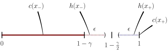
Figure 7: The intuition behind Theorem 4. A hypothesishthat closely approximatescwill correctly rank instances with high probability.
concepts using ERM. In particular, the strategy used in the following theorem is to learn a p-concept h that models the concept c defined in Equation 2 using standard ERM. The intuition is thatc already achieves perfect AUC; that is, RAUC
f (c) = 0. The reason is that
for any negative instance x− and positive instance x+, c(x−) ≤ 1−γ < 1 = c(x+), see
Figure 7 for an illustration. If we learn ap-concepth that closely approximatescto within some, then with high probability,h will also correctly rank instances.
Stating the learnability of a p-concept with ERM requires use of the pseudo-dimension of the concept class C, just as VC dimension can be used to characterize the capacity of a deterministic concept class. The pseudo-dimension is similar to the VC dimension, but uses a different notion of “shattering.” In particular, for a set of points with real-valued labels,{(xi, yi)}ni=1, ap-concept classC shatters the points if for any binary labeling of the
points {bi}, there exists some c∈ C such that c(xi) ≥yi ifbi = 1 andc(xi) < yi if bi = 0
(Haussler, 1992). The pseudo-dimension of C, denoted PD(C), is the size of the largest set such thatC shatters some set of that size.
Theorem 4 An instance p-concept class C with pseudo-dimension PD(C) is Instance MI AUC-PAC-learnable usingO(Iγp)1 4
PD(C) log 1
Iγp + log 1 δ
examples with standard ERM approaches, where p= min{pneg,1−pneg}.
Proof See Appendix A.
4.2 Learning High-AUC Bag Concepts
As for accuracy, we might be interested in learning either high-AUC instanceor bag concepts from MI data. Following a similar strategy as employed in Section 3.2 for learning accurate bag concepts, here we will consider two measures of bag-level performance of a bag concept
b
H derived from an instance concept h. The same combining function as in Section 3,
b
H(Xi) = maxjh(xij), is commonly used to derive real-valued bag-labeling functions in
prior work (Ray and Craven, 2005). Following the analysis in Section 3.2, we will measure performance ofHb with respect to bothFb, the empirical bag-labeling function, and laterF, the underlying bag-labeling function.
For the empirical bag-labeling function, Fb, the intuitive definition of AUC is the prob-ability that a bag-level hypothesisHb assigns a higher value to a bag sample given that it is labeled positive byFb (that is, containing at least one positive instance) than another bag sample labeled negative by Fb (containing no positive instances). Formally, we can define the corresponding AUC-based risk as follows:
RAUC b
F (H) =b
R B R B R X∗ − R X∗ +1 b
H(X−)>H(Xb +)
. . .
. . .d P(X+|B+) d P(X− |B−) d P(B+) d P(B−)
PhFb(X) = 1 i
PhFb(X) = 0 i = R B R B R
X∗− R
X∗+1
b
H(X−)>H(Xb +)
. . .
. . .d P(X+|B+) d P(X− |B−) d P(B+) d P(B−)
(1−Pbneg)Pbneg
.
(15)
Above,X∗−is the set of all negative bag samples, andX∗+the set of all positive bag samples.
The notationPbneg= Pr h
b
F(X) = 0iis used for convenience. Now, we can define learnability with respect to this metric:
Definition 8 (Empirical Bag MI AUC-PAC-learning) We say that an algorithm A
MI AUC-PAC-learns empirical bag-labeling functions derived from p-concept class C when for any (DX, DB, f, F) ∈ MI-GENC(γ) with γ > 0, and B, δ > 0, algorithm A requires
O poly(γ1,B1 ,1δ)
bag-labeled instances sampled independently from the MI generative
pro-cess in Figure 1(b) to produce an empirical bag-labeling functionHb with riskRAUC b
F (H)b < B
with probability at least 1−δ over samples.
We will now show learnability of empirical bag-labeling functions by reducing the prob-lem to learning an accurate model of the p-concept c. Hence, the approach of the proof follows that for learning accurate empirical bag-labeling functions.
Theorem 5 Empirical bag-labeling functions derived from p-concept class C with pseudo-dimension PD(C) are AUC-PAC-learnable from MI data using
O
m4 u
(BγPb)
4
PD(C) log mu
(BγPb)
+ log1δ
examples with standard ERM approaches, where
b
P ,min{Pneg,b 1−Pnegb } ≥min{Pneg,1−pneg},
Proof See Appendix A.
Note that Theorem 4 is a special case of Theorem 5 whenmu= 1. In this case Pbneg =pneg when samples all have size 1, so Pb=p and the sample complexity is the same.
Now, we can examine AUC-learnability with respect to the true bag-labeling function, F. To define AUC with respect to F, we measure the probability that a sample X+ is
labeled higher by Hb than X− is, given that X+ is sampled from a positive bag and X− is
sampled from a negative bag. Formally, the AUC risk of Hb with respect toF is
RAUCF (H) =b R
B− R
B+
R
X∗ R
X∗1
b
H(X−)>H(Xb +)
. . .
. . .d P(X+|B+) d P(X− |B−) d P(B+) d P(B−)
P [F(B) = 1] P [F(B) = 0]
= R
B− R
B+
R
X∗ R
X∗1
b
H(X−)>H(Xb +)
. . .
. . .d P(X+|B+) d P(X− |B−) d P(B+) d P(B−)
(1−Pneg)Pneg
.
(16)
The notationPneg= P [F(B) = 0] is used to denote the probability of sampling a negative
bag from the distribution over bags. We define the risk to be zero in the case that this probability is equal to either 0 or 1.
As for accuracy, the risk of an empirical bag-labeling function now depends on how representative a sample is of the underlying bag. Thus, in the definition of AUC-learnability with respect toF(Definition 9), we now again require an additional assumption that positive instances appear someπ >0 fraction of the time in positive bags.
Definition 9 (Bag MI AUC-PAC-learning) We say that an algorithm A MI AUC-PAC-learns bag-labeling functions derived from the p-concept class C when for any tuple (DX, DB, f, F) ∈MI-GENC(DX, f, γ, π) with γ, π >0, and B, δ >0, algorithm A requires
O poly(γ1,π1,B1,1δ)
bag-labeled instances sampled independently from the MI generative
pro-cess in Figure 1(b) to produce an empirical bag-labeling functionHb with riskRFAUC(H)b < B with probability at least 1−δ over samples.
Again, we will learn an instance p-concept h that models c, and then show that a suf-ficiently accuratep-concept can produce an empirical bag-labeling function Hb that models F with high AUC. To do this, we will show that the AUC error of Hb with respect to F, RFAUC(H), is bounded in terms of the AUC error ofb Hb with respect toFb,RAUC
b
F (H).b
Lemma 4 Suppose bag samples are of size at least ml (∀i:ml ≤ |Xi|), then RAUCF (H)b ≤
1 PnegR
AUC
b
F (H) + (1b −π) ml.
Proof See Appendix A.
Finally, given the bound in Lemma 4, we can derive a result on learning high-AUC bag concepts with respect to the underlying bag-labeling function F. As with the results in Theorem 3, we state the results conditioned on the fact that bag sizes mi respect some