Revisiting the Nystr{\"{o}m} Method for Improved Large-scale Machine Learning

(1)

Revisiting the Nystr¨

om Method for Improved Large-scale

Machine Learning

Alex Gittens [email protected]

Michael W. Mahoney [email protected]

International Computer Science Institute and Department of Statistics University of California, Berkeley

Berkeley, CA

Editor:Mehryar Mohri

Abstract

We reconsider randomized algorithms for the low-rank approximation of symmetric pos-itive semi-definite (SPSD) matrices such as Laplacian and kernel matrices that arise in data analysis and machine learning applications. Our main results consist of an empir-ical evaluation of the performance quality and running time of sampling and projection methods on a diverse suite of SPSD matrices. Our results highlight complementary as-pects of sampling versus projection methods; they characterize the effects of common data preprocessing steps on the performance of these algorithms; and they point to important differences between uniform sampling and nonuniform sampling methods based on leverage scores. In addition, our empirical results illustrate that existing theory is so weak that it does not provide even a qualitative guide to practice. Thus, we complement our empirical results with a suite of worst-case theoretical bounds for both random sampling and ran-dom projection methods. These bounds are qualitatively superior to existing bounds—e.g., improved additive-error bounds for spectral and Frobenius norm error and relative-error bounds for trace norm error—and they point to future directions to make these algorithms useful in even larger-scale machine learning applications.

Keywords: Nystr¨om approximation, low-rank approximation, kernel methods, random-ized algorithms, numerical linear algebra

1. Introduction

(2)

Our empirical results point to several directions that are not explained well by existing theory. (For example, that the results are much better than existing worst-case theory would suggest, and that sampling with respect to the statistical leverage scores leads to results that are complementary to those achieved by projection-based methods.) Thus, we complement our empirical results with a suite of worst-case theoretical bounds for both random sampling and random projection methods. These bounds are qualitatively superior to existing bounds—e.g., improved additive-error bounds for spectral and Frobenius norm error and relative-error bounds for trace norm error. By considering random sampling and random projection algorithms on an equal footing, we identify within our analysis deterministic structural properties of the input data and sampling/projection methods that are responsible for high-quality low-rank approximation.

In more detail, our main contributions are fourfold.

• First, we provide an empirical illustration of the complementary strengths and weak-nesses of data-independent random projection methods and data-dependent random sampling methods when applied to SPSD matrices. We do so for a diverse class of SPSD matrices drawn from machine learning and data analysis applications, and we consider reconstruction error with respect to the spectral, Frobenius, and trace norms. Depending on the parameter settings, the matrix norm of interest, the data set un-der consiun-deration, etc., one or the other method might be preferable. In addition, we illustrate how these empirical properties can often be understood in terms of the structural nonuniformities of the input data that are of independent interest.

• Second, we consider the running time of high-quality sampling and projection algo-rithms. For random sampling algorithms, the computational bottleneck is typically the exact or approximate computation of the importance sampling distribution with respect to which one samples; and for random projection methods, the computa-tional bottleneck is often the implementation of the random projection. By exploiting and extending recent work on “fast” random projections and related recent work on “fast” approximation of the statistical leverage scores, we illustrate that high-quality leverage-based random sampling and high-quality random projection algorithms have comparable running times. Although both are slower than simple (and in general much lower-quality) uniform sampling, both can be implemented more quickly than a na¨ıve computation of an orthogonal basis for the top part of the spectrum.

• Third, our main technical contribution is a set of deterministic structural results that hold for any “sketching matrix” applied to an SPSD matrix. We call these “determin-istic structural results” since there is no randomness involved in their statement or analysis and since they depend on structural properties of the input data matrix and the way the sketching matrix interacts with the input data. In particular, they high-light the importance of the statistical leverage scores, which have proven important in other applications of random sampling and random projection algorithms.

(3)

how high-quality random sampling algorithms and high-quality random projection algorithms can be treated from a unified perspective.

A novel aspect of our work is that we adopt a unified approach to these low-rank ap-proximation questions—unified in the sense that we consider both sampling and projection algorithms on an equal footing, and that we illustrate how the structural nonuniformities responsible for high-quality low-rank approximation in worst-case analysis also have im-portant empirical consequences in a diverse class of SPSD matrices. By identifying deter-ministic structural conditions responsible for high-quality low-rank approximation of SPSD matrices, we highlight complementary aspects of sampling and projection methods; and by illustrating the empirical consequences of structural nonuniformities, we provide theory that is a much closer guide to practice than has been provided by prior work. We note also that our deterministic structural results could be used to check, in ana posteriori manner, the quality of a sketching method for which one cannot establish ana priori bound.

Our analysis is timely for several reasons. First, in spite of the empirical successes of Nystr¨om-based and other randomized low-rank methods, existing theory for the Nystr¨om method is quite modest. For example, existing worst-case bounds such as those of Drineas and Mahoney (2005) are very weak, especially compared with existing bounds for least-squares regression and general low-rank matrix approximation problems (Drineas et al., 2008, 2010; Mahoney, 2011).1 Moreover, many other worst-case bounds make very strong assumptions about the coherence properties of the input data (Kumar et al., 2012; Gittens, 2012). Second, there have been conflicting views in the literature about the usefulness of uniform sampling versus nonuniform sampling based on the empirical statistical leverage scores of the data in realistic data analysis and machine learning applications. For example, some work has concluded that the statistical leverage scores of realistic data matrices are fairly uniform, meaning that the coherence is small and thus uniform sampling is appropri-ate (Williams and Seeger, 2001; Kumar et al., 2012); while other work has demonstrappropri-ated that leverage scores are often very nonuniform in ways that render uniform sampling inap-propriate and that can be essential to highlight properties of downstream interest (Paschou et al., 2007; Mahoney and Drineas, 2009). Third, in recent years several high-quality nu-merical implementations of randomized matrix algorithms for least-squares and low-rank approximation problems have been developed (Avron et al., 2010; Meng et al., 2014; Woolfe et al., 2008; Rokhlin et al., 2009; Martinsson et al., 2011). These have been developed from a “scientific computing” perspective, where condition numbers, spectral norms, etc. are of greater interest (Mahoney, 2012), and where relatively strong homogeneity assumptions can be made about the input data. In many “data analytics” applications, the questions one asks are very different, and the input data are much less well-structured. Thus, we expect that some of our results will help guide the development of algorithms and implementations that are more appropriate for large-scale analytics applications.

In the next section, Section 2, we start by presenting some notation, preliminaries, and related prior work. Then, in Section 3 we present our main empirical results; and in

(4)

Section 4 we present our main theoretical results. We conclude in Section 5 with a brief discussion of our results in a broader context.

2. Notation, Preliminaries, and Related Prior Work

In this section, we introduce the notation used throughout the paper, and we address several preliminary considerations, including reviewing related prior work.

2.1 Notation

Let A ∈_Rn×n _{be an arbitrary SPSD matrix with eigenvalue decomposition} _A ₌_UΣUT_, where we partition U andΣas

U= U1 U2 and Σ=

Σ1 Σ2

. (1)

Here,U1 hask columns and spans the top k-dimensional eigenspace ofA, and Σ1∈Rk×k is full-rank.2 We denote the eigenvalues of Awith λ1(A)≥. . .≥λn(A).

GivenA and a rank parameterk, the statistical leverage scores of Arelative to the best rank-k approximation to A equal the squared Euclidean norms of the rows of the n×k

matrixU1:

`j =k(U1)jk2. (2)

The leverage scores provide a more refined notion of the structural nonuniformities of A than does the notion of coherence, µ = n_kmax_i∈{1,...,n}`i, which equals (up to scale) the largest leverage score; and they have been used historically in regression diagnostics to identify particularly influential or outlying data points. Less obviously, the statistical lever-age scores play a crucial role in recent work on randomized matrix algorithms: they define the key structural nonuniformity that must be dealt with in order to obtain high-quality low-rank and least-squares approximation of general matrices via random sampling and random projection methods (Mahoney, 2011). Although Equation (2) defines them with respect to a particular basis, the statistical leverage scores equal the diagonal elements of the projection matrix onto the span of that basis, and thus they can be computed from any basis spanning the same space. Moreover, they can be approximated more quickly than the time required to compute that basis with a truncated SVD or a QR decomposition (Drineas et al., 2012).

We denote by S an arbitrary n×` “sketching” matrix that, when post-multiplying a matrix A, maps points from Rn to R`. We are most interested in the case where S is a random matrix that represents a random sampling process or a random projection process, but we do not impose this as a restriction unless explicitly stated. We let

Ω1 =UT₁S and Ω2 =UT₂S (3)

denote the projection ofS onto the top and bottom eigenspaces of A, respectively.

(5)

Recall that, by keeping just the top k singular vectors, the matrix Ak := U1Σ1UT1 is the best rank-kapproximation toA, when measured with respect to any unitarily-invariant matrix norm, e.g., the spectral, Frobenius, or trace norm. For a vector x∈ _Rn_{, let} _kxk

ξ, forξ= 1,2,∞,denote the 1-norm, the Euclidean norm, and the∞-norm, respectively, and let Diag(A) denote the vector consisting of the diagonal entries of the matrix A. Then, kAk₂ = kDiag(Σ)k∞ denotes the spectral norm of A; kAk_F = kDiag(Σ)k2 denotes the

Frobenius norm of A; and kAk_? =kDiag(Σ)k₁ denotes the trace norm (or nuclear norm) of A. Clearly,

kAk₂≤ kAk_F ≤ kAk_?≤√nkAk_F ≤nkAk₂.

We quantify the quality of our algorithms by the “additional error” (above and beyond that incurred by the best rank-k approximation to A). In the theory of algorithms, bounds of the form provided by (16) below are known asadditive-error bounds, the reason being that the additional error is an additive factor of the formtimes a size scale that is larger than the “base error” incurred by the best rank-k approximation. In this case, the goal is to minimize the “size scale” of the additional error. Bounds of this form are very different and in general weaker than when the additional error enters as a multiplicative factor, such as when the error bounds are of the form kA−Ak ≤˜ f(n, k, η)kA−Akk, where f(·) is some function and η represents other parameters of the problem. These latter bounds are of greatest interest when f = 1 +, for an error parameter , as in (18) and (19) below. Theserelative-error bounds, in which the size scale of the additional error equals that of the base error, provide amuch stronger notion of approximation than additive-error bounds.

2.2 Preliminaries

(6)

whether the data are sparse or dense, how the eigenvalue spectrum decays, the nonunifor-mity properties of eigenvectors,e.g., as quantified by the statistical leverage scores, whether one is interested in reconstructing the matrix or performing a downstream machine learning task, and so on.

The following sketching model subsumes both of these classes of methods.

• SPSD Sketching Model. Let A be an n×n positive semi-definite matrix, and let S be a matrix of size n×`, where `n. Take

C=AS and W=STAS.

Then CW†CT is a low-rank approximation to A with rank at most`.

We should note that the SPSD Sketching Model, formulated in this way, is not guaranteed to be numerically stable: ifW is ill-conditioned, then instabilities may arise in forming the productCW†CT. For simplicity in our presentation, we do not describe the generalizations of our results that could be obtained for the various algorithmic tweaks that have been considered to address this potential issue (Drineas et al., 2008; Mahoney and Drineas, 2009; Chiu and Demanet, 2013).

The choice of distribution for the sketching matrix S leads to different classes of low-rank approximations. For example, if S represents the process of column sampling, either uniformly or according to a nonuniform importance sampling distribution, then we refer to the resulting approximation as a Nystr¨om extension; if S consists of random linear combi-nations of most or all of the columns of A, then we refer to the resulting approximation as a projection-based SPSD approximation. In this paper, we focus on Nystr¨om extensions and projection-based SPSD approximations that fit the above SPSD Sketching Model. In particular, we do not consider adaptive schemes, which iteratively select columns to pro-gressively decrease the approximation error. While these methods often perform well in practice (Belabbas and Wolfe, 2009b,a; Farahat et al., 2011; Kumar et al., 2012), rigorous analyses of them are hard to come by—interested readers are referred to the discussion in (Farahat et al., 2011; Kumar et al., 2012).

2.3 The Power Method

One can obtain the optimal rank-kapproximation toA by forming an SPSD sketch where the sketching matrix S is an orthonormal basis for the range of Ak, because with such a choice,

CW†CT =AS(STAS)†STA=A(SSTASST)†A=A(PAkAPAk)

†_A₌_AA†

kA=Ak.

Of course, one cannot quickly obtain such a basis; this motivates considering sketching matrices Sq obtained using the power method: that is, taking Sq = AqS0 where q is a positive integer and S0 ∈Rn×` withl ≥k. Asq → ∞,assuming UT1S0 has full row-rank, the matrices Sq increasingly capture the dominant k-dimensional eigenspaces of A (see Golub and Van Loan, 1996, Chapter 8), so one can reasonably expect that the sketching matrixSq produces SPSD sketches ofA with lower additional error.

(7)

produce. Thus, the power method is most applicable whenAis such that one can compute the product AqS0 fast. We consider the empirical performance of sketches produced using the power method in Section 3, and we consider the theoretical performance in Section 4.

2.4 Related Prior Work

Motivated by large-scale data analysis and machine learning applications, recent theoretical and empirical work has focused on “sketching” methods such as random sampling and random projection algorithms. A large part of the recent body of this work on randomized matrix algorithms has been summarized in the recent monograph by Mahoney (2011) and the recent review article by Halko et al. (2011). Here, we note that, on the empirical side, both random projection methods (e.g., Bingham and Mannila, 2001; Fradkin and Madigan, 2003; Venkatasubramanian and Wang, 2011; Banerjee et al., 2012) and random sampling methods (e.g., Paschou et al., 2007; Mahoney and Drineas, 2009) have been used in applications for clustering and classification of general data matrices; and that some of this work has highlighted the importance of the statistical leverage scores that we use in this paper (Paschou et al., 2007; Mahoney and Drineas, 2009; Mahoney, 2011; Yip et al., 2014). In parallel, so-called Nyström-based methods have also been used in machine learning applications. Originally used by Williams and Seeger to solve regression and classification problems involving Gaussian processes when the SPSD matrixAis well-approximated by a low-rank matrix (Williams and Seeger, 2001; Williams et al., 2002), the Nyström extension has been used in a large body of subsequent work. For example, applications of the Nyström method to large-scale machine learning problems include the work of Talwalkar et al. (2008); Kumar et al. (2009a,c); Mackey et al. (2011b) and Zhang et al. (2008); Li et al. (2010); Zhang and Kwok (2010), and applications in statistics and signal processing include the work of Parker et al. (2005); Belabbas and Wolfe (2007a,b); Spendley and Wolfe (2008); Belabbas and Wolfe (2008, 2009b,a).

Much of this work has focused on new proposals for selecting columns (e.g., Zhang et al., 2008; Zhang and Kwok, 2009; Liu et al., 2010; Arcolano and Wolfe, 2010; Li et al., 2010) and/or coupling the method with downstream applications (e.g., Bach and Jordan, 2005; Cortes et al., 2010; Jin et al., 2013; Homrighausen and McDonald, 2011; Machart et al., 2011; Bach, 2013). The most detailed results are provided by Kumar et al. (2012) as well as the conference papers on which it is based (Kumar et al., 2009a,b,c). Interestingly, they observe that uniform sampling performs quite well, suggesting that in the data they considered the leverage scores are quite uniform, which also motivated the related works of Talwalkar and Rostamizadeh (2010); Mohri and Talwalkar (2011). This is in contrast with applications in genetics (Paschou et al., 2007), term-document analysis (Mahoney and Drineas, 2009), and astronomy (Yip et al., 2014), where the statistical leverage scores were seen to be very nonuniform in ways of interest to the downstream scientist; we return to this issue in Section 3.

On the theoretical side, much of the work has followed that of Drineas and Mahoney (2005), who provided the first rigorous bounds for the Nystr¨om extension of a general SPSD matrix. They show that when Ω(k−4lnδ−1) columns are sampled with an importance sampling distribution that is proportional to the square of the diagonal entries of A, then

kA−CW†CTk_ξ ≤ kA−Akkξ+

Xn

k=1(A) 2

(8)

holds with probability 1−δ, where ξ = 2, F represents the Frobenius or spectral norm. (Actually, they prove a stronger result of the form given in Equation (4), except with W† replaced withW†_k, whereWkrepresents the best rank-kapproximation toW(Drineas and Mahoney, 2005).) Subsequently, Kumar, Mohri, and Talwalkar show that if µkln(k/δ)) columns are sampled uniformly at random with replacement from an A that has exactly rankk, then one achieves exact recovery,i.e.,A=CW†CT, with high probability (Kumar et al., 2009a). Gittens (2012) extends this to the case whereA is only approximately low-rank. In particular, he shows that if ` = Ω(µklnk) columns are sampled uniformly at random (either with or without replacement), then

A−CW

† CT

2≤ kA−Akk2

1 +2n

`

(5)

with probability exceeding 1−δ and

A−CW

† CT

2 ≤ kA−Akk2+ 2

δ · kA−Akk? (6)

with probability exceeding 1−2δ.

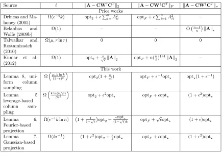
We have described these prior theoretical bounds in detail to emphasize how strong, relative to the prior work, our new bounds are. For example, Equation (4) provides an additive-error approximation with a very large scale; the bounds of Kumar, Mohri, and Talwalkar require a sampling complexity that depends on the coherence of the input matrix (Kumar et al., 2009a), which means that unless the coherence is very low one needs to sample essentially all the rows and columns in order to reconstruct the matrix; Equation (5) provides a bound where the additive scale depends onn; and Equation (6) provides a spectral norm bound where the scale of the additional error is the (much larger) trace norm. Table 1 compares the bounds on the approximation errors of SPSD sketches derived in this work to those available in the literature. We note further that Wang and Zhang recently established lower-bounds on the worst-case relative spectral and trace norm errors of uniform Nystr¨om extensions (Wang and Zhang, 2013). Our Lemma 8 provides matching upper bounds, showing the optimality of these estimates.

A related stream of research concerns projection-based low-rank approximations of gen-eral (i.e., non-SPSD) matrices (Halko et al., 2011; Mahoney, 2011). Such approximations are formed by first constructing an approximate basis for the top left invariant subspace of A, and then restricting A to this space. Algorithmically, one constructs Y = AS, where S is a sketching matrix, then takesQ to be a basis obtained from the QR decomposition of Y, and then forms the low-rank approximationQQTA.The survey paper Halko et al. (2011) proposes two schemes for the approximation of SPSD matrices that fit within this paradigm: Q(QTAQ)QT and (AQ)(QTAQ)†(QTA). The first scheme—for which Halko et al. (2011) provides quite sharp error bounds when Sis a matrix of i.i.d. standard Gaus-sian random variables—has the salutary property of being numerically stable. In Wang and Zhang (2013), the authors show that using the first scheme with an adaptively sampled S results in approximations with expected Frobenius error within a factor of 1 + of the optimal rank-kapproximation error when O(k/2) columns are sampled.

(9)

Source ` kA−CW†_CT_k

2 kA−CW†CTkF kA−CW†CTk?

Prior works Drineas and

Ma-honey (2005)

Ω(−4_k₎ _opt

2+

Pn

i=A2ii optF+

Pn

i=1A2ii –

Belabbas and

Wolfe (2009b)

Ω(1) – – O n−`

n

kAk_?

Talwalkar and

Rostamizadeh (2010)

Ω(µrrlnr) 0 0 0

Kumar et al.

(2012)

Ω(1) opt₂+_√n

`kAk2 optF+n(

k `)

1/4_k_A_k

2 –

This work

Lemma 8,

uni-form column

sampling

Ω

µkklnk (1−)2

opt₂(1 +_`n) opt_F+−1_opt

? opt?(1 +−1)

Lemma 5

leverage-based

column

sam-pling

Ω

kln(k/β)

β2

opt₂+2opt_? opt_F+opt_? (1 +2)opt_?

Lemma 6,

Fourier-based projection

Ω(−1_k_ln_n₎ _{1 +} 1

1−√

opt₂+ opt?

(1−√)k optF+

√

opt_? (1 +)opt_?

Lemma 7,

Gaussian-based projection

Ω(k−1₎ _{(1 +}2_)opt

2+kopt? optF+opt? (1 +2)opt?

Table 1: Comparison of our bounds on the approximation errors of several types of SPSD sketches with those provided in prior works. Only the asymptotically largest terms (as→0) are displayed and constants are omitted, for simplicity. Here,∈(0,1),

opt_ξ is the smallest ξ-norm error possible when approximating A with a rank-k

matrix (k≥lnn), r = rank(A), ` is the number of column samples sufficient for the stated bounds to hold,kis a target rank, andµsis the coherence ofArelative to the best rank-sapproximation toA.The parameterβ ∈(0,1] allows for the pos-sibility of sampling usingβ-approximate leverage scores (see Section 4.2.1) rather than the exact leverage scores. With the exception of (Drineas and Mahoney, 2005), which samples columns with probability proportional to their Euclidean norms, and our novel leverage-based Nystr¨om bound, these bounds are for sam-pling columns or linear combinations of columns uniformly at random. All bounds hold with constant probability.

(10)

(11)

source, sketch pred./obs. spectral error pred./obs. Frobenius error pred./obs. trace error

Enron,k= 60

Drineas and Mahoney (2005) nonuniform column sampling

3041.0 66.2 –

Belabbas and Wolfe (2009b) uniform column sampling

– – 2.0

Kumar et al. (2012) uniform column sampling

331.2 77.7 –

Lemma 5 leverage-based 1287.0 20.5 1.2

Lemma 6 Fourier-based 102.1 42.0 1.6

Lemma 7 Gaussian-based 20.1 7.6 1.4

Lemma 8 uniform column sampling

9.4 285.1 9.5

Protein,k= 10

Drineas and Mahoney (2005), nonuniform column sampling

125.2 18.6 –

Belabbas and Wolfe (2009b), uniform column sampling

– – 3.6

Kumar et al. (2012), uniform column sampling

35.1 20.5 –

Lemma 5, leverage-based 42.4 6.2 2.0

Lemma 6, Fourier-based 155.0 20.4 3.1

Lemma 7, Gaussian-based 5.7 5.6 2.2

Lemma 8, uniform column sampling

90.0 63.4 14.3

AbaloneD,σ=.15, k= 20

360.8 42.5 –

– – 2.0

62.0 45.7 –

13.2 166.2 9.0

WineS,σ= 1, k= 20

408.4 41.1 –

– – 2.1

70.3 44.3 –

13.2 162.2 9.1

(12)

2.5 An Overview of Our Bounds

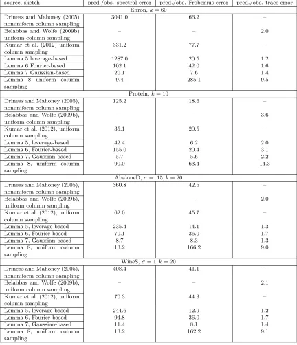
Our bounds in Table 1 (established as Lemmas 5–8 in Section 4.2) exhibit a common structure: for the spectral and Frobenius norms, we see that the additional error is on a larger scale than the optimal error, and the trace norm bounds all guarantee relative error approximations. This follows from the fact, as detailed in Section 4.1, that low-rank approximations that conform to the SPSD sketching model can be understood as forming column-sample/projection-based approximations to thesquare root ofA, and thus squaring this approximation yields the resulting approximation toA.The squaring process unavoidably results in potentially large additional errors in the case of the spectral and Frobenius norms— whether or not the additional errors are large in practice depends upon the properties of the matrix and the form of stochasticity used in the sampling process. For instance, from our bounds it is clear that Gaussian-based SPSD sketches are expected to have lower additional error in the spectral norm than any of the other sketches considered.

From Table 1, we also see, in the case of uniform Nystr¨om extensions, a necessary de-pendence on the coherence of the input matrix since columns are sampled uniformly at random. However, we also see that the scales of the additional error of the Frobenius and trace norm bounds are substantially improved over those in prior results. The large addi-tional error in the spectral norm error bound is necessary in the worse case (Gittens, 2012). Lemmas 5, 6 and 7 in Section 4.2—which respectively address leverage-based, Fourier-based, and Gaussian-based SPSD sketches—show that spectral norm additive-error bounds with additional error on a substantially smaller scale can be obtained if one first mixes the columns before sampling from A or one samples from a judicious nonuniform distribution over the columns.

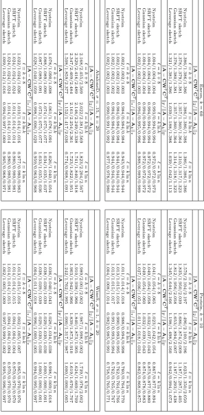
Table 2 compares the minimum, mean, and maximum approximation errors of several SPSD sketches of four matrices (described in Section 3.1) to the optimal rank-k approx-imation errors. We consider three regimes for `, the number of column samples used to construct the sketch: `= O(k), `= O(klnk),and `= O(klnn). These matrices exhibit a diverse range of properties: e.g., Enron is sparse and has a slowly decaying spectrum, while Protein is dense and has a rapidly decaying spectrum. Yet we notice that the sketches perform quite well on each of these matrices. In particular, when`= O(klnn),the average errors of the sketches are within 1 + of the optimal rank-k approximation errors, where

∈[0,1]. Also note that the leverage-based sketches consistently have lower average errors (in all of the three norms considered) than all other sketches. Likewise, the uniform Nystr¨om extensions usually have larger average errors than the other sketches. These two sketches represent opposite extremes: uniform Nystr¨om extensions (constructed using uniform col-umn sampling) are constructed using no knowledge about the matrix, while leverage-based sketches use an importance sampling distribution derived from the SVD of the matrix to determine which columns to use in the construction of the sketch.

(13)

sketches come quite close to capturing the errors seen in practice, and the Frobenius and trace norm error guarantees of the leverage-based and Fourier-based sketches tend to more closely reflect the empirical behavior than the error guarantees provided in prior work for Nystr¨om sketches. Overall, the trace norm error bounds are quite accurate. On the other hand, prior bounds are sometimes more informative in the case of the spectral norm (with the notable exception of the Gaussian sketches). Several important points can be gleaned from these observations. First, the accuracy of the Gaussian error bounds suggests that the main theoretical contribution of this work, the deterministic structural results given as Theorems 2 through 4, captures the underlying behavior of the SPSD sketching process. This supports our belief that this work provides a foundation for truly informative error bounds. Given that this is the case, it is clear that the analysis of the stochastic elements of the SPSD sketching process is much sharper in the Gaussian case than in the leverage-score, Fourier, and uniform Nystr¨om cases. We expect that, at least in the case of leverage and Fourier-based sketches, the stochastic analysis can and will be sharpened to produce error guarantees almost as informative as the ones we have provided for Gaussian-based sketches.

3. Empirical Aspects of SPSD Low-rank Approximation

In this section, we present our main empirical results, which consist of evaluating sampling and projection algorithms applied to a diverse set of SPSD matrices. The bulk of our empirical evaluation considers two random projection procedures and two random sampling procedures for the sketching matrix S: for random projections, we consider using SRFTs (Subsampled Randomized Fourier Transforms) as well as uniformly sampling from Gaussian mixtures of the columns; and for random sampling, we consider sampling columns uniformly at random as well as sampling columns according to a nonuniform importance sampling distribution that depends on the empirical statistical leverage scores. In the latter case of leverage score-based sampling, we also consider the use of both the (na¨ıve and expensive) exact algorithm as well as a (recently-developed fast) approximation algorithm. Section 3.1 starts with a brief description of the data sets we consider; Section 3.2 describes the details of our SPSD sketching algorithms; Section 3.3 summarizes our experimental results to help guide in the selection of sketching methods; in Section 3.4, we present our main results on reconstruction quality for the random sampling and random projection methods; and, in Section 3.5, we discuss running time issues, and we present our main results for running time and reconstruction quality for both exact and approximate versions of leverage-based sampling.

We emphasize that we don’t intend these results to be “comprehensive” but instead to be “illustrative” case-studies—that are representative of a much wider range of applications than have been considered previously. In particular, we would like to illustrate the tradeoffs between these methods in different realistic applications in order,e.g., to provide directions for future work. In addition to clarifying some of these issues, our empirical evaluation also illustrates ways in which existing theory is insufficient to explain the success of sampling and projection methods. This motivates our improvements to existing theory that we describe in Section 4.

(14)

comparisons, all computations were carried out in a single thread. When applied to an

n×nSPSD matrixA, our implementation of the SRFT requires O(n2lnn) operations, as it applies MATLAB’sfft to the entire matrix A and then it samples ` columns from the resulting matrix. A more rigorous implementation of the SRFT algorithm could reduce this running time to O(n2ln`), but due to the complexities involved in optimizing pruned FFT codes, we did not pursue this avenue.

3.1 Data Sets

Table 4 provides summary statistics for the data sets used in our empirical evaluation. We consider four classes of matrices commonly encountered in machine learning and data analysis applications: normalized Laplacians of very sparse graphs drawn from “informatics graph” applications; dense matrices corresponding to Linear Kernels from machine learning applications; dense matrices constructed from a Gaussian Radial Basis Function Kernel (RBFK); and sparse RBFK matrices constructed using Gaussian radial basis functions, truncated to be nonzero only for nearest neighbors. This collection of data sets represents a wide range of data sets with very different (sparsity, spectral, leverage score, etc.) prop-erties that have been of interest recently not only in machine learning but in data analysis more generally.

To understand better the Laplacian data, recall that, given an undirected graph with weighted adjacency matrix W, its normalized graph Laplacian is

A=I−D−1/2WD−1/2,

where D is the diagonal matrix of weighted degrees of the nodes of the graph, i.e., Dii =

P

j6=iWij.

The remaining data sets are kernel matrices associated with data drawn from a variety of application areas. Recall that, given given points x1, . . . ,xn ∈ Rd and a function κ : Rd×Rd→R,the n×n matrix with elements

Aij =κ(xi,xj)

is called the kernel matrix ofκ with respect to x1, . . . ,xn.Appropriate choices of κensure that A is positive semidefinite. When this is the case, the entries Aij can be interpreted as measuring, in a sense determined by the choice of κ, the similarity of points i and j. Specifically, if A is SPSD, then κ determines a so-called feature map Φκ : Rd → Rn such that

Aij =hΦκ(xi),Φκ(xj)i

measures the similarity (correlation) of xi and xj in feature space (Sch¨olkopf and Smola, 2001).

When κ is the usual Euclidean inner-product, so that

Aij =hxi,xki,

A is called a Linear Kernel matrix. Gaussian RBFK matrices, defined by

Aσ_ij = exp

_{− kxi}₋

xjk2₂

σ2

(15)

Name Description n d %nnz Laplacian Kernels

HEP arXiv High Energy Physics collaboration graph 9877 NA 0.06 GR arXiv General Relativity collaboration graph 5242 NA 0.12 Enron subgraph of the Enron email graph 10000 NA 0.22 Gnutella Gnutella peer to peer network on Aug. 6, 2002 8717 NA 0.09

Linear Kernels

Dexter bag of words 2000 20000 83.8

Protein derived feature matrix forS. cerevisiae 6621 357 99.7 SNPs DNA microarray data from cancer patients 5520 43 100 Gisette images of handwritten digits 6000 5000 100

Dense RBF Kernels

AbaloneD physical measurements of abalones 4177 8 100 WineD chemical measurements of wine 4898 12 100

Sparse RBF Kernels

AbaloneS physical measurements of abalones 4177 8 82.9/48.1 WineS chemical measurements of wine 4898 12 11.1/88.0

Table 4: The data sets used in our empirical evaluation (Leskovec et al., 2007; Klimt and Yang, 2004; Guyon et al., 2005; Gustafson et al., 2006; Nielsen et al., 2002; Corke, 1996; Asuncion and Newman, 2012). Here, n is the number of data points, d is the number of features in the input space before kernelization, and %nnz is the percentage of nonzero entries in the matrix. For Laplacian “kernels,” n is the number of nodes in the graph (and thus there is no d since the graph is “given” rather than “constructed”). The %nnz for the Sparse RBF Kernels depends on theσ parameter; see Table 5.

correspond to the similarity measure κ(x,y) = exp(−kx−yk2

2/σ2).Here σ, a nonnegative number, defines the scale of the kernel. Informally, σ defines the “size scale” over which pairs of points xi and xj “see” each other. Typically σ is determined by a global cross-validation criterion, as Aσ is generated for some specific machine learning task; and, thus, one may have noa priori knowledge of the behavior of the spectrum or leverage scores of Aσ asσ is varied. Accordingly, we consider Gaussian RBFK matrices with different values of σ.

Finally, given the same data points,x1, . . . ,xn, one can construct sparse Gaussian RBFK matrices

A(σ,ν,C_ij )=

1−kxi−xjk2

C

ν+

·exp

_{− kxi}₋

xjk2₂

σ2

,

(16)

Name %nnz lkAk

2 F

kAk2 2 m

k λk+1

λk 100

kA−AkkF

kAkF 100

kA−Akk? kAk?

kth-largest leverage score scaled byn/k

HEP 0.06 3078 20 0.998 7.8 0.4 128.8

HEP 0.06 3078 60 0.998 13.2 1.1 41.9

GR 0.12 1679 20 0.999 10.5 0.74 71.6

GR 0.12 1679 60 1 17.9 2.16 25.3

Enron 0.22 2588 20 0.997 7.77 0.352 245.8

Enron 0.22 2588 60 0.999 12.0 0.94 49.6

Gnutella 0.09 2757 20 1 8.1 0.41 166.2

Gnutella 0.09 2757 60 0.999 13.7 1.20 49.4

Dexter 83.8 176 8 0.963 14.5 .934 16.6

Protein 99.7 24 10 0.987 42.6 7.66 5.45

SNPs 100 3 5 0.928 85.5 37.6 2.64

Gisette 100 4 12 0.90 90.1 14.6 2.46

AbaloneD (dense,σ=.15) 100 41 20 0.992 42.1 3.21 18.11

AbaloneD (dense,σ= 1) 100 4 20 0.935 97.8 59 2.44

WineD (dense,σ= 1) 100 31 20 0.99 43.1 3.89 26.2

WineD (dense,σ= 2.1) 100 3 20 0.936 94.8 31.2 2.29

AbaloneS (sparse,σ=.15) 82.9 400 20 0.989 15.4 1.06 48.4

AbaloneS (sparse,σ= 1) 48.1 5 20 0.982 90.6 21.8 3.57

WineS (sparse,σ= 1) 11.1 116 20 0.995 29.5 2.29 49.0

WineS (sparse,σ= 2.1) 88.0 39 20 0.992 41.6 3.53 24.1

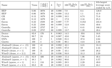
Table 5: Summary statistics for the data sets from Table 4 that we used in our empirical evaluation.

A(σ,ν,C) approaches the (dense) Gaussian RBFK matrixAσ.For simplicity, in our empirical evaluations, we fix ν =d(d+ 1)/2e andC = 3σ, and we vary σ.

To illustrate the diverse range of properties exhibited by these four classes of data sets, consider Table 5. Several observations are particularly relevant to our discussion below.

• All of the Laplacian Kernels drawn from informatics graph applications are extremely sparse in terms of number of nonzeros, and they all tend to have very slow spectral decay, as illustrated both by the quantity kAk2_F/kAk2₂

(this is the stable rank, which is a numerically stable (under)estimate of the rank of A) as well as by the relatively small fraction of the Frobenius norm that is captured by the best rank-k

approximation toA.

(17)

• For the Dense RBF Kernels, we consider two values of theσ parameter, again chosen (somewhat) arbitrarily. For both AbaloneD and WineD, we see that decreasingσfrom 1 to 0.15,i.e., letting data points “see” fewer nearby points, has two important effects: first, it results in matrices that are muchless well-approximated by low-rank matrices; and second, it results in matrices that havemuch more heterogeneous leverage scores.

• For the Sparse RBF Kernels, there are a range of sparsities, ranging from above the sparsity of the sparsest Linear Kernel, but all are denser than the Laplacian Kernels. Changing theσ parameter has the same effect (although it is even more pronounced) for Sparse RBF Kernels as it has for Dense RBF Kernels. In addition, “sparsifying” a Dense RBF Kernel also has the effect of making the matrix less well approximated by a low-rank matrix and of making the leverage scores more nonuniform.

As we see below, when we consider the RBF Kernels as the width parameter and sparsity are varied, we observe a range of intermediate cases between the extremes of the (“nice”) Linear Kernels and the (very “non-nice”) Laplacian Kernels.

3.2 SPSD Sketching Algorithms

The sketching matrix Smay be selected in a variety of ways. For sampling-based sketches, the sketching matrix S contains exactly one nonzero in each column, corresponding to a single sample from the columns ofA.For projection-based sketches,S is dense, and mixes the columns of Abefore sampling from the resulting matrix.

In more detail, we consider two types of sampling-based SPSD sketches (i.e. Nystr¨om extensions): those constructed by sampling columns uniformly at random with replacement, and those constructed by sampling columns from a distribution based upon the leverage scores of the matrix filtered through the optimal rank-k approximation of the matrix. In the case of column sampling, the sketching matrixSis simply the first`columns of a matrix that was chosen uniformly at random from the set of all permutation matrices.

In the case of leverage-based sampling, S has a more complicated distribution. Recall that the leverage scores relative to the best rank-k approximation to A are the squared Euclidean norms of the rows of then×k matrixU1 :

`j =k(U1)jk2.

It follows from the orthonormality ofU1thatPj(`j/k) = 1,and the leverage scores can thus be interpreted as a probability distribution over the columns ofA.To construct a sketching matrix corresponding to sampling from this distribution, we first select the columns to be used by sampling with replacement from this distribution. Then, S is constructed as S=RDwhereR∈_Rn×` _{is a column selection matrix that samples columns of}_A_{from the} given distribution—i.e., Rij = 1 iff the ith column of A is the jth column selected—and D is a diagonal rescaling matrix satisfyingDjj = √1_`p

i iff Rij = 1. Here, pi =`i/k is the

probability of choosing the ith column of A.It is often expensive to compute the leverage scores exactly; in Section 3.5, we consider the performance of sketches based on several leverage score approximation algorithms.

(18)

S is a subsampled randomized Fourier transform (SRFT) matrix; that is, S = p_n

`DFR, whereD is a diagonal matrix of Rademacher random variables,Fis the real Fourier trans-form matrix, andR restricts to`columns.

For conciseness, we do not present results for sampling-based sketches where rows are selected with probability proportional to their row norms. This form of sampling can be similar to leverage-score sampling for sparse graphs with highly connected vertices (Ma-honey and Drineas, 2009), and in cases where the matrix has been preprocessed to have uniform row lengths, reduces to uniform sampling.

In the figures, we refer to sketches constructed by selecting columns uniformly at ran-dom with the label ‘unif’, leverage score-based sketches with ‘lev’, Gaussian sketches with ‘gaussian’, and Fourier sketches with ‘srft’.

3.3 Guidelines for Selecting Sketching Schemes

In the remainder of this section of the paper, we provide empirical evaluations of the sam-pling and projection-based sketching schemes just described, with an eye towards identifying the aspects of the datasets that affect the relative performance of the sketching schemes. However our experiments also provide some practical guidelines for selecting a particular sketching scheme.

• Despite the theoretical result that the worst-case spectral error in using Nystr¨om sketches obtained via uniform column-samples can be much worse than that of using projection or leverage-based sketches, on the corpus of data sets we considered, such sketches perform within a small multiple of the error of more computationally expen-sive leverage-based and projection-based sketches. For data sets with more nonuni-form leverage score properties, random projections and leverage-based sampling will do better (Ma et al., 2014).

• In the case where parsimony of the sketch is of primary concern, i.e. where the primary concern is to maintain ` ≈ k, leverage sketches are an attractive option. In particular, when an RBF kernel with small bandwidth is used, or the data set is sparse, leverage-based sketches often provide higher accuracy than projection or uniform-sampling based sketches.

• The norm in which the error is measured should be taked into consideration when selecting the sketching algorithm. In particular, sketches which use power iterations are most useful when the error is measured in the spectral norm, and in this case, projection-based sketches (in particular, prolonged sketches– see Section 3.6) notice-ably outperform uniform sampling-based sketches.

3.4 Reconstruction Accuracy of Sampling and Projection Algorithms

(19)

turn, and then we summarize our observations. We consider only the use of exact leverage scores here, and we postpone until Section 3.5 a discussion of running time issues and sim-ilar reconstruction results when approximate leverage scores are used for the importance sampling distribution. The relative errors

A−CW

†_CT

ξ/

kA−Akkξ (7)

are plotted, with each point in the figures of this section representing the average errors observed over 30 trials.

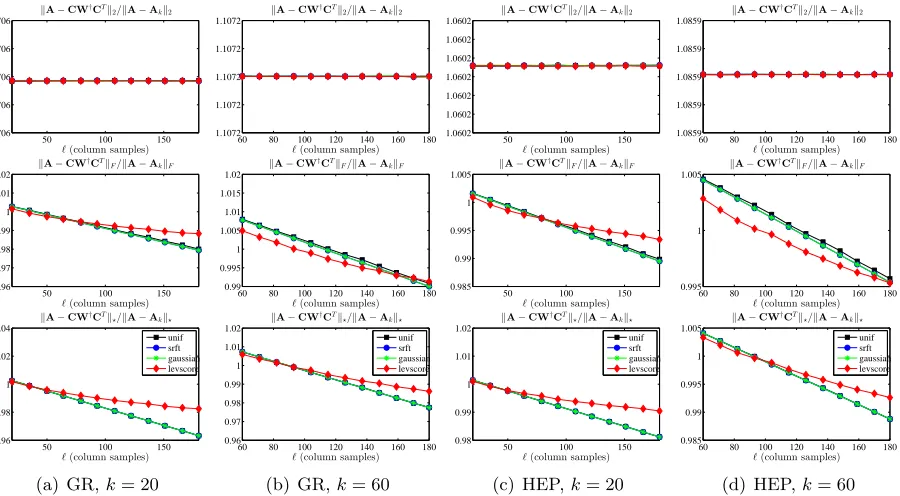
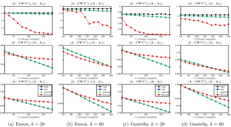
3.4.1 Graph Laplacians

Figure 1 and Figure 2 show the reconstruction error results for sampling and projection methods applied to several normalized graph Laplacians. The former shows GR and HEP, each for two values of the rank parameter, and the latter shows Enron and Gnutella, again each for two values of the rank parameter. Both figures show the spectral, Frobenius, and trace norm approximation errors, as a function of the number of column samples`, relative to the error of the optimal rank-kapproximation of A.

50 100 150 1.0706

1.0706 1.0706 1.0706 1.0706

`(column samples) kA₋CW†CT_k

2/kA₋Akk2

50 100 150 0.96

0.97 0.98 0.99 1 1.01 1.02

F/kA−AkkF

50 100 150 0.96

0.98 1 1.02 1.04

`(column samples) kA

−CW†CTk?/kA−Akk?

unif srft gaussian levscore

(a) GR,k= 20

60 80 100 120 140 160 180 1.1072

1.1072 1.1072 1.1072 1.1072

2/kA₋Akk2

60 80 100 120 140 160 180 0.99

0.995 1 1.005 1.01 1.015 1.02

F/kA−AkkF

60 80 100 120 140 160 180 0.96

0.97 0.98 0.99 1 1.01 1.02

(b) GR,k= 60

50 100 150 1.0602

1.0602 1.0602 1.0602 1.0602 1.0602 1.0602

2/kA₋Akk2

50 100 150 0.985

0.99 0.995 1 1.005

`(column samples) kA₋CW†CT_k_F/_kA₋A_k_k_F

50 100 150 0.98

0.99 1 1.01 1.02

(c) HEP,k= 20

60 80 100 120 140 160 180 1.0859

1.0859 1.0859 1.0859 1.0859

2/kA₋Akk2

60 80 100 120 140 160 180 0.995

1 1.005

60 80 100 120 140 160 180 0.985

0.99 0.995 1 1.005

(d) HEP,k= 60

(20)

50 100 150 1

1.1 1.2 1.3 1.4

2/kA₋Akk2

50 100 150 0.99

0.995 1 1.005

F/kA−AkkF

50 100 150 0.98

0.99 1 1.01 1.02

(a) Enron,k= 20

60 80 100 120 140 160 180 1.25

1.3 1.35 1.4

2/kA₋Akk2

60 80 100 120 140 160 180 0.995

1 1.005

F/kA−AkkF

60 80 100 120 140 160 180 0.99

0.995 1 1.005

(b) Enron,k= 60

50 100 150 1

1.02 1.04 1.06 1.08 1.1

2/kA₋Akk2

50 100 150 0.985

0.99 0.995 1 1.005

50 100 150 0.98

0.99 1 1.01 1.02

(c) Gnutella,k= 20

60 80 100 120 140 160 180 1

1.05 1.1 1.15

2/kA₋Akk2

60 80 100 120 140 160 180 0.995

1 1.005 1.01 1.015

60 80 100 120 140 160 180 0.985

0.99 0.995 1 1.005

(d) Gnutella,k= 60

Figure 2: The spectral, Frobenius, and trace norm errors (top to bottom, respectively, in each subfigure) of several SPSD sketches, as a function of the number of column samples`, for the Enron and Gnutella Laplacian data sets, with two choices of the rank parameterk.

These and subsequent figures contain a lot of information, some of which is peculiar to the given data sets and some of which is more general. In light of subsequent discussion, several observations are worth making about the results presented in these two figures.

• All of the SPSD sketches provide quite accurate approximations—relative to the best possible approximation factor for that norm, and relative to bounds provided by existing theory, as reviewed in Section 2.4—even with only k column samples (or in the case of the Gaussian and SRFT mixtures, with only k linear combinations of columns). Upon examination, this is partly due to the extreme sparsity and extremely slow spectral decay of these data sets which means, as shown in Table 4, that only a small fraction of the (spectral or Frobenius or trace) mass is captured by the optimal rank 20 or 60 approximation. Thus, although an SPSD sketch constructed from 20 or 60 vectors also only captures a small portion of the mass of the matrix, the relative error is small, since the scale of the residual error is large.

(21)

GR k= 20 with GR k= 60. This is also consistent with the larger amount of mass captured by higher-rank approximations.

• For ` > k, the errors tend to decrease (or at least not increase, as for GR and HEP

the spectral norm error is flat as a function of `), which is intuitive.

• The X axes ranges from kto 9k for thek= 20 plots and from kto 3k for thek= 60 plots. As a practical matter, choosing ` between k and (say) 2k or 3k is probably of greatest interest. In this regime, there is an interesting tradeoff: for moderately large values of ` in this regime, the error for leverage-based sampling is moderately better than for uniform sampling or random projections, while if one chooses `to be much larger then the improvements from leverage-based sampling saturate and the uniform sampling and random projection methods are better. This is most obvious in the Frobenius norm plots, although it is also seen in the trace norm plots, and it suggests that some combination of leverage-based sampling and uniform sampling might be best.

• The behavior of the approximations with respect to the spectral norm is quite different from the behavior in the Frobenius and trace norms. In the latter, as the number of samples`increases, the errors tend to decrease; while for the former, the errors tend to be much flatter as a function of increasing`for at least the Gaussian, SRFT, and uniformly sampled sketches.

All in all, there seems to be quite complicated behavior for low-rank sketches for these Laplacian data sets. Several of these observations can also be made for subsequent figures; but in some other cases the (very sparse and not very low rank) structural properties of the data are primarily responsible.

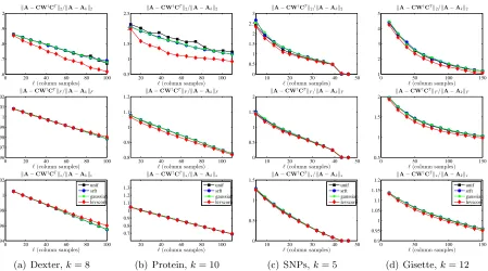
3.4.2 Linear Kernels

Figure 3 shows the reconstruction error results for sampling and projection methods applied to several Linear Kernels. The data sets (Dexter, Protein, SNPs, and Gisette) are all quite low-rank and have fairly uniform leverage scores. Several observations are worth making about the results presented in this figure.

• All of the methods perform quite similarly: all have errors that decrease smoothly with increasing `, and in this case there is little advantage to using methods other than uniform sampling (since they perform similarly and are more expensive). Also, since the ranks are so low and the leverage scores are so uniform, the leverage score sketch is no longer significantly distinguished by its tendency to saturate quickly.

• The scale of the Y axes is much larger than for the Laplacian data sets, mostly since the matrices are much more well-approximated by low-rank matrices, although the scale decreases as one goes from spectral to Frobenius to trace reconstruction error, as before.

These linear kernels (and also to some extent the dense RBF kernels below that have larger

(22)

0 20 40 60 80 100 1.6

1.7 1.8 1.9 2

2/kA₋Akk2

0 20 40 60 80 100 0.96

0.97 0.98 0.99 1 1.01 1.02

F/kA−AkkF

0 20 40 60 80 100 0.94

0.96 0.98 1 1.02

(a) Dexter,k= 8

20 40 60 80 100 0.5

1 1.5 2 2.5

2/kA₋Akk2

20 40 60 80 100 0.8

0.9 1 1.1 1.2

F/kA−AkkF

20 40 60 80 100 0.7

0.8 0.9 1 1.1 1.2 1.3

(b) Protein,k= 10

10 20 30 40 50 0

0.5 1 1.5 2 2.5 3

2/kA₋Akk2

10 20 30 40 50 0

0.5 1 1.5 2

10 20 30 40 50 0

0.5 1 1.5

(c) SNPs,k= 5

0 50 100 150

1 2 3 4 5

2/kA₋Akk2

0 50 100 150

0.5 1 1.5 2

0 50 100 150

0.9 0.95 1 1.05 1.1 1.15 1.2

(d) Gisette,k= 12

Figure 3: The spectral, Frobenius, and trace norm errors (top to bottom, respectively, in each subfigure) of several SPSD sketches, as a function of the number of column samples`, for the Linear Kernel data sets.

to matrices where uniform sampling has been shown to perform well previously (Talwalkar et al., 2008; Kumar et al., 2009a,c, 2012); for these matrices our empirical results agree with these prior works.

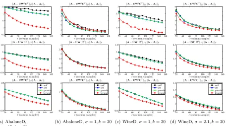
3.4.3 Dense and Sparse RBF Kernels

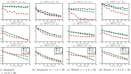
Figure 4 and Figure 5 present the reconstruction error results for sampling and projection methods applied to several dense RBF and sparse RBF kernels. Several observations are worth making about the results presented in these figures.

• All of the methods have errors that decrease with increasing`, but for larger values ofσ

and for denser data, the decrease is somewhat more regular, and the four methods tend to perform similarly. For larger values ofσ and sparser data, leverage score sampling is somewhat better. This parallels what we observed with the Linear Kernels, except that here the leverage score sampling is somewhat better for all values of `.

(23)

20 40 60 80 100 120 140 160 0.5

1 1.5 2 2.5

2/kA₋Akk2

20 40 60 80 100 120 140 160 0.95

1 1.05 1.1 1.15

F/kA−AkkF

20 40 60 80 100 120 140 160 0.95

1 1.05

(a) AbaloneD, σ=.15, k= 20

20 40 60 80 100 120 140 160 0

1 2 3 4 5 6

2/kA₋Akk2

20 40 60 80 100 120 140 160 0

0.5 1 1.5 2 2.5 3

F/kA−AkkF

20 40 60 80 100 120 140 160 0.5

1 1.5 2

(b) AbaloneD,σ= 1, k= 20

20 40 60 80 100 120 140 160 1

1.5 2 2.5 3

2/kA₋Akk2

20 40 60 80 100 120 140 160 0.95

1 1.05 1.1 1.15

20 40 60 80 100 120 140 160 0.95

1 1.05

(c) WineD,σ= 1, k= 20

20 40 60 80 100 120 140 160 0

1 2 3 4 5 6

2/kA₋Akk2

20 40 60 80 100 120 140 160 0.5

1 1.5 2 2.5

20 40 60 80 100 120 140 160 0.8

1 1.2 1.4 1.6

(d) WineD,σ= 2.1, k= 20

Figure 4: The spectral, Frobenius, and trace norm errors (top to bottom, respectively, in each subfigure) of several SPSD sketches, as a function of the number of column samples`, for several dense RBF data sets.

Recall from Table 5 that for smaller values ofσ and for sparser kernels, the SPSD matrices are less well-approximated by low-rank matrices, and they have more heterogeneous leverage scores. Thus, they are more similar to the Laplacian data than the Linear Kernel data; this suggests (as we have observed) that leverage score sampling should perform relatively better than uniform column sampling and projection-based schemes when in these two cases.

3.4.4 Summary of Comparison of Sampling and Projection Algorithms

Before proceeding, there are several summary observations that we can make about sampling versus projection methods for the data sets we have considered.

• Linear Kernels and to a lesser extent Dense RBF Kernels with larger σ parameter have relatively low rank and relatively uniform leverage scores, and in these cases uniform sampling does quite well. These data sets correspond most closely with those that have been studied previously in the machine learning literature, and for these data sets our results are in agreement with that prior work.

(24)

20 40 60 80 100 120 140 160 0.5

1 1.5 2

2/kA₋Akk2

20 40 60 80 100 120 140 160 0.99

0.995 1 1.005 1.01 1.015 1.02

F/kA−AkkF

20 40 60 80 100 120 140 160 0.96

0.97 0.98 0.99 1 1.01 1.02

(a) AbaloneS, σ=.15, k= 20

20 40 60 80 100 120 140 160 0

1 2 3 4 5 6

2/kA₋Akk2

20 40 60 80 100 120 140 160 0.5

1 1.5 2

F/kA−AkkF

20 40 60 80 100 120 140 160 0.9

1 1.1 1.2 1.3

(b) AbaloneS,σ= 1, k= 20

20 40 60 80 100 120 140 160 1

1.5 2 2.5

2/kA₋Akk2

20 40 60 80 100 120 140 160 0.95

1 1.05 1.1

20 40 60 80 100 120 140 160 0.96

0.98 1 1.02 1.04

(c) WineS,σ= 1, k= 20

20 40 60 80 100 120 140 160 1

1.5 2 2.5

2/kA₋Akk2

20 40 60 80 100 120 140 160 0.95

1 1.05 1.1 1.15

20 40 60 80 100 120 140 160 0.95

1 1.05

(d) WineS,σ= 2.1, k= 20

Figure 5: The spectral, Frobenius, and trace norm errors (top to bottom, respectively, in each subfigure) of several SPSD sketches, as a function of the number of column samples`, for several sparse RBF data sets.

eigenvectors—but for the data we examined they are related, in that matrices with more slowly decaying spectra also often have more heterogeneous leverage scores.

• For Dense RBF Kernels with smaller σ and Sparse RBF Kernels, leverage score sampling tends to do much better than other methods. Interestingly, the Sparse RBF Kernels have many properties of very sparse Laplacian Kernels corresponding to relatively-unstructured informatics graphs, an observation which should be of inter-est for researchers who construct sparse graphs from data using,e.g., “locally linear” methods, to try to reconstruct hypothesized low-dimensional manifolds.

• Reconstruction quality under leverage score sampling saturates, as a function of choos-ing more samples`. As a consequence, there can be a tradeoff between leverage score sampling or other methods being better, depending on the values of`that are chosen.

(25)

randomly-rotated basis where the leverage scores have been approximately uniformized (Ma-honey, 2011)) is very much tied to the Frobenius norm, and so there is noa priorireason to expect its good performance to extend to the spectral or trace norms. Motivated by this, we revisit the question of proving improved worst-case theoretical bounds in Section 4.

Before describing these improved theoretical results, however, we address in Section 3.5 running time questions. After all, a na¨ıve implementation of sampling with exact leverage scores is slower than other methods (and much slower than uniform sampling). As shown below, by using the recently-developed approximation algorithm of Drineas et al. (2012), not only does this approximation algorithm run in time comparable with random projections (for certain parameter settings), it also leads to approximations that soften the strong bias that the exact leverage scores provide toward the best rank-kapproximation to the matrix, thereby leading to improved reconstruction results in many cases.

3.5 Reconstruction Accuracy of Leverage Score Approximation Algorithms

A na¨ıve view might assume that computing probabilities that permit leverage-based sam-pling requires an O(n3) computation of the full SVD, or at least the full computation of a partial SVD, and thus that it would be much more expensive than recently-developed random projection methods. Indeed, an “exact” computation of the leverage scores with a truncated SVD takes roughly O(n2k) time. Recent work, however, has shown that relative-error approximations to all the statistical leverage scores can be computed more quickly than this exact algorithm (Drineas et al., 2012). Here, we implement and evaluate a version of this algorithm. We evaluate it both in terms of running time and in terms of reconstruc-tion quality on the diverse suite of real data matrices we considered above. This is the first work to provide an empirical evaluation of an implementation of the leverage score approx-imation algorithms of Drineas et al. (2012), illustrating empirically the tradeoffs between cost and efficiency in a practical setting.

3.5.1 Description of the Fast Approximation Algorithm of Drineas et al. (2012)

Algorithm 1 (which originally appeared as Algorithm 1 in Drineas et al. (2012)) takes as input an arbitrary n×d matrix A, where n d, and it returns as output a 1±

approximation to all of the statistical leverage scores of the input matrix. The original algorithm of Drineas et al. (2012) uses a subsampled Hadamard transform and requires r1 to be somewhat larger than what we state in Algorithm 1. That an SRFT with a smaller value ofr1can be used instead is a consequence of the fact that (Drineas et al., 2012, Lemma 3) is also satisfied by an SRFT matrix with the givenr1; this is established in (Tropp, 2011; Boutsidis and Gittens, 2013).

The running time of this algorithm, given in the caption of the algorithm, is roughly

(26)

Input: A∈Rn×d (with SVD A=UΣVT), error parameter∈(0,1/2]. Output: `˜i, i= 1, . . . , n, approximations to the leverage scores of A.

1. Let Π1 ∈Rr1×n be an SRFT with

r1 = Ω(−2( √

d+

√

lnn)2lnd)

2. Compute Π1A∈Rr1×d and its QR factorization Π1A=QR.

3. Let Π2 ∈Rd×r2 be a matrix of i.i.d. standard Gaussian random variables, where

r2 = Ω −2lnn

.

4. Construct the productΩ=AR−1Π2.

5. For i= 1, . . . , n compute ˜`i =

Ω_(i)

2 2.

Algorithm 1:Algorithm (Drineas et al., 2012, Algorithm 1) for approximating the lever-age scores`i of ann×dmatrixA, wherend, to within a multiplicative factor of 1±. The running time of the algorithm is O(ndln(√d+√lnn) +nd−2lnn+d2−2(√d+ √

lnn)2lnd).

the leverage scores from the Euclidean norms of the rows. Of course, computing the QR decomposition would require O(nd2) time. To get around this, Algorithm 1 premultiplies A by a structured random projection Π1, computes a QR decomposition of Π1A, and postmultiplies A by R−1, i.e., the inverse of the “R” matrix from the QR decomposition of Π1A. Since Π1 is an SRFT, premultiplying by it takes roughly O(ndlnd) time. In addition, note that Π1A needs to be post multiplied by a second random projection in order to compute all of the leverage scores in the allotted time; see (Drineas et al., 2012) for details. This algorithm is simpler than the algorithm in which we are primarily interested that is applicable to square SPSD matrices, but we start with it since it illustrates the basic ideas of how our main algorithm works and since our main algorithm calls it as a subroutine. We note, however, that this algorithm is directly useful for approximating the leverage scores of Linear Kernel matricesA=XXT, when Xis a tall and skinny matrix.

(27)

Input: A∈Rn×d,a rank parameterk,and an error parameter∈(0,1/2]. Output: `ˆi, i= 1, . . . , n, approximations to the leverage scores of Afiltered through its dominant dimension-ksubspace.

1. Construct Π∈_Rd×2k _{with i.i.d. standard Gaussian entries.} 2. Compute B= AATqAΠ∈Rn×2k with

q ≥



   

ln

1 +

q

k k−1 + e

q

2 k

p

min{n, d} −k

2 ln (1 +/10)−1/2



    .

3. Approximate the leverage scores of Bby calling Algorithm 1 with inputs B and ; let ˆ`i fori= 1, . . . , n be the outputs of Algorithm 1.

Algorithm 2:Algorithm (Drineas et al., 2012, Algorithm 4) for approximating the lever-age scores (relative to the best rank-k approximation to A) of a general n×d matrix A with those of a matrix that is close by in the spectral norm (or the Frobenius norm if q = 0). This algorithm runs in time O(ndkq) +T1, where T1 is the running time of Algorithm 1.

a matrix close to Ain the Frobenius norm or spectral norm, and then it approximates the leverage scores of this matrix by using Algorithm 1 on the smaller, very rectangular matrix B. When A is square, as in our applications, Algorithm 2 is typically more costly than direct computation of the leverage scores, at least for dense matrices (but it does have the advantage that the number of iterations is bounded, independent of properties of the matrix, which is not true for typical iterative methods to compute low-rank approximations).

Of greater practical interest is Algorithm 3, which is a modification of Algorithm 2 in which the Gaussian random projection is replaced with an SRFT. That is, Algorithm 3 uses an SRFT projection to find a matrix close by toA in the Frobenius norm or spectral norm (depending on the value ofq), and then it exactly computes the leverage scores of this matrix. This improves the running time to O(n2ln(√k+√lnn) +n2(√k+√lnn)2ln(k)q+

n(√k+√lnn)4_ln2₍_k₎₎_, _{which is} _o₍_n2_k_{) when} _q _{= 0. Thus an important point for} Al-gorithm 3 (as well as for AlAl-gorithm 2) is the parameter q which describes the number of iterations. For q = 0 iterations, we get an inexpensive Frobenius norm approximation; while for higher q, we get better spectral norm approximations that are more expensive.3 This flexibility is of interest, as one may want to approximate the actual leverage scores accurately or one may simply want to find crude approximations useful for obtaining SPSD sketches with low reconstruction error.

3. Observe that since Ais rectangular in Algorithms 2 and 3, we approximate the leverage scores of A

(28)

Input: A∈Rn×d, a rank parameterk, and an iteration parameter q.

Output: `ˆi, i∈= 1, . . . , n,approximations to the leverage scores of Afiltered through its dominant dimension-ksubspace.

1. Construct an SRHT matrixΠ∈_Rd×r_,_where

r≥l36−2[ √

k+p8 ln(kd)]2ln(k)

m .

2. Compute B= AATqAΠ∈Rn×r,whereq≥0 is an integer. 3. Return the exact leverage scores of B.

Algorithm 3: Algorithm for approximating the leverage scores (relative to the best rank-k approximation to A) of a general n×d matrix A with those of a matrix that is close by in the spectral norm. This is a modified version of Algorithm 2, in which the random projection is implemented with an SRFT rather than a Gaussian random matrix, and where the number of “iterations” q is prespecified. This algorithm runs in time O(ndlnr+ndrq+nr2) since AΠcan be computed in time O(ndlnr).

Finally, note that although choosing the number of iterationsqas we did in Algorithm 2 is convenient for worst-case analysis, as a practical implementational matter it is easier either to chooseq based on spectral gap information revealed during the running of the algorithm or to prespecify q to be a small integer, e.g., 2 or 3, before the algorithm runs. Both of these have an interpretation of accelerating the rate of decay of the spectrum with a power iteration, but they behave somewhat differently due to the different stopping conditions. Below, we consider both variants.

3.5.2 Running Time Comparisons

Here, we describe the performances of the various random sampling and random projection low-rank sketches considered in Section 3.4 in terms of their running time, where the method that involves using the leverage scores to construct the importance sampling distribution is implemented both by computing the leverage scores “exactly” by calling a truncated SVD, as a black box, as well as computing them approximately by using one of several versions of Algorithm 3. Our running time results are presented in Figure 6 and Figure 7.