Superior Guarantees for Sequential Prediction and Lossless Compression via Alphabet Decomposition

Superior Guarantees for Sequential Prediction

and Lossless Compression via Alphabet Decomposition

Ron Begleiter [email protected]

Ran El-Yaniv [email protected]

Department of Computer Science Technion - Israel Institute of Technology Haifa 32000, Israel

Editor: Dana Ron

Abstract

We present worst case bounds for the learning rate of a known prediction method that is based on hierarchical applications of binary context tree weighting (CTW) predictors. A heuristic application of this approach that relies on Huffman’s alphabet decomposition is known to achieve state-of-the-art performance in prediction and lossless compression benchmarks. We show that our new bound for this heuristic is tighter than the best known performance guarantees for prediction and lossless compression algorithms in various settings. This result substantiates the efficiency of this hierarchical method and provides a compelling explanation for its practical success. In addition, we present the results of a few experiments that examine other possibilities for improving the multi-alphabet prediction performance of CTW-based algorithms.

Keywords: sequential prediction, the context tree weighting method, variable order Markov

mod-els, error bounds

1. Introduction

Sequence prediction and entropy estimation are fundamental tasks in numerous machine learning and data mining applications. Here we consider a standard discrete sequence prediction setting where performance is measured via the log-loss (self-information). It is well known that this setting is intimately related to lossless compression, where in fact high quality prediction is essentially equivalent to high quality lossless compression.

Despite the major interest in sequence prediction and the existence of a number of universal prediction algorithms, some fundamental issues related to learning from finite (and small) samples are still open. One issue that motivated the current research is that the finite-sample behavior of prediction algorithms is still not sufficiently understood.

Among the numerous compression and prediction algorithms there are very few that offer both finite sample guarantees and good practical performance. The context tree weighting (CTW) method

The high practical performance of the originalCTWalgorithm is most apparent when applied to

binary prediction problems, in which case it uses the well-known (binary) KT-estimator (Krichevsky

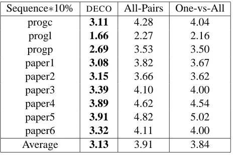
and Trofimov, 1981). When the algorithm is applied to non-binary prediction/compression problems (using the multi-alphabet KT-estimator), its empirical performance is mediocre compared to the best known results (Tjalkens et al., 1997). Nevertheless, a clever alphabet decomposition heuristic, sug-gested by Tjalkens et al. (1994) and further developed by Volf (2002), does achieve state-of-the-art compression and prediction performance on standard benchmarks (see, e.g., Volf, 2002; Sadakane et al., 2000; Shkarin, 2002; Begleiter et al., 2004). In this approach the multi-alphabet problem is hierarchically decomposed into a number of binary prediction problems. We term the resulting procedure “the DECO algorithm.” Volf suggested applying the DECO algorithm using Huffman’s

tree as the decomposition structure, where the tree construction is based on letter frequencies. We are not aware of any previous compelling explanation for the striking empirical success ofDECO.

Our main contribution is a general worst case redundancy bound for algorithm DECO applied

with any alphabet decomposition structure. The bound proves that the algorithm is universal with respect to VMMs. A specialization of the bound to the case of Huffman decompositions results in a tight redundancy bound. To the best of our knowledge, this new bound is the sharpest available for prediction and lossless compression for sufficiently large alphabets and sequences.

We also present a few empirical results that provide some insight into the following questions: (1) Can we improve on the Huffman decomposition structure using an optimized decomposition tree? (2) Can other, perhaps “flat” types of alphabet decomposition schemes outperform the hierar-chical approach? (3) Can standardCTWmulti-alphabet prediction be improved with other types of (non-KT) zero-order estimators?

Before we start with the technical exposition, we introduce some standard terms and definitions. Throughout the paper, Σ denotes a finite alphabet with k=_|Σ_| symbols. Suppose we are given a sequence xn₁=x1x2···xn. Our goal is to generate a probabilistic prediction ˆP(xn+1|xn1) for the

next symbol given the previous symbols. Clearly this is equivalent to being able to estimate the probability ˆP(xn₁)of any complete sequence, since ˆP(xn+1|xn1) =Pˆ(x

n+1

1 )/Pˆ(xn1)(provided that the

marginality condition∑_σPˆ(xn₁σ) =_Pˆ_(xn

1)holds).

We consider a setting where the performance of the prediction algorithm is measured with re-spect to the best predictor in some reference, which we call here a comparison class. In our case the comparison class is the set of all variable order Markov models (see details below). LetALGbe a prediction algorithm that assigns a probability estimate PALG(xn₁) for any given xn₁. The

point-wise redundancy of ALG with respect to the predictor P and the sequence xn₁ is RALG(xn₁,P) = log P(xn₁)₋log PALG(xn₁). The per-symbol point-wise redundancy is 1

nRALG(x n

1,P). ALGis called universal with respect to a comparison class

C

_{, if}

lim n→∞_Psup_∈C

max xn

1 1

nRALG(x

n

1,P) =0. (1)

2. Preliminaries

This section presents the relevant technical background for the present work. The contextual back-ground appears in Section 7. We start by presenting the class of tree sources. We then describe theCTWalgorithm and discuss some of its known properties and performance guarantees. Finally,

2.1 Tree Sources

The parametric distribution estimated by the CTW algorithm is the set of depth-bounded tree-sources. A tree-source is a variable order Markov model (VMM). Let Σ be an alphabet of size

k and D a non-negative integer. A D-bounded tree source is any full k-ary tree1whose height_≤D.

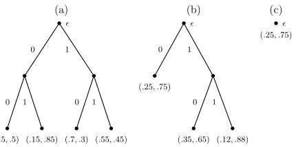
Each leaf of the tree is associated with a probability distribution overΣ. For example, in Figure 1 we depict three tree-sources over a binary alphabet. In this case, the trees are full binary trees. The single node tree in Figure 1(c) is a zero-order (Bernoulli) source and the other two trees (Figure 1(a) and (b)) are 2-bounded sources. Another useful way to view a tree-source is as a set

S

_⊆Σ≤D_of “suffixes” in which each s_∈

S

is a path (of length up to D) from a (unique) leaf to the root. We also refer to

S

_{as the (tree-source) topology. For example,}

S

_={0,01,11_}in Figure 1(b). The path from the middle leaf to the root corresponds to the sequence s=01and therefore we refer to this leaf simply as s. For convenience we also refer to an internal node by the (unique) path from that node to the root. Observe that this path is a suffix of some s∈

S

_{. For example, the right child of the root} in Figure 1(b) is denoted by the suffix1.

The (zero-order) distribution associated with the leaf s is denoted zs(σ),∀σ∈Σ, where∑σzs(σ) = 1 and zs(·)≥0.

(a) (b) (c)

²

0

(.5, .5) 0

(.15, .85) 1

1

(.7, .3) 0

(.55, .45) 1

²

(.25, .75)

0 1

(.35, .65) 0

(.12, .88) 1

²

(.25, .75)

Figure 1: Three examples for D =2 bounded tree-sources over Σ=_{0,1_}. The correspond-ing suffix-sets are

S

_(a)=_{00,10,01,11_},

S

_(b)=_{0,01,11_}, and

S

_(c) =_{ε_} (ε is the empty sequence). The probabilities for generating x3₁ =100 given initial context 00 are P₍a)(100|00) =P(a)(1|00)P(a)(0|01)P(a)(0|10) =0.5·0.7·0.15, P(b)(100|00) =0.75·

0.35·0.25, and P(c)(100|00) =0.75·0.25·0.25.

We denote the set of all D-bounded tree-source topologies (suffix sets) by

C

_D. For example,

C

₀=_{{ε_}}and

C

₁=_{{ε_},_{0,1_}}, whereεis the empty sequence.

For each n, a D-bounded tree-source induces a probability distribution over the setΣnof all n-length sequences. This distribution depends on an initial “context” (or “state”), x0_1−D=x1−D···x0,

which can be any sequence in ΣD. The tree-source induced probability of the sequence xn₁ =

x1x2_···xnis, by the chain rule,

PS(xn₁) = n

∏

t=1

PS(xt|xtt−₋1D), (2) where PS(xt|xtt₋−1D) is zs(xt) =PS(xt|s) and s is the (unique) suffix of xtt−₋1D in

S

. Clearly, a tree-source can generate sequences: the ith symbol is randomly drawn using the conditional distribution

PS(·|xi_i−−_D1). LetSUBs(xn1)be the ordered non-contiguous sub-sequence of symbols appearing after

the context s in xn₁. For example, if x8₁=01100101, and s=0, then,SUBs(x8₁) =1011. Let s be any suffix in

S

and ym₁ =SUB_s(xn₁). For every xn

16=εwe define zs(xn1) =∏mi=1zs(yi)and for the empty sequence zs(ε) =1. Thus, we can rewrite Equation (2) as

PS(xn₁) =

∏

s∈S

zs(xn1). (3)

2.2 The Context-Tree Weighting Method

Here we describe the CTW prediction algorithm (Willems et al., 1995), originally presented as a lossless compression algorithm.2 The goal of theCTWalgorithm is to predict a sequence (nearly) as good as the the best tree-source. This goal can be divided into two sub-problems. The first is to guess the topology of the best tree-source, and the second is to estimate the distributions associated with its leaves.

Suppose, first, that the best tree topology (i.e., the suffix-set

S

) is known. A good solution assigns to each s_∈

S

a zero-order estimator ˆz_s that estimates the true probability distribution zs associated with s. This can be done using standard statistical methods; that is, by considering all occurrences of s in xn₁and constructing ˆz_svia counting and smoothing. We currently consider ˆz_sas a generic estimator and discuss specific implementations later on.

In practice, however, the best tree-source’s topology is unknown. Instead of guessing this topol-ogy, CTW considers all possible D-bounded topologies

S

(each is a subtree of the perfect k-ary tree), and for each

S

it constructs a predictor by estimating its zero-order leaf probabilities. CTW

then takes a weighted mixture of all these predictors, corresponding to all topologies. Clearly, there are exponentially many D-bounded topologies. The beauty of the CTW algorithm is the efficient computation of this mixture of exponential size.

In the following description of theCTWalgorithm, the output of the algorithm is a probability

PCTW(xn₁) for the entire sequence xn₁. Observe that this is equivalent to estimating the next-symbol probabilities because

PCTW(σ_|xn₁) =PCTW(xn₁σ)/PCTW(xn₁) (4) for eachσ_∈Σ(provided that these probabilities can be marginalized, i.e.,∑_σPCTW(xn1σ) =PCTW(xn1)).

We require the following definitions. Let xn₁ be any sequence (inΣn) and fix a bound D and an initial context x0_1−D. Let s be any context in

S

, and y₁m=SUB_s(xn₁). The sequential zero-order estimation for xn₁is, by the chain-rule,

ˆ

zs(xn1) =

m

∏

i=1

ˆ

z(yi|yi₁−1), (5)

where y0₁ =ε and ˆz(yi|yi1−1) is a zero-order probability estimate based on the symbol counts in

yi₁−1. The product of such predictions is ˆz_s(xn₁), and hence, we refer to it as a sequential zero-order estimate.

We now describe the mainCTWidea via a simple example and then provide a pseudo-code for the generalCTWalgorithm. Consider a binary alphabet and the case D=1. Here, CTWworks on the perfect binary tree of height one and therefore should mix the predictions associated with two

topologies:

S

₀=_{ε_}(whereεis the empty sequence), and

S

₁=_{0,1}. Note that

S

_{0 corresponds} to the zero-order topology as in Figure 1(c). The algorithm takes a mixture of the zero-order esti-mate ˆz_ε(xn₁)and the one-order estimate. The latter is exactly ˆz₀(xn₁)_·zˆ₁(xn₁)because ˆz₀and ˆz₁are independent. Thus, the final estimate is

PCTW(xn₁) =1 2zˆε(x

n

1) +

1 2(zˆ0(x

n

1)·zˆ1(xn1)).

For larger trees (D>1), CTWuses the same idea, but now, instead of taking zero-order estimates for the root’s children, theCTWalgorithm recursively computes their estimates. The pseudo-code of the CTW recursive mixture computation appears in Algorithm 1. We later show in Lemma 3

that this code calculates the mixture of all D-bounded tree-source predictions weighted by their complexities, which are defined as follows.

Algorithm 1 The context-tree weighting algorithm

/*This code calculates theCTWprobability for the (whole) sequence xn

1, PCTW(xn₁|x0_1−D). The input

argu-ments include the sequence xn₁, an initial context x0_1−D(that determines the suffixes for predicting the first symbols), a bound D on the order, and an implementation for the sequential zero-order estimators ˆzs(·).

The code uses themixprocedure (see below). */

CTW(xn₁, x0_1−D, D, ˆzs(·)){

for every s_∈Σ≤Ddo

calculate and store ˆzs(xn₁)as given in Equation (5).

end for

return PCTW(xn₁) =mix(ε,xn₁,x0_1−D).

}

/* This procedure mixes the predictions of all continuations s0s of s_∈Σ≤D, such that s0s is also inΣ≤D. Note that the context of the first few symbols is determined by the initial context x0_1−D. */

mix(s,xn₁,x0_1−D){

if_|s_|=D then return ˆzs(xn1). else

return 1₂zˆ_s(xn₁) +1₂∏σ∈Σmix(σs,xn1,x01−D).

end if

}

Definition 1 Let TS denote the tree associated with the suffix set

S

. The complexity of TS is defined

to be

|TS|=|{s∈

S

:|s|<D}|+|

S

_{| −}1

k₋1 .

Recall that the number of leaves in TS is exactly|

S

|and there are | S_|−1

k−1 internal nodes in any full k-ary tree. Therefore, |TS|is the number of nodes in TS minus the number of leaves s∈

S

with

maximal depth D.

Observation 2 Let

S

_σ=_{s : sσ∈

S

_{}. For any D-bounded topology}

S

_,|

S

_|>1,

|TS|=1+

∑

σ∈Σ |TS_σ|.

Note that

S

_σis a(D₋1)-bounded topology. Note also that the complexity depends on D. Therefore, for the base case (when_|

S

_|=1), the complexity of TS is zero if D=0 and one if D≥1.

The proof of the following lemma is a straightforward generalization of the one for binary alphabets by Willems et al. (1995).

Lemma 3 Let 0_≤d_≤D and s_∈Σd. Then,

mix(s,xn₁,x0_1−D) =

∑

U_∈C_D−d

2−|TU|

∏

u∈U

ˆ zus(xn1).

Recall that

C

_mis the set of all m-bounded topologies;mixis defined in Algorithm 1.

Proof By induction on D₋d. When D₋d=0,

C

_D−d=

C

₀contains only the single-node topology

U

=_{ε_}. In this case_|TU|=0+_k1₋−1₁ =0, by Definition 1. Notice that the size|s|=d =D, so mix(s,xn₁,x0_1−D) =zˆ_s(xn₁). We conclude that,

mix(s,xn₁,x0_1−D) =zˆ_s(xn₁) =2−0−k1−−11_zˆ_s(xn

1) =

∑

U_∈C₀

2−|TU|

∏

u∈U

ˆ z_us(xn₁).

Assume that the statement holds for some 0_≤D₋d₋1 and consider the case D₋d; that

is, _|s_|=d <D. In this case

U

_∈

C

_D−d. In the following derivations we also refer to alphabet symbols by their indices, i=1, . . . ,k (according to some fixed order) or byσi. For example,

U

i is the topology corresponding to the subtree of TU whose root is defined byσi; thus,

U

i is a D−d bounded tree-source. We thus have

mix(s,xn₁,x0_1−D) = 1

2zˆs(x n

1) +

1

2_σ

∏

_∈Σmix(σs,x n

1,x01−D) (6)

= 1

2zˆs(x n

1) +

1 2_σ

∏

_∈Σ

(

∑

U_∈C_D−d

2−|TU|

∏

u∈U

ˆ z_uσs(xn₁)

)

(7)

= 1

2zˆs(x n

1) +

∑

U₁

···

∑

U_k

2−(1+∑ki=1|TU_i|)

∏

u∈U₁

ˆ

zuσ1s(xn1)···

∏

u∈U_k

ˆ zuσks(x

n

1) (8)

=

∑

U_∈C_D−d

2−|TU|

∏

u∈U

ˆ

z_us(xn₁), (9)

where step (6) is by the definition ofmix(s,xn₁,x0_1−D); (7) is by the induction hypothesis; (8) is by exchanging the product of sums with sums of products; and finally, (9) follows from Observation 2.

The next corollary expresses theCTWprediction as a mixture of all D-bounded tree-sources. The

Corollary 4

PCTW(xn1) =mix(ε,xn1,x01−D) =

∑

S_∈C_D

2−|TS|

∏

s∈S

ˆ

zs(xn1). (10)

Remark 5 The number of tree-source topologies in

C

_Dis superexponential (recall that each

S

_∈

C

is a pruning of the perfect k-ary tree of height D). Thus, for practical reasons, the calculation of Equation (10) must be efficient. The pseudo-code of the CTWin Algorithm 1 is conceptual rather than efficient. However, the beauty of the CTW is that it can calculate the tree-source mixture in linear time with respect to n. For a description of an efficient implementation of theCTWalgorithm, see for example, Sadakane et al. (2000) and Chapter 4.4 of Volf (2002). Our Java implementation of theCTWalgorithm can be found athttp://www.cs.technion.ac.il/˜rani/code/ vmm.

2.3 Analysis of CTW for Multi-Alphabets

The analysis ofCTWfor multi-alphabets (multi-CTW) relies upon specific implementations of the sequential zero-order estimators ˆzs(·). Such estimators are in general counters of past events. How-ever, these estimators should not neglect unobserved events. In the context of log-loss prediction, assigning zero probability to these “zero frequency” events is harmful because the log-loss of an unobserved but possible event is infinite. The problem of assigning probability mass to unobserved events is also called the “missing-mass problem” (or the “zero frequency problem”).

The original CTWalgorithm applies the well-knownKT estimator (Krichevsky and Trofimov, 1981).

Definition 6 Fix any xn₁and let N_σ be the frequency ofσ_∈Σin xn₁. TheKTestimator assigns the following (sequential zero-order) probability to the sequence xn₁,

ˆ

zKT(xn₁) =zˆKT(x₁n−1) Nxn+1/2

∑σ∈ΣNσ+k/2

, (11)

where ˆzKT(ε) =1.

Observe that the term P(σ_|xn₁) =_∑Nσ+1/2

σ∈ΣNσ+k/2, is an add-half predictor that belongs to the family of

add-constant predictors.3

The KTestimator provides a prediction that is uniformly close to the set

Z

of zero-order distri-butions overΣ. Each distribution z∈

Z

_{is a probability vector from}( +)k, and z(σ)denotes the

probability ofσ. Thus, z(xn₁) =∏_σz(σ)Nσ_{. The next theorem provides a performance guarantee on}

the worst-case redundancy of theKTestimator. This guarantee is for a whole sequence xn₁. Notice that the per-symbol redundancy ofKTdiminishes with n at a ratelog n_n . For completeness, the proof

of the following theorem is provided in Appendix A.

Theorem 7 (Krichevsky and Trofimov) LetΣbe any alphabet with|Σ|=k≥2. For any sequence xn_1∈Σn,

RKT(xn1) =log sup

z∈Z

z(xn₁)₋log ˆzKT(xn₁)_≤k−1

2 log n+log k. (12)

Remark 8 Krichevsky and Trofimov (1981) originally definedKTto be a mixture of all zero-order distributions in

Z

, weighted by the Dirichlet (1/2) distribution. Thus, this mixture is

ˆ

zKT(xn₁) =

Z

Zw(dz)z(x n

1),

where w(dz)is the Dirichlet distribution with parameter 1/2 defined by

w(dz) =_√1

k Γ(k

2) Γ(1

2)k

k

∏

i=1

z(i)−1/2_{λ(dz), (13)}

Γ(x) =R

+tx−1exp(−t)dt is the gamma function (see, for example, Courant and John, 1989), and

λ(_·)is a measure on

Z

. Shtarkov (1987) was the first to show that this mixture can be calculated sequentially as in Definition 6.

The upper bound of Theorem 7 on the redundancy of the KT estimator is a key element in the proof of the following theorem, providing a finite-sample point-wise redundancy bound for the multi-CTW(see, e.g., Tjalkens et al., 1993; Catoni, 2004).

Theorem 9 (Willems et al.) LetΣbe any alphabet with_|Σ_|=k_≥2. For any sequence xn_1∈Σnand any D-bounded tree-source with a topology

S

and distribution PS, the following holds:

RCTW(xn1,PS)≤

(

n log k+k|_kS₋|−₁1, n<_|

S

_|;

(k−1)|S_|

2 log

n

|S_|+|

S

|log k+ k|S_|−1

k₋1 , n≥ |

S

|.

Proof

RCTW(xn₁,PS) = log PS(xn₁)−log PCTW(xn1)

= log PS(x n

1) ∏s_∈Szˆs(xn₁)

| {z }

(i)

+log∏s∈Szˆs(x n

1) PCTW(xn₁)

| {z }

(ii)

(14)

We now bound the term (14)(i) and define the following auxiliary function:

f(x) = (

x log k ,0_≤x<1; k₋1

Note that this function is continuous and concave in[0,∞). Let N_σ(s)denote the frequency ofσin

SUBs(xn₁). Thus,

log PS(x n

1) ∏s∈Szˆs(xn1)

=

∑

s∈S

logzs(x n

1)

ˆ

z_s(xn₁) (15)

≤

∑

s∈S, s.t.

∑Nσ(s)>0 k₋1

2 log(

∑

_σ Nσ(s)) +log k !

(16)

= _|

S

_|

∑

s∈S

1

|

S

_|f(

∑

_σ Nσ(s))

≤ |

S

_|f(∑s∈S∑σNσ(s)

|

S

_| ) (17)

= _|

S

_|f( n

|

S

_|)

= (

n log k, n<_|

S

_|;

(k−1)|S_|

2 log

n

|S_|+|

S

|log k, n≥ |

S

|,

(18)

where step (15) follows from an application of Equation (3); step (16) is by the performance guar-antee for theKTprediction, as given in Theorem 7; and step (17) is by Jensen’s inequality.

We now bound the term (14)(ii)

log∏s∈Szˆs(x n

1) PCTW(xn₁)

= log ∏s∈Szˆs(x n

1) ∑S_∈C_D2−|TS|∏s∈Szˆs(xn1)

(19)

≤ log ∏s∈Szˆs(x n

1) ∑S_∈CD2

−k|kS−|−11∏

s_∈Szˆs(xn₁)

(20)

≤ log ∏s∈Szˆs(x n

1)

2−k|

S_|−1

k−1 ∏

s∈Szˆs(xn1)

= log 2k|

S_|−1 k−1

= k|

S

| −1

k₋1 , (21)

where in step (19) we applied Equation (10) and the justification for (20) is that_|{s_∈

S

:_|s_|<D_{}| ≤} |

S

_|. Thus, according to Definition 1,_|TS| ≤ |

S

|+|

S_|−1

k−1 =

k|S_|−1

k−1 . We complete the proof by summing

up (18) and (21).

Remark 10 The CTWbound used by Catoni (2004) is somewhat tighter than the bound of Theo-rem 9 but contains some implicit terms.

Remark 11 Willems (1998) provided extensions for the CTWalgorithm that eliminate its depen-dency on the maximal bound D and the initial context x0_1−D. For the extended algorithm and binary prediction problems, Willems derived a point-wise redundancy bound of

|

S

_| 2 log

n₋∆s(xn₁)

|

S

_| +2|

S

| −1+∆s(x

n

where∆s(xn1)≤D denotes the number of symbols in the prefix of xn1that do not appear after a suffix s_∈

S

.

Remark 12 Interestingly, it can be shown that theCTWalgorithm is an instance of the well-known generic expert-advice algorithm of Vovk (1990). This observation is new, to the best of our knowl-edge, although there are citations that connect the CTWalgorithm with the expert-advice scheme (see, e.g., Merhav and Feder, 1998; Helmbold and Schapire, 1997).

It can be shown that these two algorithms are identical when Vovk’s algorithm is applied with the log-loss (see, e.g., Haussler et al., 1998, example 3.12). In this case, the set of experts in Vovk’s algorithm consists of all D-bounded tree-sources,

C

_D; the initial weight of each expert,

S

, corresponds to its complexity|TS|; and the weight of each expert at round t equals 2−|TS|PS(xt₁−1).

Note, however, that the power of theCTWmethod is in its efficiency in mixing exponentially many sources (or experts). Vovk’s algorithm is not concerned with how to compute this average.

2.4 Hierarchical CTW Decompositions

TheCTWalgorithm is known to achieve excellent empirical performance in binary prediction prob-lems. However, when applyingCTWon sequences over larger alphabets, the resulting performance

falls short of the best known (Tjalkens et al., 1997). This fact motivates different approaches for applying theCTWalgorithm on multi-alphabet sequences. Volf targeted this issue in his Ph.D. the-sis (2002). Following Tjalkens et al. (1994), who proposed a rudimentary alphabet decomposition approach, he studied a solution to the multi-alphabet prediction problem that is based on a tree hi-erarchy of binary problems. Each of these binary problems is solved using a slight variation of the binaryCTWalgorithm. We now describe the resulting ‘decomposedCTW’ approach, which we term

for short the “DECO” algorithm.

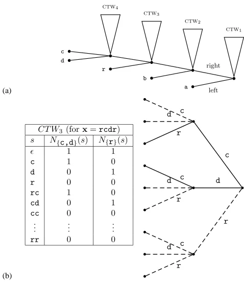
Consider a full binary decomposition tree T with k=_|Σ_|leaves, where each leaf is uniquely associated with a symbol in Σ. Each internal node v of T corresponds to the binary problem of predicting whether the next symbol is a leaf on v’s left subtree or a leaf on v’s right subtree. For ex-ample, forΣ=_{a,b,c,d,r_}, Figure 2 depicts a decomposition tree T such that its root corresponds to the problem of predicting whether the next symbol isaor one of the symbols in_{b,c,d,r_}. The idea is to learn a binary predictor that is based on theCTWalgorithm, for each internal node.

Let v be any internal node of T and letL(v)(resp.,R(v)) be the left (resp., right) child of v. Also, letΣv be the set of leaves (symbols) in the sub-tree rooted by v. We denote by CTWv any perfect

k-ary tree that provides binary predictions over the binary alphabet _{0v,1v}. The supersymbol 0v (resp., 1v) represents any of the symbols inΣL(v) (resp., ΣR(v)). While CTWv generates binary predictions (for its supersymbols), it still depends on a suffix set over the entire k-ary alphabetΣ. Thus, internal node v yields the probability PCTWv(σsuper|s), whereσsuper∈ {0v,1v}and s∈

S

⊆

Σ≤D_{. For example, in Figure 2(b) we depict CTW}

3. Observe that ˆzsestimates a binary distribution that is based on the counts appearing in the table of Figure 2(b).

Let x be any sequence and σ_∈Σ. Algorithm DECO generates the multi-alphabet prediction

PDECO(σ|x)by multiplying the binary predictions of allCTWv along the path from the root of T to the leafσ. Hence, PDECO(σ_|x) =∏v,s.t.,σ_∈ΣvPCTWv(σ|x), where PCTWv(σ|x)is the binary prediction

(a)

ctw1

right ctw2

ctw3

ctw4

c d

r

b

a left

(b)

CT W3(forx=rcdr₎ s N{c,d}(s) N{r}(s)

² 1 1

c 1 0

d 0 1

r 0 0

rc 1 0

cd _{0 1}

cc _{0 0}

..

. ... ...

rr 0 0

c c

d

r

d c

d

r

r

c d

r

Figure 2: ADECOpredictor corresponding to the sequenceabracadabra. (a) depicts the decom-position tree T . Each internal node in T utilizes a CTW predictor to “solve” a binary problem. In (b) we depictCTW₃, a 2-bounded predictor whose binary problem is: “deter-mine ifσ_{∈ {}c,d_}(orσ=r).” (N_σ(s)denotes the frequency ofσinSUBs(x)and dashed lines mark tree paths with zero counts).

There are many possibilities for constructing the decomposition tree T .4 A major open problem is how to identify useful decomposition trees. Intuitively, it appears that placing high frequency symbols close to the root is a good idea for two reasons: (i) When traversing the tree from the root to such symbols, the number of visits to other internal nodes is minimized, thus reducing extra loss; (ii) High frequency symbols appearing closer to the root could be involved in “easier” binary problems because of the denser statistics we have on them.

Tjalkens et al. (1997) and Volf (2002, Chapter 5) suggested taking T as the Huffman coding tree computed with respect to the frequency counts of the symbols in xn₁. While intuitively appealing, there is currently no compelling explanation for this heuristic. In Section 3.1 we provide a formal motivation for Huffman decompositions.

4. We can map every decomposition tree with the partition of 1 into sums of k terms, each of which is a power of 1/2, where each leafσat level`σ defines the power(1/2)`σ_{. (This is possible due to Kraft’s inequality.) Therefore,}

3. Redundancy Bounds For the DECO Algorithm

We start this section with some definitions that formalize the hierarchical alphabet decomposition approach. We also define a new category of sources called “decomposed sources,” which will aid in the analysis of algorithm DECO. To this end, we use an equivalence between decomposed sources and the ordinary tree-sources of Section 2.1. The main result of this section is Theorem 19, providing a pointwise redundancy bound for theDECOalgorithm. This bound, in particular, implies

a performance guarantee for Huffman decomposition trees, which is given in Corollary 23. LetΣbe a multi-alphabet with k symbols and fix some order bound D and initial context x0

1₋D. We refer to a decomposition-tree (see Section 2.4) simply as a tree and to an ordinary tree source as a multi-source, denoted by M= (

S

,PS).

Definition 13 (Decomposed Source) A (D-bounded) decomposed source

T

overΣis a pair

T

= (T,_{M1,M2,_···,Mk₋1}),

where T is a (decomposition) tree overΣand for each internal node, v_∈T , there is a matching source Mv = (

S

v,Pv) whose suffix set,

S

v, contains all paths of some full k-ary tree (of maximal

height D). Additionally, for every s_∈

S

_{v,Pv(·|s)is a binary distribution over{0v,1v}. Note that Miis}

not a standard multi-source because it predicts binary sequences of supersymbols while depending on multi-alphabet contexts. Such sources will always be denoted by Mv for some internal node v.

Let x_∈ΣDbe any sequence andσ_∈Σ. The prediction induced by

T

_is

PT(σ|x) =

∏

v,s.t.,σ_∈Σv

Pv(σ|x). (22)

We say that two probabilistic tree-sources overΣare equivalent if they agree on the probability of every sequence x_∈Σ∗. Note that two structurally different tree-sources can be equivalent. A multi-source is minimal if it has no redundant suffixes. A decomposed source is minimal if all its

Mvmodels are minimal. The formal definitions follow.

Definition 14 (Minimal Sources) (i) A multi-source M= (

S

_,PS)is minimal if there is no s∈Σ<D

for which PS(·|σis) =PS(·|σjs) for all σi 6=σj and bothσis and σjs are in

S

. (ii) We say that

T

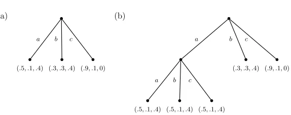
= (T,_{Mv})is a minimal decomposed source if for all internal nodes v of T , Mvis minimal.

For example, we depict in Figure 3 two equivalent multi-sources. The multi-source in Figure 3 (a) is a minimal multi-source while the multi-source in Figure 3 (b) is not minimal.

There is a simple procedure for transforming a non-minimal source into its equivalent minimal form: Replace each redundant suffix,σs, with its suffix s. That is, trim all children of s and assign PS(·|s) =PS(·|σs)for someσ.

The following two lemmas facilitate a “translation” between decomposed and multi sources.

Lemma 15 For every multi-source M and tree T there exists a minimal decomposed source

T

= (T,_{Mv})such that M and

T

are equivalent.

(a)

(.5, .1, .4)

a

(.3, .3, .4)

b

(.9, .1,0)

c

(b)

a

(.5, .1, .4)

a

(.5, .1, .4)

b

(.5, .1, .4)

c

(.3, .3, .4)

b

(.9, .1,0)

c

Figure 3: An example of two equivalent multi-sources. Both sources generate the same probability to every sequence of length larger than two. Take for example x=aaba with initial contextba. Both sources will induce the following prediction: P(aaba_|ba) =0.5·0.5·

0.1_·0.3=0.0075. Observe that the source in (a) is minimal while the other source is not.

∑σ∈0vPS(σ|s)for any (internal node) v and s∈

S

v(=

S

). Similarly, PS(1v|s) =∑σ∈1vPS(σ|s). Let

parent(v)denote the parent of node v. For every internal node v and s_∈

S

_v we define

Pv(0v|s) =PS(0v|s)/Pparent(v)(0v∪1v|s),

and similarly for Pv(1v|s). For the base case (i.e., the root) we do not divide by the denominator. Clearly, Pv(·|s) is a valid distribution and the resulting structure

T

= (T,{Mv}) is a decomposed source.

We shall now prove that

T

_{and M are equivalent. Recall that}

S

₌

S

_{v for every internal node v.} Let v (₆=root) be any internal node in T and u=parent(v). Assume, without loss of generality, that 0v⊂1u, and therefore, 0v∪1v=1u. Note that, for every s∈

S

,

Pu(1u|s)Pv(0v|s) =Pu(1u|s) (PS(0v|s)/Pu(0v∪1v|s)) =PS(0v|s).

Therefore, PT(σ|s) of Equation (22) is a telescopic product; hence, for every σ∈Σ and s∈

S

,

PT(σ|s) =PS(σ|s). This proves that M and

T

are equivalent. Finally, for minimality, we replace

every

S

_vwith its minimal source.

Lemma 16 For every decomposed source

T

there exists a minimal multi-source M that is equiva-lent to

T

.

Proof Let

T

= (T,_{Mv={

S

v,Pv}})be a decomposed source. We provide the following construc-tive scheme for building the equivalent multi-source, M= (

S

,PS). Start with M=Mroot(the model corresponding to the root of T ). We traverse the internal vertices of T (minus the root) such that parent nodes are visited before their descendants (i.e., using preorder). We start with one of the root’s children and for each internal node in T we do the following. For each (internal node) v_∈T

by replacing the supersymbol corresponding to 0v∪1vwith the two (super) symbols 0vand 1v, and define,

PS(0v|s) = PS(0v∪1v|s)·Pv(0v|s);

PS(1v|s) = PS(0v∪1v|s)·Pv(1v|s). (23)

Note that PS(0v∪1v|s)has been already assigned (due to the preorder node traversal). Cases (b) and (c) are treated in exactly the same manner. In case (b) also replace s with its extension sv.

We should now prove that the resulting M= (

S

,PS)is a multi-source and that M is equivalent

to

T

. Both proofs are by induction on_|Σ_|=k. For k=2,

T

consists only of Mroot, which is a binary tree source. Hence, obviously, M=Mroot is a tree source equivalent to

T

. Assume the statement holds for k₋1_≥2 and examine_|Σ_|=k. Let v_∈T be the last visited node in the constructive scheme.

Clearly, by the preorder traversal, the children of v are both leaves (both 0vand 1vare singletons). Merge the two symbols inΣv⊆Σinto some supersymbolσvand consider

T

0= (T0,{Mv0}), which is the decomposed source induced by this replacement. The number of leaves of

T

0_{, which can}

be denoted Σ0=Σ_\Σv∪ {σv}, is equal to k−1. Thus, by the inductive hypothesis, we construct

M0=_{

S

0,PS0}, a multi-source that is equivalent to

T

0. We now apply the constructive step on M0 and v, resulting with M= (

S

,PS). Case (b) of the constructive scheme is the only place that we

change

S

0 (to retrieve

S

).

S

0 is a tree source topology by the induction hypothesis; so is

S

_v and clearly, the treatment of case (b) induces a valid tree-source topology (that corresponds to a full

k-ary tree). Therefore,

S

is a tree-source topology. It is also easy to see that the refinement of the support set of

S

0, as in (23), induces a valid distribution overΣ. We conclude that M= (

S

,PS)is a

multi-source overΣ.

We now turn to prove the equivalence. For every s_∈

S

and any symbolσ_∈Σ_\Σv, we have by Equation (22) that PT(σ|s) =PT0(σ|s), and by the induction hypothesis, PT0(σ|s) =PS0(σ|s). Note that, by the construction, every s0_∈

S

0 is a suffix of some s_∈

S

. Therefore, for symbolsσ_∈Σ_\Σv,

PS0(σ|s0) =PS0(σ|s) =PS(σ|s) (where s0 is the suffix of s). Now for symbolsσ∈Σv, recall that

|Σv|=2 and therefore, 0vrepresents some (ordinary) symbolσ∈Σ(resp., 1v). Thus,

PS(σ|s) = PS0(σ_v|s)P_v(σ|s) (24)

= PT0(σv|s)Pv(σ|s) (25)

=

∏

u, s.t.,u∈T0_∧σ∈Σu

Pu(σ|s)

!

Pv(σ|s) (26)

=

∏

u, s.t.,u∈T∧σ∈Σu

Pu(σ|s) (27)

= PT(σ|s),

where (24) is by the construction (23) withσ_{∈ {}0v,1v}; (25) is by the induction hypothesis; (26) and (27) are by Equation (22). This proves that M is equivalent to

T

. Finally, for satisfying the minimality of M, we take its equivalent minimal multi-source.

Remark 17 It can be shown that a minimal decomposed source (resp., multi-source) is unique.

Consider algorithmDECOapplied with a tree TDECO. The redundancy of theDECOalgorithm on a sequence xn₁, with respect to any decomposed source

T

= (T,_{Mv}), is

RDECO(xn₁,

T

) =log PT(xn₁)−log PDECO(xn₁).

We do not know how to express this redundancy directly in terms of the unknown source

T

_. How-ever, we can express it in terms of an equivalent decomposed source

T

0that has the same tree as in the algorithm. This “translation” is done using an equivalent multi-source mediator that can be con-structed according to Lemmas 15 and 16. To facilitate this discussion, we define, for a decomposed source

T

= (T,_{Mv}), its T0-equivalent source to be any equivalent decomposition source with tree

T0. By Lemmas 15 and 16 this source exists.

Corollary 18 For any decomposed source

T

= (T,_{Mv})and a tree T0there exists a T0-equivalent

source

T

0= (T0,_{M0_i}).

Theorem 19 Let TDECO be any tree and xn1 a sequence. For every internal node v∈TDECO, denote

by CTWv the corresponding CTWpredictor of the DECO algorithm applied with TDECO. Let

T

= (T,_{Mv})be any decomposed source. Then, RDECO(xn1,PT)≤∑

k₋1

i=1Ri(xn1),where i is an internal-node in TDECO, and

Ri(xn1) =

  

 

|S_i|

2 log

ni

|S_i|+|

S

i|+k| S_i|−1

k−1 ,ni≥ |

S

i|; ni+k|

S_i|−1

k−1 ,0<ni<|

S

i|;

0 ,ni=0.

(28)

S

_iis the suffix set of the ith (internal) node of the T0-equivalent source of

T

, and niis the number of

times this node is visited when predicting xn

1.

Proof Let

T

0= (TDECO,{Mv0})be the TDECO-equivalent decomposed source of

T

. Fix any order on the internal nodes of TDECO. We will refer to internal nodes both by their order’s index and by the notation v. By the chain-rule, Pv(xn₁) =∏xt∈ΣvPv(xt|x

t−1

1−D), where Pv(xt|x t−1

1−D) =Pv(xt|s)and s∈

S

v is a suffix of xt₁−₋1_D. Thus,

PT(xn₁) = PT0(xn₁) (29)

= n

∏

t=1

PT0(x_t|xt₁−₋1_D)

= n

∏

t=1v_∈TDECO

∏

, s.t.,xt∈Σv

Pv(xt|xt₁−₋1_D)

=

∏

v∈TDECO

∏

xt∈Σv

Pv(xt|xt₁−₋1_D) =

∏

v∈TDECO

Pv(xn1), (30)

We show that RDECO(xn₁,PT)≤∑_ik₌₁−1Ri(xn1).

RDECO(xn₁,PT) = log PT(xn₁)−log PDECO(xn₁) (31)

= log PT0(xn₁)−log PDECO(xn₁) (32)

= k−1

∑

j=1

log Pj(xn1)−

k−1

∑

i=1

log PCTWi(x n

1) (33)

= k−1

∑

i=1

(log Pi(xn1)−log PCTWi(x n

1)) (34)

≤

k−1

∑

i=1 Ri(xn1),

where (31) follows from Corollary 18; in Equations (32) and (33) the probabilities Pjand Pirefer to internal nodes of

T

0_{; in (32) we used Equation (30); and finally, equality (34) directly follows from}

the proof of Theorem 9. In that proof, we applied the bound (18) for the term (14 i) with k=2, because the zero-order predictors, zs(·) , of CTWv provide binary predictions. The bound on the term (14 ii) remains as is becauseCTWvuses a k-ary tree.

The precise values of the model orders _|

S

_i|in the above upper bound are unknown since the decomposed source is unknown. Nevertheless, for each i, _|

S

_{i| ≤}kD. It follows that any DECO

scheme is universal with respect to the class of D-bounded (multi) tree-sources. Specifically, given any multi-source, consider its TDECO-equivalent decomposed source

T

. For a sequence xn₁, by Theo-rem 19 the per-symbol redundancy is 1_nRDECO(xn₁,PT)≤_n1∑k_i=1−1Ri(xn1), which vanishes with n since ni≤n for every internal-node i.

Remark 20 The dependency of theDECOalgorithm on the maximal bound D and the initial context

x0_1−Dcan be eliminated by using the extensions for theCTWalgorithm suggested by Willems (1998). Recall that Willems provided a point-wise redundancy bound for this case (see Remark 11). Thus, we can straightforwardly use this result to derive a corresponding bound for theDECOalgorithm (the details are omitted).

3.1 Huffman Decompositions

The general bound of Theorem 19 holds for any decomposition tree. However, it is expected that some trees will result in a tighter bound. Therefore, it is desirable to optimize the bound over all trees. Unfortunately, the sizes_|

S

_i|are unknown. Even if the sizes_|

S

_i|were known, it is an NP-hard problem even to decide on the optimal partition corresponding to the root. This hardness result can be obtained by a reduction from MAX-CUT (see, e.g., Papadimitriou, 1994, Chapter 9.3). Hence, we can only hope to approximate the optimal tree.

However, if we replace each_|

S

_i|value with its maximal value kD, we are able to show that the bound is optimized when the decomposition tree is the Huffman decoding tree (see, e.g., Cover and Thomas, 1991, Chapter 5.6) of the sequence xn₁.

For any decomposition tree T and a sequence xn

Lemma 21 Let xn₁be a sequence and T a decomposition tree constructed using Huffman’s proce-dure, which is based on the empirical distribution ˆP(σ) =Nσ/n. Let _{ni} be the counters of T .

Then,∑k_i=1−1niand∏ki=1−1niare both minimal with respect to any other decomposition tree.

Proof Any tree T induces the following prefix-code overΣ. The codeword of a symbolσ∈Σis the path from the root of T to the leafσ. The length of this code for some T , with respect to xn₁, is

`(xn₁) =∑n

t=1`(xt), where`(xt)is the codeword length of the symbol xt. It is not hard to see that

`(xn₁) =

∑

σ Nσ·`(σ) =

k−1

∑

i=1

ni. (35)

If T is constructed using Huffman’s algorithm, the average code length, 1_n∑_σN_σ·`(σ), is the smallest possible. Therefore, T minimizes 1_n∑k_i=1−1ni.

To prove that Huffman’s tree also minimizes ∏k_i=1−1ni, we define the following lexicographic order on the set of inner nodes of any tree. Given a tree, we let nvbe the counter corresponding to inner node v. We can order the inner nodes, first in ascending order of their counters nv, and then (among nodes with equal counters), in ascending order of the heights of the sub-trees they root. Let

T be a Huffman tree, and T0 be any other tree. Let_{nv}be the counters of T and let{nv0}be the counters of T0. We already know that∑vnv≤∑v0nv0. We can order (separately) both sets of counters according to the above lexicographic order such that nv1 ≤ ··· ≤nvk−1 (and similarly, for v0i). We prove, by induction on k, that nvi≤nv0i, for i=1, . . . ,k−1. For k=2 the statement trivially holds.

Assume that for i=1, . . . ,k−1, nvi ≤nv0i. We examine now the case where i=1, . . . ,k. According

to the construction scheme of the Huffman tree (see, Cover and Thomas, 1991, Chapter 5.6), we have that nv1 ≤nv01. Note that the children of v1and v

0

1are all leaves. Otherwise, the non-leaf child

must have the same counter as its parent and is rooting a sub-tree with smaller height. Therefore, by our lexicographic order, the counter of this child must appear before the counter of its parent, which is a contradiction.

Replace v1(resp., v01) with a leaf. Note that every node v (resp., v0) in the resulting trees keeps

its original counter nv (resp., nv0). Hence, nodes can change their order only with nodes of equal counter. Thus, by applying the inductive hypothesis we concluded that nvi ≤nv0i for i=1, . . . ,k.

Remark 22 After establishing Lemma 21, we found that Glassey and Karp (1976) showed that if

f(_·) is an arbitrary concave function, then the Huffman tree minimizes ∑k_i=1−1f(ni). This general

result clearly implies Lemma 21.

From Lemma 21 it follows that the tree constructed by Huffman’s algorithm minimizes any linear function of either∑inior∑ilog ni, which proves, using Theorem 19, the following corollary.

Corollary 23 Let ¯Ri be the Ri of Equation (28) with every|

S

i|replaced by its maximal value, kD.

4. Mind the Gap

Here we compare our redundancy (upper) bound forDECO and the known bound for multi-CTW. Relying on Corollary 23, we focus on the case whereDECOuses the Huffman tree.

A clear advantage of the DECOalgorithm is that it “activates” only internal node (binary)

pre-dictors corresponding to observed symbols. This can be seen by the bound of Theorem 19, which decreases with the number of unobserved symbols. Since the multi-CTWbound is insensitive to al-phabet sparsity, this suggests thatDECOwill outperform the multi-CTWwhen predicting sequences

in which alphabet symbols are sparse.

In this section we prove that the redundancy bound of DECO is strictly better than the corre-sponding multi-CTWbound, for any sufficiently long sequence. For this purpose, we examine the

difference between the two bounds using a worst-case expression of theDECObound.

LetΣbe an alphabet with_|Σ_|=k and xn₁be a sequence overΣ. Fix some order D and let

S

be the topology corresponding to the D-bounded tree-source that maximizes the probability of xn₁over

C

_{D. Denote by ¯RCTW the multi-}CTWredundancy bound (see Theorem 9),

¯

RCTW(xn1) =

(k₋1)_|

S

_|

2 log

n

|

S

_|+|

S

|log k+

k_|

S

_{| −}1

k₋1 . (36)

Similarly, let ¯RHUFFdenote the redundancy ofDECOapplied with a Huffman-tree (see Theorem 19),

¯

RHUFF(xn₁) = k−1

∑

i=1

_Ψ

2 log

ni

Ψ+Ψ+ kΨ₋1

k₋1

, (37)

where Ψ is an upper-bound on the model-sizes _|

S

_i|(see Equation 28). We would like to bound below the gap ¯RCTW−R¯HUFFbetween these bounds.

The next lemma and corollary provide a worst case upper bound for ¯RHUFF.

Lemma 24 Let xn₁be a sequence overΣ. Let T be the corresponding Huffman decomposition tree and_{ni}k_i=1−1its internal node counters. Then,

k₋1

∑

i=1

log ni<(k−1)·(log n+log(1+log k)−log(k−1)) (38)

Proof Recall that for every symbolσ_∈Σ, N_σdenote the number of occurrences ofσin xn₁and`(σ) denotes the length of the path from the root of T to the leafσ. Denote by ˆH the empirical entropy,

ˆ

H=₋∑_σ∈ΣNσ n log

Nσ n.

k−1

∑

i=1

1

k₋1log ni ≤ log k−1

∑

i=1

1

k₋1log ni !

(39)

= log k₋1

∑

i=1

log ni

!

−log(k₋1)

= log

∑

σ∈Σ Nσ`(σ)

!

−log(k₋1) (40)

< log n·(1+_Hˆ_{)−log(k−1) (41)}

≤ log(n_·(1+log k))₋log(k₋1) (42)

In (39) we used Jensen’s inequality; (40) is an application of Equation (35); T yields a Huffman code with an average code length of ∑_σ∈ΣN_nσ`(σ)<1+_{H (see, e.g., Cover and Thomas, 1991,}ˆ Section 5.4 and 5.8), which implies (41); finally, (42) follows from the fact that ˆH_≤log k (see, e.g., Cover and Thomas, 1991, Theorem 2.6.4). We conclude by multiplying both sides by k−1.

Corollary 25

¯

RHUFF(xn₁)<(k−1)Ψ

2

log n

Ψ+log(1+log k)−log(k−1) +2+

2k

k₋1

.

Proof

¯

RHUFF(xn₁) = k₋1

∑

i=1

_Ψ

2 log

ni

Ψ+Ψ+ kΨ₋1

k₋1

= k−1

∑

i=1

_Ψ

2 log ni

+ k−1

∑

i=1

−Ψ₂ log(Ψ) +Ψ+kΨ−1

k₋1

= Ψ

2 k−1

∑

i=1

(log ni) + (k−1)

−Ψ

2 log(Ψ) +Ψ+

kΨ−1

k₋1

< (k−1)Ψ

2 (log n+log(1+log k)−log(k−1)) +

(k₋1)

−Ψ

2 log(Ψ) +Ψ+

kΨ₋1

k−1

(44)

= (k−1)Ψ 2

log_Ψn +log(1+log k)₋log(k−1)+ (k−1)

Ψ+kΨ−1

k₋1

< (k−1)Ψ

2

log n

Ψ+log(1+log k)−log(k−1) +2+

2k

k₋1

. (45)

Here (44) follows by application of (38) and we obtained (45) using k_kΨ₋−₁1<_kk₋Ψ₁.

The next theorem characterizes cases where the DECO algorithm has a strictly smaller redun-dancy bound than the multi-CTWbound.

Theorem 26 LetΣbe an alphabet with_|Σ_|=k_≥118 and xn₁ be a sequence overΣgenerated by the (unknown) D-bounded multi-source

M

= (

S

,PS). Then, ¯RCTW(xn₁)>R¯HUFF(xn₁).

be pruned to achieve minimality. Hence,|

S

_{|is an upper bound on the sizes|}

S

_{i|. Thus, we have}

¯

RCTW(xn₁)_−R¯_HUFF(xn

1) =

(k₋1)_|

S

_|

2 log

n

|

S

_|+|

S

|log k+

k_|

S

_{| −}1

k₋1 − k−1

∑

i=1

|

S

_| 2 log

ni

|

S

_|+|

S

|+

k_|

S

_{| −}1

k₋1

> (k−1)|

S

|

2 log

n

|

S

_|+|

S

|log k+

k_|

S

_{| −}1

k−1 −

(k₋1)_|

S

_|

2 ×

log n

|

S

_|+log(1+log k)−log(k−1) +2+ 2k

k−1

(46)

= _|

S

_|log k+k|

S

| −1

k₋1 − (k₋1)_|

S

_|

2

log(1+log k)₋log(k₋1) +2+ 2k

k₋1

, (47)

where (46) is by Corollary 25. Using straightforward analysis it is not hard to show that (47) grows with k and is positive for k_≥118. This completes the proof.

The gap, between theCTWandDECObounds, shown in Theorem 26 is relevant when the inter-nal node redundancies of DECOare Ri= |

S_i|

2 log

ni

|Si|+|

S

i|+ k|S_i|−1

k₋1 . By a simple analysis of

Equa-tion (28) using the funcEqua-tion f(x) = x₂logn_x+x+kx_k−−₁1, we can show that the gap is positive when

ni≥max{0.17·Ψ,

S

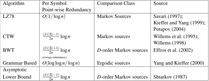
i}.

We conclude that the redundancy bound ofDECOalgorithm converges faster than the bound of the CTWalgorithm for alphabet of size k_≥118. Currently, theCTWalgorithm is known to have the best convergence rate (see Table 5). Therefore, the current bound is the tightest one known for prediction (and lossless compression) in realistic settings.

Remark 27 The result of Theorem 26 is obtained using a worst-case analysis for the DECO re-dundancy. This analysis considered a sequence that contains all alphabet symbols; each symbol appears sufficiently many times. However, in many practical applications (such as predictions of ASCII sequences) most of the symbols are expected to have small frequencies (e.g., by Zipf ’s Law). In this case, the DECOredundancy is even smaller than the worst case bound of Corollary 25 and the gap between the two bounds is larger.

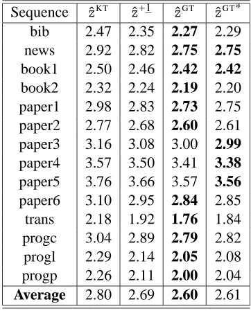
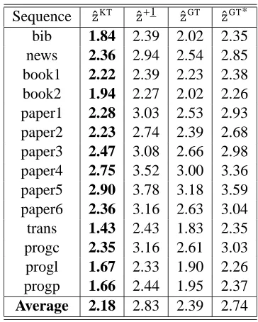
5. Examining Other Alphabet Decompositions

The bound ¯RHUFF, given in Equation (37), is optimized using a Huffman decomposition tree (Corol-lary 23). However, replacing each _|

S

_i|with its maximal value can affect the bound considerably. For example, if we manage to place a very easy (binary) prediction problem at the root, it could be the case that the “true” model order for this problem is very small. Such considerations are not explicitly treated by the Huffman tree optimization. Therefore, it is of major interest to consider other types of alphabet decomposition trees. Also, if our goal is to utilize the (successful) binary

CTW in multi-alphabet problems, there is no apparent reason why we should restrict ourselves to

de-compositions” in supervised learning suggests other approaches such one-vs-all, all-pairs, etc. (see, e.g., Allwein et al., 2001).

We empirically targeted two questions: (i) Are there better alphabet decomposition trees for the

DECOalgorithm? (ii) Can the “flat” decomposition techniques of supervised learning be effectively applied in our sequential prediction setting?

To answer the first question, we developed a simple heuristic procedure that attempts to increase log-likelihood performance of the DECO algorithm, starting from any decomposition tree. This

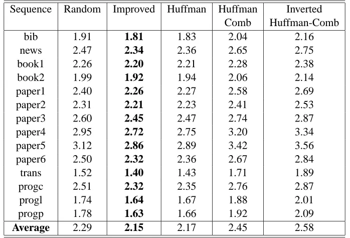
procedure searches for a locally optimal tree using the actual performance of DECO on a given sequence. Starting from a given tree, this procedure attempts to swap an alphabet symbol from one subtree to the other while recursively “optimizing” the resulting subtrees. Each such swap is ‘accepted’ only if it improves the actual performance. We applied this procedure using a Huffman tree as the starting point and refer to the resulting algorithm as ‘Improved’.

Sequence Random Improved Huffman Huffman Inverted

Comb Huffman-Comb

bib 1.91 1.81 1.83 2.04 2.16

news 2.47 2.34 2.36 2.65 2.75

book1 2.26 2.20 2.21 2.28 2.38

book2 1.99 1.92 1.94 2.06 2.14

paper1 2.40 2.26 2.27 2.58 2.69

paper2 2.31 2.21 2.23 2.41 2.53

paper3 2.60 2.45 2.47 2.74 2.87

paper4 2.95 2.72 2.75 3.20 3.34

paper5 3.12 2.86 2.89 3.42 3.56

paper6 2.50 2.32 2.36 2.67 2.84

trans 1.52 1.40 1.43 1.71 1.89

progc 2.51 2.32 2.35 2.76 2.87

progl 1.74 1.64 1.67 1.88 2.01

progp 1.78 1.63 1.66 1.92 2.09

Average 2.29 2.15 2.17 2.45 2.58

Table 1: Comparing average log-loss ofDECO with different decomposition structures. The best results appear in boldface. Results for the random decomposition reflect an average on ten random trees.