Joint Estimation of Multiple Precision Matrices
with Common Structures
Wonyul Lee [email protected]
Department of Statistics and Operations Research University of North Carolina
Chapel Hill, NC 27599-3260, USA
Yufeng Liu [email protected]
Department of Statistics and Operations Research Department of Genetics
Department of Biostatistics
Carolina Center for Genome Sciences University of North Carolina
Chapel Hill, NC 27599-3260, USA
Editor:Francis Bach
Abstract
Estimation of inverse covariance matrices, known as precision matrices, is important in various areas of statistical analysis. In this article, we consider estimation of multiple precision matrices sharing some common structures. In this setting, estimating each preci-sion matrix separately can be suboptimal as it ignores potential common structures. This article proposes a new approach to parameterize each precision matrix as a sum of com-mon and unique components and estimate multiple precision matrices in a constrainedl1 minimization framework. We establish both estimation and selection consistency of the proposed estimator in the high dimensional setting. The proposed estimator achieves a faster convergence rate for the common structure in certain cases. Our numerical examples demonstrate that our new estimator can perform better than several existing methods in terms of the entropy loss and Frobenius loss. An application to a glioblastoma cancer data set reveals some interesting gene networks across multiple cancer subtypes.
Keywords: covariance matrix, graphical model, high dimension, joint estimation, preci-sion matrix
1. Introduction
dimension p is comparable to or much larger than the sample size n, more feasible and stable techniques are required for accurate estimation of a precision matrix.
To tackle such problems, various penalized maximum likelihood methods have been considered by many researchers in recent years (Yuan and Lin, 2007; Banerjee et al., 2008; Friedman et al., 2008; Rothman et al., 2008; Lam and Fan, 2009; Fan et al., 2009, and many more). These approaches produce a sparse estimator of the precision matrix by maximizing the penalized Gaussian likelihood with sparse penalties such as the l1 penalty and the smoothly clipped absolute deviation penalty (Fan and Li, 2001). Ravikumar et al. (2011) studied the theoretical properties of the l1 penalized likelihood estimator for a broad class of population distributions.
Instead of using likelihood approaches, several techniques take advantage of the con-nection between linear regression and the entries of the precision matrix. See for example Meinshausen and B¨uhlmann (2006); Peng et al. (2009); Yuan (2010). In particular, these approaches convert the estimation problem of the precision matrix into relevant regression problems and solve them with sparse regression techniques accordingly. One advantage of these approaches is that they can handle a wide range of distributions including the Gaus-sian case. Cai et al. (2011) recently proposed a very interesting method to directly estimate the precision matrix without the Gaussian distributional assumption. This approach solves a constrained l1 minimization problem to obtain a sparse estimator of the precision ma-trix. They showed that the proposed estimator has a faster convergence rate than the l1 penalized likelihood estimator for some non-Gaussian cases.
All aforementioned approaches focus on estimation of a single precision matrix. The fundamental assumption of these approaches is that all observations follow the same dis-tribution. However, in some real applications, this assumption can be unreasonable. As a motivating example, consider the glioblastoma multiforme (GBM) cancer data set studied by The Cancer Genome Atlas Research Network (The Cancer Genome Atlas Research Net-work, 2008). It is shown in the literature that the GBM cancer can be classified into four subtypes (Verhaak et al., 2010). In this case, it would be more realistic to assume that the distribution of gene expression levels can vary from one subtype to another, which results in multiple precision matrices to estimate (Lee et al., 2012). A naive way to estimate them is to model each subtype separately. However, in this separate approach, modeling of one subtype completely ignores the information on other subtypes. This can be suboptimal if there exists some common structure across different subtypes.
To improve the estimation in presence of some common structure, several joint esti-mation methods have been proposed recently in a penalized likelihood framework. See for example Guo et al. (2011); Honorio and Samaras (2012); Danaher et al. (2014). These methods employ various group penalties in the Gaussian likelihood framework to link the estimation of separate precision matrices.
if the precision matrices are similar to each other. Furthermore, our method is able to discover unique structures of each precision matrix, which enables us to identify differences among multiple precision matrices. The proposed estimator is shown to achieve a faster convergence rate for the common structures in certain cases.
The rest of this article is organized as follows. In Section 2, we introduce our proposed method after reviewing some existing separate approaches. We establish its theoretical properties in Section 3. Section 4 develops computational algorithms to obtain a solution for the proposed method. Simulated examples are presented in Section 5 to demonstrate performance of our estimator and analysis of a glioblastoma cancer data example is provided in Section 6. The proofs of theorems are provided in Appendix.
2. Methodology
In this section, we introduce a new method for estimating multiple precision matrices in an l1 minimization framework. Consider a heterogeneous data set withG different groups. For the gth group (g = 1, . . . , G), let {x(g)
1 , . . . , x (g)
ng} be an independent and identically
distributed random sample of size ng, where x(g)k = (x(g)ki, . . . , x(g)kp)T is a p-dimensional
ran-dom vector with the covariance matrix Σ(g)
0 and precision matrix Ω (g)
0 := (Σ (g)
0 )−1. For detailed illustration of our proposed method, we first define some notations similar to Cai et al. (2011). For a matrix X = (xij) ∈ Rp×q, we define the elementwise l1 norm
||X||1 = Pp
i=1
Pq
j=1|xij|, the elementwise l∞ norm |X|∞ = max1≤i≤p,1≤j≤q|xij| and the
matrix l1 norm ||X||L1 = max1≤j≤qPpi=1|xij|. For a vector x = (x1, . . . , xp)T ∈ Rp, |x|1 and |x|∞ denote vector l1 and l∞ norms respectively. The notation X 0 indicates that
X is positive definite. LetI be ap×p identity matrix. For thegth group, ˆΣ(g) denotes the sample covariance matrix. Write Ω(g)0 = (ω(g)ij,0);g= 1, . . . , G.
Our aim is to estimate the precision matrices, Ω(1)0 , . . . ,Ω(G)0 . The most naive way to achieve this goal is to estimate each precision matrix separately by taking the inverses of the sample covariance matrices. However, in high dimensional cases, the sample covari-ance matrices are not only unstable for estimating the covaricovari-ance matrices, but also not invertible. To estimate the precision matrix in high dimensions, various estimators have been introduced in the literature. For example, various l1 penalized Gaussian likelihood estimators have been studied intensively in the literature (see for example, Yuan and Lin, 2007; Banerjee et al., 2008; Friedman et al., 2008; Rothman et al., 2008). In this framework, the precision matrices can be estimated by solving the followingGoptimization problems:
min Ω(g)0tr( ˆΣ
(g)Ω(g))−log{det(Ω(g))}+λ g
X
i6=j
|w(g)
ij |, g= 1, . . . , G, (1)
where λg is a tuning parameter which controls the degree of the sparsity in the estimated
precision matrices. Other sparse penalized Gaussian likelihood estimators have been pro-posed as well (Lam and Fan, 2009; Fan et al., 2009).
optimization problem:
min||Ω(g)||
1 subject to: |Σˆ (g)
Ω(g)−
I|∞≤λg, (2)
where ˆΣ(g)is the sample covariance matrix andλ
gis a tuning parameter. As the optimization
problem in (2) does not require symmetry of the solution, the final CLIME estimator is obtained by symmetrizing the solution of (2). The CLIME estimator does not need the Gaussian distributional assumption. Cai et al. (2011) showed that the convergence rate of the CLIME estimator is faster than that of the l1 penalized Gaussian likelihood estimator if the underlying true distribution has polynomial-type tails.
To estimate multiple precision matrices, Ω(1) 0 , . . . ,Ω
(G)
0 , we can buildGindividual models using the optimization problem (1) or (2). However, these separate approaches can be suboptimal when the precision matrices share some common structure. Several recent papers have proposed joint estimations of multiple precision matrices under the Gaussian distributional assumption to improve estimation. In particular, such an estimator is the solution of
min {Ω}
G
X
g=1
ng
h
tr( ˆΣ(g)Ω(g))−log{det(Ω(g))}i+P({Ω}),
where ng is the sample size of the g-th group, {Ω} = {Ω(1), . . . ,Ω(G)}, and P({Ω}) is
a penalty function that encourages similarity across the G estimated precision matrices. For example, Guo et al. (2011) employs a non-convex penalty called hierarchical group penalty which has the form, P({Ω}) = λP
i6=j
PG
g=1|ω (g) ij |
1/2
. Honorio and Samaras
(2012) adopts a convex penalty, P({Ω}) = λP
i6=j|(ω (1) ij , . . . , ω
(G)
ij )|p (p > 1) where | · |p is
the vector lp norm. To separately control the sparsity level and the extent of similarity,
Danaher et al. (2014) considered a fused lasso penalty, P({Ω}) = λ1PGg=1
P
i6=j|ω (g) ij |+
λ2Pg<g0
P
ij|ω (g) ij −ω
(g0)
ij |. In some simulation settings, they showed that the joint estimation
can perform better than separatel1 penalized normal likelihood estimation. As pointed by Ravikumar et al. (2011), these penalized Gaussian likelihood estimators are applicable even for some mild non-Gaussian data since maximizing a penalized likelihood can be interpreted as minimizing a penalized log-determinant Bregman divergence. However, these approaches were mainly designed for Gaussian data and can be less efficient when the underlying distribution becomes far from Gaussian. In this paper, we propose a new joint method for estimating multiple precision matrices, which is less dependent on the distributional assumption and applicable for both Gaussian and non-Gaussian cases.
In our joint estimation method, we take the multi-task learning perspective and first define the common structureM0 and the unique structureR(g)0 as
M0 := 1
G
G
X
g=1
Ω(g)0 , R0(g):= Ω(g)0 −M0;g= 1, . . . , G.
It follows from the definition that PG
g=1R (g)
was previously considered in the context of supervised multi-tasking learning (Evgeniou and Pontil, 2004). Their aim was to improve prediction performance of supervised multi-tasking learning. Here we focus on better estimation of precision matrices with the common and individual structures. The unique structure is defined to capture different strength of the edges across all classes. In a special case that an element of M0 is zero, then the corresponding nonzero element in R(g)0 can be interpreted as a unique edge. Thus, the unique structure can address differences in magnitude as well as unique edges. If all precision matrices are very similar, then the unique structures defined above would be close to zero. In this case, it can be natural and advantageous to encourage sparsity among{R(1)0 , . . . , R(G)0 }
in the estimation. To estimate the precision matrices consistently in high dimensions, it is also necessary to assume some special structure ofM0 as well. In our work, we also assume that M0 is sparse. To estimate {M0, R(1)0 , . . . , R(G)0 }, we propose the following constrained
l1 minimization criterion:
min{||M||1+ν
G
X
g=1
||R(g)|| 1}
s.t |1
G
G
X
g=1
{Σˆ(g)
(M+R(g)
)−I}|∞≤λ1,|Σˆ(g)(M+R(g))−I|∞≤λ2, G
X
g=1
R(g)
= 0, (3)
whereλ1 andλ2 are tuning parameters andνis a prespecified weight. Note that ifλ1 > λ2, then the second inequality constraints in (3) imply the first inequality constraint. Therefore, we only consider a pair of (λ1, λ2) satisfying λ1≤λ2. The first inequality constraint in (3) reflects how close the final estimators are to the inverses of the sample covariance matrices in an average sense. On the other hand, the second inequality constraint controls an individual level of closeness between the estimators and the sample covariance matrices.
For illustration, consider an extreme case where all the precision matrices are the same. In this case, the unique structures may be negligible and the first inequality constraint in (3) approximately reduces to|(G−1PG
g=1Σˆ
(g))M−I|
∞≤λ1. Therefore, we can pool all the sample covariance matrices to estimate the common structure which is the precision matrix in this case. This would be advantageous than building each model separately. The value ofν in (3) reflects how complex the unique structures of the resulting estimators are. If the resulting estimators are expected to be very similar from each other, then a large value of
ν is preferred. In Section 3,ν is set to beG−1 orG−1/2 for our theoretical results.
Similar to Cai et al. (2011), the solutions in (3) are not symmetric in general. Therefore, the final estimators are obtained after a symmetrization step. Let {M ,ˆ Rˆ(1), . . . ,Rˆ(G)} be the solution of (3). Then we define ˆΩ(g)
1 := ˆM + ˆR(g);g = 1, . . . , G. The final estimator of
{Ω(1)0 , . . . ,Ω(G)0 } is obtained by symmetrizing{Ωˆ(1)1 , . . . ,Ωˆ(G)1 } as follows. Let ˆΩ(g)1 = (ˆωij,(g)1). Our joint estimator of multiple precision matrices (JEMP), {Ωˆ(1), . . . ,Ωˆ(G)}, is defined as symmetric matrices, {Ωˆ(g)= (ˆω(g)
ij );g= 1, . . . , G}with
ˆ
ωij(g)= ˆω(g)ij,1I{
G
X
g=1
|ωˆ(g)ij,1| ≤
G
X
g=1
|ωˆji,(g)1|}+ ˆω(g)ji,1I{
G
X
g=1
|ωˆij,(g)1|>
G
X
g=1
|ωˆ(g)ji,1|};g= 1, . . . , G.
In our simulation study, we observed that within a reasonable range of tuning parameters, almost all solutions are positive definite. Furthermore, one can perform projection of the estimator to the space of positive definite matrices to ensure positive definitiveness as dis-cussed in Yuan (2010).
As a remark, although we focus on generalizing CLIME for multiple graph estimation in this paper, our proposed common and unique structure approach can also be applied to the graphical lasso estimator under the Gaussian assumption as pointed out by one reviewer. As a future research direction, it would be interesting to investigate how the common and unique structure framework works in the graphical lasso estimator.
3. Theoretical Properties
In this section, we investigate theoretical properties of our proposed joint estimator JEMP. In particular, we first construct the convergence rate of our estimator in the high dimensional setting. Then we show that the convergence rate can be improved for the common structure of the precision matrices in certain cases. Finally, the model selection consistency is shown with an additional thresholding step.
For theoretical properties, we follow the set-up of Cai et al. (2011) and the results therein are also used for our technical derivations. In this section, for simplicity, we assume that
n=n1 =· · ·=nG. We consider the following class of matrices,
U :={Ω : Ω0,kΩkL
1 ≤CM},
and assume that Ω(g)0 ∈ U for all g = 1, . . . , G. This assumption requires that the true precision matrices are sparse in terms of thel1norm while allowing them to have many small entries. WriteE(x(g)) = (µ(g)
1 , . . . , µ (g)
p )T. We also make the following moment condition on
x(g) for our theoretical results.
Condition 1 There exists some 0 < η <1/4 such that E[exp{t(x(g)i −µ(g)i )2}]≤K < ∞
for all |t| ≤η and all i, g and Glogp/n≤η, where K is a bounded constant.
Condition 1 indicates that the components of x(g) are uniformly sub-Gaussian. This condition is satisfied if x(g) follows a multivariate Gaussian distribution or has uniformly bounded components.
Theorem 1 Assume Condition 1 holds. Let λ1 = λ2 = 3CMC0(logp/n)1/2, where C0 = 2η−2(2 +τ +η−1e2K2)2 and τ >0. Set ν=G−1. Then
max
ij
1
G
G
X
g=1
|ωˆ(g) ij −ω
(g) ij,0|
≤6CM2 C0
logp n
1/2 ,
with probability greater than 1−4Gp−τ.
Theorem 2 Assume Condition 1 holds. Suppose that there exists CR > 0 such that
kR(g)0 kL1 ≤CR for allg = 1, . . . , G and(
PG
g=1kR (g)
0 kL1)≤CRG
1/2. Set ν =G−1/2 and let
λ1= (CM+CR)C0{logp/(nG)}1/2 andλ2 =CMC0(logp/n)1/2. Then
|Mˆ −M0|∞≤C0(2CM2 + 4CMCR+CR2)
logp nG
1/2 ,
with probability greater than 1−2(1 + 3G)p−τ.
Theorem 2 states that our proposed method can estimate the common part more ef-ficiently with the corresponding convergence rate of order {logp/(nG)}1/2, which is faster than the order (logp/n)1/2.
Note that our theorems show consistency of our estimator in terms of the elementwise
l∞norm. On the other hand, Guo et al. (2011) showed consistency of their estimator under the Frobenious norm. Therefore, our theoretical results are not directly comparable to the theorems in Guo et al. (2011). However, it is worthwhile to note that our Theorem 2 reveals the effect of G on the consistency while the theorems in Guo et al. (2011) do not show explicitly how their estimator can have advantage over separate estimation in terms of consistency.
Besides its estimation consistency, we also prove the model selection consistency of our estimator which means that it reveals the exact set of nonzero components in the true precision matrices with high probability. For this result, a thresholding step is introduced. In particular, a threshold estimator ˜Ω(g)= (˜ω(g)
ij ) based on {Ωˆ
(1), . . . ,Ωˆ(G)} is defined as,
˜
ωij(g) = ˆωij(g)I{|ωˆij(g)| ≥δn},
whereδn≥2CMGλ2 andλ2is given in Theorem 1. To state the model selection consistency precisely, we define
S0 :={(i, j, g) :ω(g)
ij,06= 0},Sˆ:={(i, j, g) : ˜ω (g)
ij 6= 0} and θmin := min (i,j,g)∈S0
G
X
g=1
|ω(g) ij,0|. Then the next theorem states the model selection consistency of our estimator.
Theorem 3 Assume Condition 1 holds. If θmin>2δn, then pr(S0= ˆS)≥1−4Gp−τ. 4. Numerical Algorithm
4.1 Decomposition of (3)
Similar to the Lemma 1 in Cai et al. (2011), one can show that the optimization problem (3) can be decomposed into p individual minimization problems. In particular, let ei be
the ith column of I. For 1≤i≤ p, let {mˆi,ˆr (1) i , . . . ,ˆr
(G)
i } be the solution of the following
optimization problem:
min{|m|1+ν
G
X
g=1
|r(g)| 1}
s.t. |1
G
G
X
g=1
{Σˆ(g)
(m+r(g)
)−ei}|∞≤λ1,|Σˆ(g)(m+r(g))−ei|∞≤λ2, G
X
g=1
r(g)
= 0, (4)
wherem,r(1), . . . , r(G)are vectors inRp. We can show that solving the optimization problem
(3) is equivalent to solving thepoptimization problems in (4). The optimization problem in (4) can be further reformulated as a linear programming problem and the simplex method is used to solve this problem (Boyd and Vandenberghe, 2004). For our simulation study and the GBM data analysis, we obtain the solution of (3) using the efficient R-package fastclime, which provides a generic fast linear programming solver (Pang et al., 2014).
4.2 An ADMM Algorithm
In this section, we describe an alternating directions method of multipliers (ADMM) al-gorithm to solve (4) which can be potentially more scalable than the previously explained linear programming approach. We refer the reader to Boyd et al. (2010) for detailed expla-nation of ADMM algorithms and their convergence properties.
To reformulate (4) into an appropriate ADMM form, definey= (mT, νr(1)T, . . . , νr(G)T)T,
zm=PGg=1{Σˆ
(g)(m+r(g))−e
i}/G,zg = ˆΣ(g)(m+r(g))−ei, and z= (z1T, . . . , zGT, zmT)T.
Denote the a×a identity matrix as Ia×a and the a×b zero matrix as Oa×b. Then the
problem (4) can be rewritten as
min|y|1 s.t. |zm|∞≤λ1,|zg|∞≤λ2, Ay−Bz=C, where (5)
A=
ˆ
Σ(1) ν−1Σˆ(1) O
p×p · · · Op×p
ˆ
Σ(2) O
p×p ν−1Σˆ(2) · · · Op×p
..
. ... ... . .. ...
ˆ
Σ(G) O
p×p Op×p · · · ν−1Σˆ(G)
G−1PG
g=1Σˆ
(g) (νG)−1Σˆ(1) (νG)−1Σˆ(2) · · · (νG)−1Σˆ(G)
Op×p Ip×p Ip×p · · · Ip×p
,
B =
I(1+G)p×(1+G)p
Op×(1+G)p
, and C = (eiT, . . . , eiT, Op×1)T. The scaled augmented Lagrangian for (5) is given by
L(y, z, u) =|y|1+ρ
2||Ay−Bz−C+u|| 2
2, s.t. |zm|∞≤λ1,|zg|∞≤λ2,
(a) yk+1 = argminyL(y, zk, uk).
(b) zk+1 = argminzL(yk+1, z, uk), s.t. |zm|∞≤λ1,|zg|∞≤λ2. (c) uk+1 =uk+Ayk+1−Bzk+1−c.
As argminyL(y, zk, uk) = argminy{|y|1 + ρ2||Ay−Bzk−C+uk||22}, the step (a) can be viewed as anL1penalized least squares problem. Therefore, the step (a) can be solved using some existing algorithms forL1 penalized least squares problems. In addition, one can show that the step (b) has a closed form of solution,zk+1= min{max{A0yk+1−C0+(uk)0,−λ}, λ}
where A0 is the submatrix of A consisting of the first (1 +G)p rows, C0 and (uk)0 are the corresponding subvectors ofC anduk, and λis a (1 +G)p-dimensional vector of which the firstGpelements areλ2 and the rest areλ1. Note that scalability and computational speed of this ADMM algorithm largely depend on the algorithm used for the step (a) as the other steps have the explicit form of solutions.
4.3 Tuning Parameter Selection
To apply our method, we need to choose the tuning parameters, λ1 and λ2. In practice, we construct several models with many pairs of λ1 and λ2 satisfying λ1 ≤λ2 and evaluate them to determine the optimal pair. To evaluate each estimator, we measure the likelihood loss (LL) used in Cai et al. (2011) and its definition is
LL =
G
X
g=1 tr( ˆΣ(g)
v Ωˆ(g))−log{det( ˆΩ(g))},
where ˆΣ(g)v is the sample covariance matrix of thegth group computed from an independent
validation set. As mentioned in Section 2, the likelihood loss can be applicable for both Gaussian and some non-Gaussian data as it corresponds to the log-determinant Bregman divergence between the estimators and empirical precision matrices in the validation set. Among several pairs of tuning values, we select the pair which minimizes LL. If a validation set is not available, aK-fold cross-validation can be combined to this criterion. In particular, we first randomly split the data set intoK parts of equal sizes. Denote the data in thekth part by {X(1)
(k), . . . , X (G)
(k)} which is used as a validation set for thekth estimator. For each
k, with a given value of (λ1, λ2), we obtain estimators using all observations which do not belong to {X(1)
(k), . . . , X (G)
(k)} and denote them as {Ωˆ (G) (k), . . . ,Ωˆ
(G)
(k)}. Then the likelihood loss (LL) is defined as
LL =
K
X
k=1 G
X
g=1 tr( ˆΣ(g)
(k)Ωˆ (g)
(k))−log{det( ˆΩ (g) (k))},
where ˆΣ(g)
(k) is the sample covariance matrix of the gth group usingX (g)
5. Simulated Examples
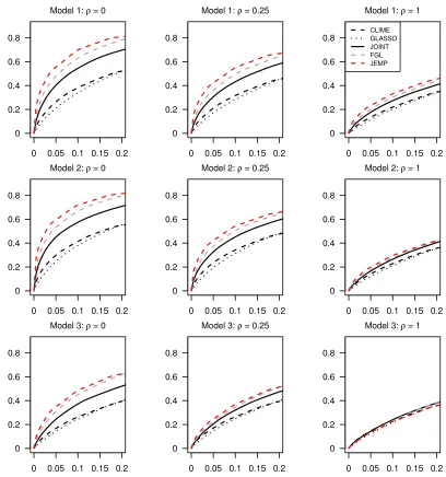
In this section, we carry out simulation studies to assess the numerical performance of our proposed method. In particular, we compare the numerical performance of five methods: two separate methods and three joint methods. In separate approaches, each precision matrix is estimated separately via the CLIME estimator or the GLASSO estimator. For joint approaches, all precision matrices are estimated together using our JEMP estimator, the fused graphical lasso (FGL) estimator by Danaher et al. (2014), or the estimator by Guo et al. (2011), which we refer to as JOINT estimator hereafter. In our proposed method,ν is set to beG−1/2. We also tried different values ofν such asG−1, and the results are similar thus omitted. We consider three models as described below: the first two from Guo et al. (2011) and the last from Rothman et al. (2008); Cai et al. (2011). In all models, we set
p= 100,G= 3 and Ω(g)0 = Ωc+U(g), where Ωcis common in all groups andU(g) represents
unique structure to the gth group. The common part, Ωc, is generated as follows:
Model 1. Ωc is a tridiagonal precision matrix. In particular, Σc:= Ω−c1 = (σij) is first
constructed, whereσij = exp(−|di−dj|/2), d1 < . . . < dp, and di−di−1 ∼Unif(0.5,1), i= 2, . . . , p. Then let Ωc= Σ−c1.
Model 2. Ωc is a 3 nearest-neighbor network. In particular, p points are randomly
picked on a unit square and all pairwise distances among the points are calculated. Then we find 3 nearest neighbors for each point and a pair of symmetric entries in Ωccorresponding
to a pair of neighbors has a value randomly chosen from the interval [−1,−0.5]∪[0.5,1].
Model 3. Ωc = Γ +δI, where each off-diagonal entry in Γ is generated independently
from 0.5y, with y following the Bernoulli distribution with success probability 0.02. Here,
δ is selected so that the condition number of Ωc is equal to p.
For eachU(g), we randomly pick a pair of symmetric off-diagonal entries and replace them with values randomly chosen from the interval [−1,−0.5]∪[0.5,1]. We repeat this procedure until P
i<jI(|u (g)
ij | > 0)/
P
i<jI(|ωij,c| > 0) = ρ, where Ωc = (ωij,c) and U
(g) = u(g) ij.
Therefore,ρ is the ratio of the number of unique nonzero entries to the number of common nonzero entries. We consider four values of ρ = 0,0.25,1 and 4. To make the resulting precision matrices positive-definite, each diagonal element of each matrix Ω(g)0 is replaced with 1.5 times the sum of the absolute values of the corresponding row. Finally, each matrix Ω(g)
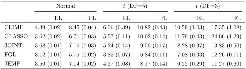
0 is standardized to have unit diagonals. Note that in the case of ρ = 1 or 4, the true precision matrices are quite different from each other. From these cases, we can assess how joint methods work when the precision matrices are not similar. In addition, we also consider Model 4 below to assess how JEMP works when the precision matrices have different structures from each other.
Model 4. Ω(1)
0 is the tridiagonal precision matrix as in Model 1, Ω (2)
0 is the 3 nearest-neighbor network in Model 2, and Ω(3)0 is the random network in Model 3.
ρ= 0 ρ= 0.25
EL FL EL FL
Normal
CLIME 4.42 (0.02) 8.57 (0.03) 4.35 (0.02) 8.42 (0.03)
GLASSO 3.70 (0.02) 6.90 (0.03) 3.60 (0.02) 6.73 (0.03)
JOINT 3.43 (0.02) 6.64 (0.04) 3.41 (0.02) 6.61 (0.03)
FGL 1.99 (0.02) 3.75 (0.03) 2.09 (0.02) 3.92 (0.03)
JEMP 2.08 (0.02) 4.06 (0.04) 2.20 (0.02) 4.31 (0.04)
t(DF=5)
CLIME 5.75 (0.17) 10.63 (0.26) 5.81 (0.19) 10.75 (0.33)
GLASSO 5.60 (0.09) 10.23 (0.16) 5.45 (0.09) 10.00 (0.16)
JOINT 5.08 (0.11) 9.44 (0.15) 5.01 (0.12) 9.28 (0.19)
FGL 3.47 (0.07) 6.12 (0.11) 3.46 (0.08) 6.12 (0.11)
JEMP 3.21 (0.06) 6.14 (0.11) 3.41 (0.10) 6.52 (0.19)
t(DF=3)
CLIME 10.34 (0.83) 18.08 (1.05) 10.15 (0.91) 17.25 (1.06)
GLASSO 11.87 (0.33) 24.10 (0.95) 11.78 (0.33) 24.21 (0.95)
JOINT 8.84 (0.58) 15.16 (0.85) 8.95 (0.66) 15.17 (0.92)
FGL 7.01 (0.24) 12.39 (0.52) 7.40 (0.31) 13.23 (0.66)
JEMP 6.02 (0.33) 11.56 (0.73) 5.95 (0.30) 11.16 (0.62)
ρ= 1 ρ= 4
EL FL EL FL
Normal
CLIME 4.23 (0.02) 8.15 (0.03) 3.67 (0.01) 6.95 (0.03)
GLASSO 3.37 (0.02) 6.33 (0.03) 2.57 (0.01) 4.96 (0.03)
JOINT 3.27 (0.01) 6.40 (0.03) 2.51 (0.01) 4.95 (0.02)
FGL 2.18 (0.01) 4.07 (0.02) 1.82 (0.01) 3.47 (0.02)
JEMP 2.38 (0.01) 4.77 (0.04) 2.11 (0.01) 4.28 (0.02)
t(DF=5)
CLIME 5.53 (0.16) 10.12 (0.23) 4.83 (0.17) 8.72 (0.25)
GLASSO 5.11 (0.09) 9.54 (0.17) 4.28 (0.09) 8.35 (0.19)
JOINT 4.71 (0.10) 8.71 (0.14) 3.87 (0.12) 7.03 (0.16)
FGL 3.31 (0.07) 5.95 (0.11) 2.54 (0.06) 4.68 (0.10)
JEMP 3.32 (0.07) 6.40 (0.13) 2.78 (0.07) 5.35 (0.12)
t(DF=3)
CLIME 9.89 (0.86) 17.82 (1.16) 8.93 (0.91) 16.58 (1.28)
GLASSO 11.32 (0.32) 23.77 (0.99) 10.42 (0.31) 23.70 (1.05)
JOINT 9.27 (1.68) 14.23 (1.26) 7.14 (0.65) 11.90 (0.72)
FGL 6.51 (0.25) 11.73 (0.56) 5.95 (0.27) 11.55 (0.67)
JEMP 5.71 (0.29) 10.99 (0.73) 4.72 (0.24) 9.04 (0.49)
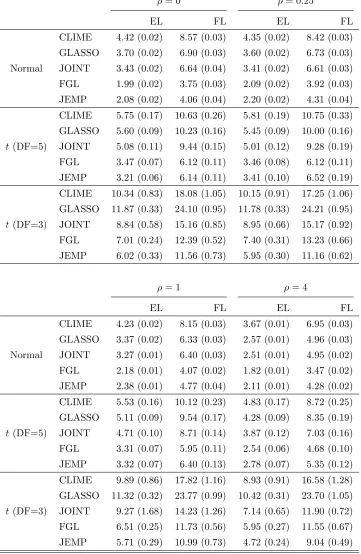
Table 1: Comparison summaries using Entropy loss (EL) and Frobenius loss (FL) over 50
ρ= 0 ρ= 0.25
EL FL EL FL
Normal
CLIME 5.10 (0.02) 9.80 (0.04) 5.05 (0.02) 9.68 (0.04)
GLASSO 4.50 (0.02) 8.07 (0.03) 4.44 (0.02) 7.98 (0.03)
JOINT 3.89 (0.02) 7.42 (0.04) 4.13 (0.02) 7.84 (0.04)
FGL 2.26 (0.02) 4.26 (0.03) 2.70 (0.02) 5.02 (0.03)
JEMP 2.31 (0.02) 4.44 (0.03) 2.80 (0.02) 5.36 (0.03)
t(DF=5)
CLIME 6.60 (0.17) 12.03 (0.25) 6.62 (0.19) 12.09 (0.32)
GLASSO 6.78 (0.09) 11.67 (0.15) 6.56 (0.09) 11.37 (0.14)
JOINT 6.16 (0.10) 11.18 (0.16) 6.12 (0.14) 11.14 (0.23)
FGL 4.03 (0.07) 6.88 (0.11) 4.28 (0.07) 7.30 (0.10)
JEMP 3.74 (0.06) 6.98 (0.11) 4.15 (0.09) 7.72 (0.20)
t(DF=3)
CLIME 11.41 (0.87) 19.55 (1.06) 11.16 (0.93) 18.66 (1.09)
GLASSO 13.16 (0.34) 24.31 (0.88) 12.90 (0.34) 24.29 (0.88)
JOINT 10.14 (0.56) 16.96 (0.80) 10.24 (0.68) 17.03 (0.94)
FGL 8.34 (0.28) 13.78 (0.55) 8.55 (0.31) 14.16 (0.59)
JEMP 7.17 (0.36) 13.31 (0.84) 7.08 (0.31) 12.76 (0.61)
ρ= 1 ρ= 4
EL FL EL FL
Normal
CLIME 4.84 (0.02) 9.27 (0.04) 3.77 (0.01) 7.14 (0.03)
GLASSO 4.07 (0.02) 7.42 (0.03) 2.68 (0.01) 5.09 (0.02)
JOINT 3.99 (0.01) 7.72 (0.03) 2.63 (0.01) 5.16 (0.02)
FGL 2.99 (0.01) 5.51 (0.02) 1.98 (0.01) 3.74 (0.01)
JEMP 3.20 (0.01) 6.34 (0.04) 2.35 (0.01) 4.74 (0.02)
t(DF=5)
CLIME 6.14 (0.16) 11.22 (0.24) 4.95 (0.17) 8.96 (0.25)
GLASSO 5.85 (0.09) 10.52 (0.16) 4.44 (0.09) 8.56 (0.18)
JOINT 5.44 (0.10) 10.05 (0.15) 4.02 (0.12) 7.32 (0.16)
FGL 4.07 (0.07) 7.17 (0.10) 2.68 (0.06) 4.91 (0.10)
JEMP 4.11 (0.06) 7.87 (0.13) 3.00 (0.07) 5.77 (0.13)
t(DF=3)
CLIME 10.53 (0.88) 18.53 (1.15) 9.10 (0.92) 16.84 (1.29)
GLASSO 12.11 (0.32) 23.89 (0.93) 10.59 (0.32) 23.77 (1.04)
JOINT 10.00 (1.67) 15.26 (1.26) 7.27 (0.64) 12.10 (0.72)
FGL 7.23 (0.25) 12.34 (0.52) 6.02 (0.26) 11.50 (0.64)
JEMP 6.59 (0.31) 12.19 (0.70) 4.99 (0.26) 9.48 (0.53)
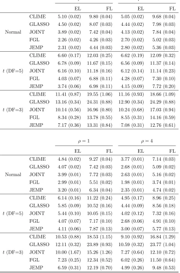
Table 2: Comparison summaries using Entropy loss (EL) and Frobenius loss (FL) over 50
ρ= 0 ρ= 0.25
EL FL EL FL
Normal
CLIME 3.62 (0.02) 6.87 (0.03) 3.92 (0.02) 7.51 (0.04)
GLASSO 2.60 (0.01) 5.03 (0.03) 3.03 (0.01) 5.78 (0.03)
JOINT 2.53 (0.01) 4.97 (0.02) 2.99 (0.01) 5.89 (0.03)
FGL 1.54 (0.01) 2.95 (0.02) 2.21 (0.01) 4.16 (0.02)
JEMP 1.80 (0.01) 3.61 (0.03) 2.48 (0.01) 4.96 (0.03)
t(DF=5)
CLIME 4.77 (0.17) 8.68 (0.26) 5.23 (0.19) 9.63 (0.33)
GLASSO 4.32 (0.09) 8.42 (0.20) 4.82 (0.09) 9.11 (0.18)
JOINT 3.84 (0.12) 7.02 (0.16) 4.43 (0.15) 8.10 (0.21)
FGL 2.54 (0.06) 4.68 (0.10) 3.11 (0.07) 5.62 (0.10)
JEMP 2.60 (0.06) 4.99 (0.11) 3.35 (0.10) 6.44 (0.18)
t(DF=3)
CLIME 9.08 (0.84) 16.05 (1.07) 9.40 (0.92) 15.92 (1.06)
GLASSO 10.64 (0.33) 24.09 (1.06) 11.14 (0.33) 24.26 (1.01)
JOINT 7.54 (0.57) 13.03 (0.87) 8.35 (0.66) 14.09 (0.89)
FGL 5.87 (0.26) 11.39 (0.65) 6.72 (0.30) 12.53 (0.70)
JEMP 5.05 (0.37) 10.10 (0.93) 5.49 (0.30) 10.44 (0.66)
ρ= 1 ρ= 4
EL FL EL FL
Normal
CLIME 4.33 (0.02) 8.33 (0.03) 4.03 (0.02) 7.68 (0.03)
GLASSO 3.52 (0.02) 6.54 (0.03) 3.00 (0.01) 5.67 (0.03)
JOINT 3.50 (0.01) 6.86 (0.02) 2.94 (0.01) 5.78 (0.02)
FGL 2.90 (0.01) 5.37 (0.02) 2.28 (0.01) 4.28 (0.01)
JEMP 3.17 (0.01) 6.40 (0.02) 2.66 (0.01) 5.40 (0.02)
t(DF=5)
CLIME 5.64 (0.16) 10.31 (0.23) 5.20 (0.17) 9.42 (0.26)
GLASSO 5.31 (0.09) 9.81 (0.17) 4.71 (0.09) 8.93 (0.18)
JOINT 4.91 (0.11) 9.09 (0.14) 4.29 (0.12) 7.86 (0.17)
FGL 3.66 (0.06) 6.53 (0.10) 2.98 (0.07) 5.40 (0.10)
JEMP 3.93 (0.07) 7.56 (0.12) 3.27 (0.07) 6.32 (0.14)
t(DF=3)
CLIME 10.00 (0.87) 17.87 (1.16) 9.36 (0.88) 17.25 (1.26)
GLASSO 11.60 (0.32) 23.89 (0.97) 10.89 (0.31) 23.79 (0.99)
JOINT 9.52 (1.68) 14.60 (1.27) 7.57 (0.63) 12.59 (0.71)
FGL 6.71 (0.24) 11.84 (0.52) 6.36 (0.26) 11.87 (0.61)
JEMP 5.90 (0.26) 11.02 (0.59) 5.20 (0.26) 9.70 (0.51)
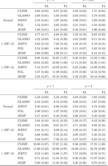
Table 3: Comparison summaries using Entropy loss (EL) and Frobenius loss (FL) over 50
Normal t(DF=5) t(DF=3)
EL FL EL FL EL FL
CLIME 4.39 (0.02) 8.45 (0.04) 6.06 (0.39) 10.82 (0.43) 10.59 (1.03) 17.35 (1.08)
GLASSO 3.62 (0.02) 6.71 (0.03) 5.57 (0.11) 10.02 (0.14) 11.79 (0.43) 24.06 (1.29)
JOINT 3.68 (0.01) 7.16 (0.03) 5.24 (0.14) 9.56 (0.17) 8.28 (0.37) 13.83 (0.50)
FGL 3.12 (0.01) 5.75 (0.02) 3.85 (0.07) 6.84 (0.11) 7.08 (0.33) 12.26 (0.71)
JEMP 3.50 (0.01) 7.04 (0.02) 4.27 (0.08) 8.17 (0.14) 6.22 (0.29) 11.27 (0.60)
Table 4: Comparison summaries using Entropy loss (EL) and Frobenius loss (FL) over 50
replications for Model 4.
To compare performance of five different methods, we use the average entropy loss and the average Frobenius loss defined as,
EL =G−1
G
X
g=1
n
tr(Σ(g)0 Ωˆ(g))−log det(Σ(g) 0 Ωˆ
(g))−po,
FL =G−1
G
X
g=1
kΩ(g)0 −Ωˆ(g) k2 F,
wherek.kF is the Frobenius norm of a matrix.
Table 1 reports the results for Model 1. In terms of estimation accuracy, the three joint estimation methods, JEMP, FGL, and JOINT, outperform the two separate estima-tion methods while JEMP and FGL show better performance than JOINT. In Gaussian cases, FGL exhibits slightly smaller losses than JEMP. However, JEMP outperforms FGL in terms of entropy loss for some cases when the underlying distribution is t5. If the true underlying distribution ist3, then JEMP clearly outperforms FGL in both entropy loss and Frobenius loss for all cases. This indicates that our proposed JEMP can have some ad-vantage in estimation for some non-Gaussian data. Overall, JEMP shows very competitive performance compared with other methods. Tables 2-3 report the results for Models 2 and 3 respectively. Performances of the methods show similar patterns as in Model 1. JEMP and FGL perform best while FGL is slightly better in Gaussian cases and JEMP has the best performance in thet3 case.
0 0.05 0.1 0.15 0.2 0
0.2 0.4 0.6 0.8
Model 1: ρ = 0
CLIME GLASSO JOINT FGL JEMP
0 0.05 0.1 0.15 0.2 0
0.2 0.4 0.6 0.8
Model 1: ρ = 0.25
0 0.05 0.1 0.15 0.2 0
0.2 0.4 0.6 0.8
Model 1: ρ = 1
0 0.05 0.1 0.15 0.2 0
0.2 0.4 0.6 0.8
Model 2: ρ = 0
0 0.05 0.1 0.15 0.2 0
0.2 0.4 0.6 0.8
Model 2: ρ = 0.25
0 0.05 0.1 0.15 0.2 0
0.2 0.4 0.6 0.8
Model 2: ρ = 1
0 0.05 0.1 0.15 0.2 0
0.2 0.4 0.6 0.8
Model 3: ρ = 0
0 0.05 0.1 0.15 0.2 0
0.2 0.4 0.6 0.8
Model 3: ρ = 0.25
0 0.05 0.1 0.15 0.2 0
0.2 0.4 0.6 0.8
Model 3: ρ = 1
0 0.05 0.1 0.15 0.2 0
0.2 0.4 0.6 0.8
Model 1: ρ = 0
0 0.05 0.1 0.15 0.2 0
0.2 0.4 0.6 0.8
Model 1: ρ = 0.25
0 0.05 0.1 0.15 0.2 0
0.2 0.4 0.6 0.8
Model 1: ρ = 1
CLIME GLASSO JOINT FGL JEMP
0 0.05 0.1 0.15 0.2 0
0.2 0.4 0.6 0.8
Model 2: ρ = 0
0 0.05 0.1 0.15 0.2 0
0.2 0.4 0.6 0.8
Model 2: ρ = 0.25
0 0.05 0.1 0.15 0.2 0
0.2 0.4 0.6 0.8
Model 2: ρ = 1
0 0.05 0.1 0.15 0.2 0
0.2 0.4 0.6 0.8
Model 3: ρ = 0
0 0.05 0.1 0.15 0.2 0
0.2 0.4 0.6 0.8
Model 3: ρ = 0.25
0 0.05 0.1 0.15 0.2 0
0.2 0.4 0.6 0.8
Model 3: ρ = 1
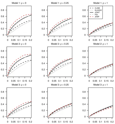
Figures 1-3 show the estimated receiver operating characteristic (ROC) curves averaged over 50 replications. In the Gaussian case of Figure 1, JEMP and FGL show similar per-formance and outperform the others except the case of ρ = 1 in Model 3. In Figures 2 and 3 of multivariatet-distributions, it can be observed that JEMP has better ROC curves when ρ = 0 for all three models. It also shows better performance than the others when
ρ= 0.25 for Models 1-2. Whenρ= 1, all ROC curves move closer together. This is because the true precision matrices become much denser in terms of the number of edges and thus all methods have some difficulty in edge selection. Overall, our proposed JEMP estimator delivers competitive performance in terms of both estimation accuracy and selection.
Note that JEMP and FGL encourage the estimated precision matrices to be similar across all classes. This can be advantageous especially when the true precision matrices have many common values. Therefore, JEMP and FGL can have better performance than JOINT for such problems.
In terms of computational complexity, JEMP can be more intensive than separate es-timation methods and JOINT as it involves a pair of tuning parameters (λ1, λ2) satisfying
λ1 ≤λ2. The computational cost of JEMP can be potentially reduced using the ADMM algorithm discussed in Section 4 with a further improved algorithm for the least squares step.
6. Application on Glioblastoma Cancer Data
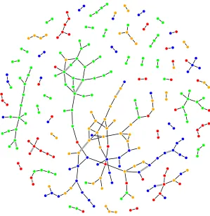
In this section, we apply our joint method to a Glioblastoma cancer data set. The data set consists of 17814 gene expression levels of 482 GBM patients. The patients were classified into four subtypes, namely, classical, mesenchymal, neural, and proneural with sample sizes of 127, 145, 85, and 125 respectively (Verhaak et al., 2010). These subtypes are shown to be different biologically, while at the same time, share similarities as well since they all belong to GBM cancer. In this application, we consider the signature genes reported by Verhaak et al. (2010). They established 210 signature genes for each subtype, which results 840 signature genes in total. These signature genes are highly distinctive for four subtypes and reported to have good predictive power for subtype prediction. In our analysis, the goal is to produce graphical presentation of relationships among these signature genes in each subtype based on the estimation of the precision matrices. Among the 840 signature genes, we excluded the genes with no subtype information or the genes with missing values. As a result, total 680 genes were included in our analysis. To produce interpretable graphical models using our JEMP estimator, we set the values of the tuning parameters asλ1 = 0.30 andλ2= 0.40. JEMP estimated 214 edges shared among all subtypes, 9 edges present only in two subtypes, and 1 edge present only in three subtypes.
The resulting gene networks are shown in Figure 4. The black lines are the edges shared by all subtypes and the thick grey lines are the unique edges present only in two or three subtypes. It is noticeable that most of edges are black lines, which means that they appear in all subtypes. This indicates that the networks of the signature genes reported by Verhaak et al. (2010) may be very similar across all subtypes as they all belong to GBM cancer.
Classical Mesenchymal
Neural Proneural
that are related to many cellular functions. As they are all involved in the same biological process, it may seem reasonable that this network is shared in all GBM subtypes.
The red genes are signature genes for the classical subtype. Likewise, green, blue and orange genes are the mesenchymal, proneural and neural signature genes respectively. Each class of signature genes tends to have more links with the genes in the same class. This is expected because each class of signature genes is more likely to be highly co-expressed.
Each estimated network for each subtype is depicted in Figure 5. The black lines are the edges shared by all subtypes and the colored lines are the edges appearing only in two or three subtypes. One interesting edge is the one between EGFR and MEOX2. It does not appear in the classical subtype while it is shared by all the other subtypes. EGFR is known to be involved in cell proliferation and Verhaak et al. (2010) demonstrated the essential role of this gene in GBM tumor genesis. Furthermore, high rates of EGFR alteration were claimed in the classical subtype. Therefore, studying the relationship between EGFR and MEOX2 can be an interesting direction for future investigation as only the classical subtype lacks this edge.
There are 9 edges appearing only in two subtypes. These include SCG3 and ACSBG1, GRIK5 and BTBD2, NCF4 and CSTA, IFI30 and BATF, HK3 and SLC11A1, ACSBG1 and SCG3, GPM6A and OLIG2, C1orf61 and CKB, and PPFIA2 and GRM1. It would be also interesting to investigate these relationships further as they are unique only in two subtypes. For example, the edge between OLIG2 and GPM6A does not appear in the proneural subtype while it is shared by Neural and Mesenchymal subtypes. High expression of OLIG2 was observed in the proneural subtype (Verhaak et al., 2010), which can down-regulate the tumor suppressor p21. Therefore, it may be helpful to investigate the relationship between OLIG2 and GPM6A for understanding the effect of OLIG2 in the proneural subtype.
Acknowledgments
The authors would like to thank the Action Editor Professor Francis Bach and three review-ers for their constructive comments and suggestions. The authors were supported in part by NIH/NCI grant R01 CA-149569, NIH/NCI P01 CA-142538, and NSF grant DMS-1407241.
Appendix A.
Write Σ(g)0 = (σij,(g)0) and ˆΣ(g)= (ˆσ(g)
ij ). Let mj,0 and r (g)
j,0 be the jth columns ofM0 and R (g) 0 respectively. Define the jth columns of ˆM and ˆR(g) as ˆm
j and ˆr(g)j respectively. We first
state some results established by Cai et al. (2011) in the proof of their Theorem 1.
Lemma 4 Suppose Condition 1 holds. For any fixed g= 1, . . . , G, with probability greater than 1−4p−τ,
max
ij |σˆ (g) ij −σ
(g) ij,0| ≤C0
logp n
1/2 ,
Proof [Proof of Theorem 1] It follows from Lemma 4 that
max
ij |σˆ (g) ij −σ
(g)
ij,0| ≤λ2/(3CM) for all g= 1, . . . , G, (6) with probability greater than 1−4Gp−τ. All following arguments assume (6) holds. First, we have that
|( ˆΩ(g) 1 −Ω
(g)
0 )ej|∞=|Ω (g) 0 (Σ
(g) 0 Ωˆ
(g)
1 −I)ej|∞≤ ||Ω(g)0 ||L 1|(Σ
(g) 0 Ωˆ
(g)
1 −I)ej|∞
≤CM
n
|(Σ(g) 0 −Σˆ
(g)) ˆΩ(g)
1 ej|∞+|( ˆΣ (g)Ωˆ(g)
1 −I)ej|∞
o
≤CM|Ωˆ(g)1 ej|1|Σ(g)0 −Σˆ (g)|
∞+CMλ2
≤ |Ωˆ(g)1 ej|1λ2/3 +CMλ2, for all g = 1, . . . , G. Second, note that {M0, R
(1) 0 , . . . , R
(G)
0 } is a feasible solution of (3) as
|I−Σˆ(g)(M
0+R0(g))|∞ = |(Σ0(g)−Σˆ(g))Ω(g)0 |∞ ≤ ||Ω0(g)||L1|Σ(g)0 −Σˆ(g)|∞ ≤ CMλ2/(3CM) <
λ2 and λ1 =λ2. Therefore, we have that G
X
g=1
|( ˆΩ(g) 1 −Ω
(g)
0 )ej|∞≤ G
X
g=1
|Ωˆ(g)
1 ej|1λ2/3 +GCMλ2≤G
(
|mˆj|1+G−1 G
X
g=1
|ˆr(g) j |1
)
λ2/3 +GCMλ2
≤G (
|mj,0|1+G−1 G
X
g=1
|r(g) j,0|1
)
λ2/3 +GCMλ2
≤G3CMλ2/3 +GCMλ2= 2GCMλ2= 6GCM2 C0(logp/n)1/2.
By the inequality
max ij 1 G G X g=1
|ωˆ(g)ij −ω(g)ij,0|
≤max
j 1 G G X g=1
|( ˆΩ(g)1 −Ω(g)0 )ej|∞≤6CM2 C0
logp n
1/2 ,
the proof is completed.
Lemma 5 With probability greater than 1−2(1 +G)p−τ, the following holds:
max
ij | G
X
g=1
(ˆσij(g)−σij,(g)0)| ≤C0
Glogp
n
1/2 .
Proof We adopt a similar technique used in Cai et al. (2011) for the proof of their Theorem 1. Without loss of generality, we assume thatµ(g)
i = 0 for alli andg. Lety (g) kij :=x
(g) kix
(g) kj −
E(x(g)kix(g)kj). Define ¯x(g)i :=Pn
k=1x (g)
ki/n;i= 1, . . . , p, g= 1, . . . , G. Then
PG
g=1(ˆσ (g) ij −σ
(g) ij,0) =
PG
g=1
Pn
k=1y (g) kij/n−x¯
(g) i x¯
(g) j
any s∈ R, we can show that pr ( 1 n G X g=1 n X k=1 y(g) kij≥η
−1C 1
Glogp
n
1/2)
= pr ( G X g=1 n X k=1 y(g) kij≥η
−1C
1(nGlogp) 1/2
)
≤expn−tη−1C1(nGlogp)1/2
o E ( exp t G X g=1 n X k=1 y(g) kij !)
= exp{−C1logp} G Y g=1 n Y k=1
Enexp(ty(g) kij)
o
= exp
"
−C1logp+ G
X
g=1
nlognEety(g)kij o
#
≤exp
"
−C1logp+ G
X
g=1
nnEety(g)kij
−1o
#
= exp
"
−C1logp+ G
X
g=1
nnEety(g)kij−ty(g)
kij−1
o #
≤exp
(
−C1logp+ G
X
g=1
nt2Ey(g) kij
2
e|ty(g)kij|
)
≤exp
(
−C1logp+ G
X
g=1
(ηG)−1K2logp )
. (7)
The last inequality (7) holds since
nt2E
ykij(g)2e|ty
(g)
kij|
= (ηG)−1(logp)E
η3/2|ykij(g)|2et|y
(g) kij| and E
η3/2|y(g)kij|2et|y
(g)
kij|
≤E
eη3/2|y
(g)
kij|et|y
(g)
kij|
≤E
eη3/2|y
(g)
kij|eη3/2|y
(g)
kij|
≤E
eη|y
(g)
kij|
≤E
eη|x
(g)
kix
(g)
kj|+ηE
|x(g)kix(g)kj|
≤
E
eη|x
(g) kix (g) kj| 2 ≤ E eηx (g) ki 2
/2+ηx(g)kj2/22
≤E
eηx(g)ki
2 E eηx (g) kj 2
≤K2.
From (7), it follows that
pr 1 n G X g=1 n X k=1
y(g)kij ≥η−1C1
Glogp
n
1/2
Therefore, we have pr max ij 1 n G X g=1 n X k=1 y(g) kij
≥η−1C1
Glogp
n
1/2
≤2p−τ. (8)
Next, letC2= 2 +τ+η−1(eK)2. Cai et al. (2011) showed in the proof of their Theorem 1 that
pr
max
ij |x¯ (g) i x¯
(g) j | ≥η
−2C2
2logp/n
≤2p−τ−1.
Using this result, we have that
pr max ij | G X g=1 ¯
x(g)i x¯(g)j | ≥η−2C22Glogp/n
≤pr G X g=1 max
ij |x¯ (g) i x¯
(g) j | ≥η
−2C2
2Glogp/n
≤ G X g=1 pr max
ij |x¯ (g) i x¯
(g) j | ≥η
−2C2
2logp/n
≤
G
X
g=1
2p−τ−1≤2Gp−τ (9)
By (8), (9) and the inequalityC0> η−1C1+η−2C22(Glogp/n)1/2, we see that
pr max ij | G X g=1 (ˆσ(g)
ij −σ (g)
ij,0)| ≥C0
Glogp
n
1/2 ≤pr max ij 1 n G X g=1 n X k=1 y(g) kij
≥η−1C1
Glogp
n
1/2 + pr max ij | G X g=1 ¯
x(g)i x¯(g)j | ≥η−2C22Glogp/n
≤2(1 +G)p−τ.
The proof is completed.
Proof [Proof of Theorem 2] By Lemma 4 and 5, we see that
max
ij | G
X
g=1 (ˆσ(g)
ij −σ (g)
ij,0)| ≤C0
Glogp
n
1/2
and max
ij |σˆ (g) ij −σ
(g) ij,0| ≤C0
logp n
1/2
, (10)
for allg= 1, . . . , Gwith probability greater than 1−2(1 + 3G)p−τ. All following arguments assume (10) holds. Note that{M0, R(1)0 , . . . , R
(G)
0 }is a feasible solution of (3) as
|I −Σˆ(g)
(M0+R0(g))|∞=|(Σ (g) 0 −Σˆ
(g)
)Ω(g)0 |∞≤ ||Ω(g)0 ||L
1|Σ (g) 0 −Σˆ
(g)| ∞
and
|G−1
G
X
g=1
n
I−Σˆ(g)(M
0+R0(g))
o |∞
≤ |G−1
G
X
g=1 (Σ(g)
0 −Σˆ (g))M
0|∞+|G−1
G
X
g=1 (Σ(g)
0 −Σˆ (g))R(g)
0 |∞
≤ ||M0||L1|G
−1 G
X
g=1 (Σ(g)
0 −Σˆ (g))|
∞+G−1
G
X
g=1
||R(g) 0 ||L1|Σ
(g) 0 −Σˆ
(g)|
∞
≤CMC0{logp/(nG)}1/2+CRC0{logp/(nG)}1/2=λ1.
Now, we find an upper bound of|G( ˆM−M0)ej|∞=|PGg=1( ˆΩ(g)1 −Ω(g)0 )ej|∞. In particular,
we use
|
G
X
g=1 ( ˆΩ(g)
1 −Ω (g)
0 )ej|∞≤ |
G X g=1 Ω(g) 0 (Σ (g) 0 −Σˆ
(g)) ˆΩ(g)
1 ej|∞+|
G
X
g=1 Ω(g)
0 ( ˆΣ (g)Ωˆ(g)
1 −I)ej|∞. (11)
First, consider the first term in the right-hand side of (11). We can show that
| G X g=1 Ω(g) 0 (Σ (g) 0 −Σˆ
(g)) ˆΩ(g)
1 ej|∞≤ |
G
X
g=1
M0(Σ(g)0 −Σˆ (g)) ˆm
j|∞+|
G X g=1 M(g) 0 (Σ (g) 0 −Σˆ
(g))ˆr(g) j |∞
+| G X g=1 R(g) 0 (Σ (g) 0 −Σˆ
(g)) ˆm j|∞+|
G X g=1 R(g) 0 (Σ (g) 0 −Σˆ
(g))ˆr(g) j |∞
≤ ||M0||L1
( | G X g=1 (Σ(g)
0 −Σˆ (g))|
∞|mˆj|1+ G
X
g=1
|Σ(g) 0 −Σˆ
(g)|
∞|rˆ(g)j |1
)
+ G
X
g=1
|R(g) 0 (Σ
(g) 0 −Σˆ
(g))|
∞|mˆj|1+ G
X
g=1
|R(g) 0 (Σ
(g) 0 −Σˆ
(g))|
∞|rˆ(g)j |1.
Using the assumptions ||R(g)0 ||L1 ≤CR and
PG
g=1||R (g)
0 ||L1 ≤G 1/2C
R, we have
| G X g=1 Ω(g) 0 (Σ (g) 0 −Σˆ
(g)) ˆΩ(g)
1 ej|∞≤CMC0(Glogp/n)1/2|mˆj|1+CMC0(logp/n)1/2 G
X
g=1
|rˆ(g) j |1
+CRC0(Glogp/n)1/2|mˆj|1+CRC0(logp/n)1/2 G
X
g=1
|rˆ(g) j |1
≤C0(CM +CR)(Glogp/n)1/2(|mˆj|1+G−1/2 G
X
g=1
|ˆr(g) j |1)
≤C0(CM +CR)(Glogp/n)1/2(|mj,0|1+G−1/2 G
X
g=1
|r(g) j,0|1)
For the second term in the right-hand side of (11), note that
|
G
X
g=1 Ω(g)
0 ( ˆΣ (g)Ωˆ(g)
1 −I)ej|∞
≤ |
G
X
g=1
M0( ˆΣ(g)Ωˆ(g)−I)ej|∞+|
G
X
g=1
R(g)0 ( ˆΣ(g)ˆ Ω(g)−
I)ej|∞
≤ ||M0||L1| G
X
g=1 ( ˆΣ(g)ˆ
Ω(g)−
I)ej|∞+
G
X
g=1
||R(g)0 ||L
1|( ˆΣ (g)ˆ
Ω(g)−
I)ej|∞
≤CMλ1+G1/2CRλ2 =C0CM(CM + 2CR)(Glogp/n)1/2. (13)
By (11), (12), (13) and the equality |Mˆ −M0|∞= maxj|( ˆM−M0)ej|∞ , we have
|Mˆ −M0|∞≤C0(2CM2 + 4CMCR+CR2)
logp nG
1/2 .
The proof is completed.
Proof [Proof of Theorem 3] By Theorem 1, we see that
max
ij G
X
g=1
|ωˆij(g)−ω(g)ij,0| ≤2GCMλ2≤δn, (14)
with probability greater than 1−4Gp−τ. We show that S0 = ˆS when (14) holds. For any (i, j, g) ∈/ S0, we have |ωˆij(g)|= |ωˆ(g)ij −ω(g)ij,0| ≤ PGg=1|ωˆij(g)−ωij,(g)0| ≤ δn. Therefore, we
see ˜ωij(g) = 0, which implies ˆS ⊂ S0. On the other hand, for any (i, j, g) ∈ S0, we have
|ωˆ(g)ij | ≥ |ω(g)ij,0| − |ωˆij(g) −ωij,(g)0| ≥ |ωij,(g)0| −PG
g=1|ωˆ (g) ij −ω
(g)
ij,0| > δn. Therefore, we see that
˜
ωij(g)6= 0, which impliesS0 ⊂Sˆ. In summary, we see thatS0= ˆSif (14) holds, which implies that pr(S0 = ˆS)≥pr(maxijPGg=1|ωˆ
(g) ij −ω
(g)
ij,0| ≤δn).
References
Onureena Banerjee, Laurent El Ghaoui, and Alexandre d’Aspremont. Model selection through sparse maximum likelihood estimation for multivariate gaussian or binary data. Journal of Machine Learning Research, 9:485–516, 2008.
Stephen Boyd and Lieven Vandenberghe. Convex Optimization. Cambridge University Press, Cambridge, 2004.
Tony Cai, Weidong Liu, and Xi Luo. A constrained l1 minimization approach to sparse precision matrix estimation. Journal of the American Statistical Association, 106:594– 607, 2011.
Patrick Danaher, Pei Wang, and Daniela M. Witten. The joint graphical lasso for inverse covariance estimation across multiple classes. Journal of the Royal Statistical Society, Series B, 76:373–379, 2014.
Theodoros Evgeniou and Massimiliano Pontil. Regularized multitask learning. In Proceed-ings of the tenth ACM SIGKDD international conference on Knowledge discovery and data mining, pages 109–117, Seattle, Washington, 2004.
Jianqing Fan and Runze Li. Variable selection via nonconcave penalized likelihood and its oracle properties. Journal of the American Statistical Association, 96:1348–1360, 2001.
Jianqing Fan, Yang Feng, and Yichao Wu. Network exploration via the adaptive lasso and scad penalties. The Annals of Applied Statistics, 3:521–541, 2009.
Jerome Friedman, Trevor Hastie, and Robert Tibshirani. Sparse inverse covariance estima-tion with the graphical lasso. Biostatistics, 9:432–441, 2008.
Jian Guo, Elizaveta Levina, George Michailidis, and Ji Zhu. Joint estimation of multiple graphical models. Biometrika, 98:1–15, 2011.
Jean Honorio and Dimitris Samaras. Simultaneous and group-sparse multi-task learning of gaussian graphical models. arXiv:1207.4255, 2012.
Clifford Lam and Jianqing Fan. Sparsistency and rates of convergence in large covariance matrix estimation. The Annals of Statistics, 37:4254–4278, 2009.
Wonyul Lee, Ying Du, Wei Sun, David Neil Hayes, and Yufeng Liu. Multiple response regression for gaussian mixture models with known labels. Statistical Analysis and Data Mining, 5:493–508, 2012.
Nicolai Meinshausen and Peter B¨uhlmann. High-dimensional graphs and variable selection with the lasso. The Annals of Statistics, 34:1436–1462, 2006.
Haotian Pang, Han Liu, and Robert Vanderbei. fastclime: A fast solver for parameterized lp problems and constrainedl1-minimization approach to sparse precision matrix estimation, 2014. R package version 1.2.4.
Jie Peng, Pei Wang, Nengfeng Zhou, and Ji Zhu. Partial correlation estimation by joint sparse regression models. Journal of the American Statistical Association, 104:735–746, 2009.
Pradeep Ravikumar, Martin J. Wainwright, Garvesh Raskutti, and Bin Yu. High-dimensional covariance estimation by minimizingl1-penalized log-determinant divergence. Electronic Journal of Statistics, 5:935–980, 2011.
The Cancer Genome Atlas Research Network. Comprehensive genomic characterization defines human glioblastoma genes and core pathways. Nature, 455:1061–1068, 2008.
Roel G.W. Verhaak, Katherine A. Hoadley, Elizabeth Purdom, Victoria Wang, Yuan Qi, Matthew D. Wilkerson, C. Ryan Miller, Li Ding, Todd Golub, Jill P. Mesirov, Gabriele Alexe, Michael Lawrence, Michael OKelly, Pablo Tamayo, Barbara A. Weir, Stacey Gabriel, Wendy Winckler, Supriya Gupta, Lakshmi Jakkula, Heidi S. Feiler, J. Graeme Hodgson, C. David James, Jann N. Sarkaria, Cameron Brennan, Ari Kahn, Paul T. Spellman, Richard K. Wilson, Terence P. Speed, Joe W. Gray, Matthew Meyerson, Gad Getz, Charles M. Perou, D. Neil Hayes, and The Cancer Genome Atlas Research Net-work. Integrated genomic analysis identifies clinically relevant subtypes of glioblastoma characterized by abnormalities in PDGFRA, IDH1, EGFR, and NF1. Cancer Cell, 17: 98–110, 2010.
Ming Yuan. High dimensional inverse covariance matrix estimation via linear programming. Journal of Machine Learning Research, 11:2261–2286, 2010.