Integrating a Partial Model into Model Free Reinforcement Learning
Aviv Tamar [email protected]
Dotan Di Castro [email protected]
Ron Meir [email protected]
Department of Electrical Engineering Technion
Haifa 32000, Israel
Editor:Peter Dayan
Abstract
In reinforcement learning an agent uses online feedback from the environment in order to adaptively select an effective policy. Model free approaches address this task by directly mapping environmen-tal states to actions, while model based methods attempt to construct a model of the environment, followed by a selection of optimal actions based on that model. Given the complementary advan-tages of both approaches, we suggest a novel procedure which augments a model free algorithm with a partial model. The resultinghybridalgorithm switches between a model based and a model free mode, depending on the current state and the agent’s knowledge. Our method relies on a novel definition for a partially known model, and an estimator that incorporates such knowledge in or-der to reduce uncertainty in stochastic approximation iterations. We prove that such an approach leads to improved policy evaluation whenever environmental knowledge is available, without com-promising performance when such knowledge is absent. Numerical simulations demonstrate the effectiveness of the approach on policy gradient and Q-learning algorithms, and its usefulness in solving a call admission control problem.
Keywords: reinforcement learning, temporal difference, stochastic approximation, markov deci-sion processes, hybrid model based model free algorithms
1. Introduction
In Reinforcement Learning (RL) an agent attempts to improve its performance over time at a given task, based on continual interaction with the (usually unknown) environment, (Bertsekas and Tsit-siklis, 1996; Sutton and Barto, 1998). This improvement takes place by modifying the action se-lection policy, based on feedback from the environment and prior knowledge available to the agent. Formally, RL is often phrased as the problem of finding a mapping, the so calledpolicy, from the environment’s states to the agent’s actions that maximizes a given functional of a reward function.
states to actions. In this sense, no model of the environmental dynamics is required. While it can be shown that both approaches, under mild conditions, asymptotically reach the same optimal policy on typical MDP’s, it is known that each approach possesses distinct merits. Model based meth-ods often make better use of a limited amount of experience and thus achieve a better policy with fewer environmental interactions. On the other hand, model free methods are simpler, require less computational resources, and are not affected by biases in the design (or estimation) of the model.
The view taken in this work is that this dichotomy between algorithmic approaches, although popular, is not necessarily desirable. As an example, consider a scenario where some parts of the environment are known in advance, but computational resources are limited, restricting the use of proper model based approaches. In this case, ahybrid approachmay allow us to benefit from using parts of the model in the algorithm, without sacrificing its simplicity, thus striking a balance between the merits of each approach. Surprisingly, the concept of combining model free and model based algorithms has received very little attention in the RL literature, and theoretical guarantees to its advantages are lacking.
In this work we pursue such a hybrid approach applicable to cases where partial model infor-mation is available in a specific form which we termpartially known MDP. We provide a method for integrating such information into RL algorithms of the Stochastic Approximation (SA) type (Kushner and Yin, 2003; Borkar, 2008). This class of online model free algorithms includes many standard RL approaches that have been used effectively in practice (e.g., Tesauro, 1995; Crites and Barto, 1996). The method we propose reduces uncertainty in the algorithm trajectory, thereby improving its performance. Our theoretical analysis focuses on a particular model free algorithm -the well known TD(0) policy evaluation algorithm, and we prove that our hybrid method leads to improved performance, as long as sufficiently accurate partial knowledge is available. The effec-tiveness and generality of our method is further demonstrated in two numerical simulations. In the first, we apply it to a policy gradient type algorithm, and investigate its performance in randomly generated MDPs. In the second, we consider a call admission control problem. As it turns out, our partially known MDP definition is a natural choice for describing plausible partial knowledge in such problems, and performance improvement is demonstrated for a Q-learning algorithm.
1.1 A High-Level Sketch of the Method
1.2 Related Work
One difficulty of RL is coping with the stochasticity inherent to RL algorithms. In this work we de-fine a partially known MDP, and use this partial knowledge to improve the asymptotic performance of stochastic approximation type algorithms. Our method is novel, and specifically deals with this difficulty. We note that a different notion of a partially known MDP was used by Kearns and Singh (2002) and Brafman and Tennenholtz (2003) to tackle a different difficulty of RL - the ‘exploration exploitation’ tradeoff. Thus, the partial model which we use only to reduce stochastic fluctuations may further be used to explore or exploit more efficiently. On the other hand, the advantage of our approach is that it is general, and may be easily applied to a large class of model free algorithms.
When a full model of state transitions is available, applying our method to Q-learning results in an algorithm known as Real Time Dynamic Programming (RTDP) (Barto et al., 1995). Thus, the method presented in this work may be viewed as a bridge between the model free Q-Learning and the model based RTDP.
In Section 4 we analyze the asymptotic fluctuations in a fixed step TD(0) algorithm with a partial model. A similar analysis of TD(0) without partial model was given by Dayan and Sejnowski (1994) for a decreasing step size and without explicit convergence rate results, and by Konda (2002) using a similar technique to bound the convergence rate. Singh and Dayan (1998) provided update equations for the MSE of TD(0), which we use as a measure of convergence rate, though their equations were only solvable by simulation. This work presents explicitvaluesof the asymptotic MSE.
On a slightly different note, an early approach towards a hybrid model based - model free RL algorithm is the Dyna architecture (Sutton, 1990), in which interactions with the environment are used both for a direct policy update, using a model free RL algorithm, and for an update of an environmental model. This model is then used to generate simulated trajectories which are fed to the same model free algorithm for further policy improvement. In a more recent work by Abbeel et al. (2006), a hybrid approach is proposed that combines policy search on an inaccurate model, with policy evaluations in the real environment. Finally, we note that the idea of combining model based and model free approaches has been proposed in the context of animal and human learning, suggesting an explanation for behavioral choice experiments (Daw et al., 2005). To the best of our knowledge, our work presents the first formal proof of theadvantageof a hybrid algorithm over a standard model free algorithm.
1.3 Organization
2. Estimation of a Random Variable Mean with Partial Knowledge
Our method of using partial knowledge in an SA algorithm is based on constructing a better esti-mator for the mean update at each step. In this section we describe our estiesti-mator in the context of estimating the mean of a random variable. This allows us to derive all its important properties without the notational burden of the SA setting. The results we derive will then easily transfer to the more complicated SA setting.
LetXbe a random variable over a finite and discrete setΩand letP(ω),Pr(X=ω)denote the probability distribution ofX. SinceP(ω)contains all the information aboutX, a natural definition for partial knowledge in this setting is information regarding some of its attributes. In particular, we assume that for an a-priori given subset ofΩ, the ratios between the probability distribution values are provided. Denote byKthis set for which the ratios ofPare known,1
K,
ω:ω∈Ω s.t. P(ω)
∑ ω′∈KP(
ω′) is known
. (1)
We refer toK as thepartial knowledgeset. Suppose we are given one sample ofX, denoted byx, and we wish to estimate (without bias) the expectationµ=E[X],∑ω∈ΩωP(ω). Our estimator can
be any function ofx, and of values and probability ratios in the partial knowledge setK.
The Maximum Likelihood (ML) estimator ofµis derived by first usingxto generate the ML esti-mate of the complete probability distribution ˆP(ω), and then calculating the expectation∑ωωPˆ(ω). For a given known setK, let
P
K(ω)denote the set of all probability distributionsP(ω)that satisfythe ratios in (1). If the observed sample x is not inK, then the ML estimate for the probability distribution ˆP(ω;x∈/K)is given by
ˆ
P(ω;x∈/K) = argmax P(ω)∈PK(ω)
P(x) =δx,ω, (2)
whereδx,ωis Kronecker’s delta. Conversely, ifxis inK, the ML estimate ˆP(ω;x∈K)is
ˆ
P(ω;x∈K) = argmax P(ω)∈PK(ω)
P(x) = 1
K
ωP(ω) ∑ ω′∈KP(ω
′), (3)
where 1K
ω denotes the indicator function that equals 1 if ω∈K and 0 otherwise. Letting ¯K
denote the complement of the setK, combining (2) and (3) gives the ML estimate for the probability distribution ˆP(ω)
ˆ
P(ω;x) =1K
x
1K
ωP(ω) ∑ ω′∈KP(ω
′)+1 ¯
K
xδx,ω. (4)
By taking an expectation of (4), we derive the ML estimate forµgiven the partial knowledge, which we denote by ˆµK
ˆ
µK(x) =1 K
x·
E[X·1K X]
E[1K X]
+1K¯
x·x. (5)
Note that (5) uses the partial knowledge in a very intuitive way. It ‘replaces’ samples in the known set with their weighted average, which by (1) is known. An important property of the esti-mator ˆµK is that it is unbiased, as expressed in the following Lemma.
Lemma 1 The estimatorµˆKis unbiased, namelyE[ˆµK] =µ.
Proof By direct calculation
E[ˆµK] = E[1 K X]·
E[X·1K X]
E[1K
X]
+E1K¯ X·X
= EX 1K X+1
¯
K X
=E[X].
In the following Lemma the Mean Squared Error (MSE) of ˆµKis computed. LetP(K) =∑ω∈KP(ω),
and letPK(ω)denote the probability measure over the known setK, namely
PK(ω),1 K
ωP(ω)/P(K).
Denote by EK[·]and VarK[·]the expectation and variance under the probability measurePK.
Lemma 2 The MSE ofµˆKisE
h
(µˆK−µ)
2i=Var[X]
−P(K)·VarK[X].
Proof Observe that for any function f(·) EK
h
(f(X)−µ)2i = EK
h
(f(X)−EKf(X) +EKf(X)−µ)
2i
= VarKf(X) + (EK[f(X)]−µ)
2
, (6)
where the cross terms in the second equality vanish. Next, we have
E[ˆµK(X)−µ]
2 = Eh 1K X+1
¯
K X
(µˆK(X)−µ)
2i
= P(K)EK
h
(µˆK(X)−µ)
2i
+E
h
1K¯
X(X−µ)
2i
= P(K) (EK[X]−µ)
2+Eh1K¯
X(X−µ)
2i
= P(K)EK
h
(X−µ)2i−VarK[X]
+E
h
1K¯
X(X−µ)
2i
= E
h
(X−µ)2i−P(K)·VarK[X],
where in the fourth equality we used (6) with f(X) =X.
One could disregard the partial knowledge altogether, and choose to use the samplex itself as an unbiased estimate forµ. Denote this estimator, which will be referred to as the sample estimator, by
ˆ
µ(x) =x. (7)
Var[X], and from Lemma 2 we deduce that when the cardinality of the known set satisfies|K|>1, andP(K)>0, the MSE of ˆµK is smaller than that of ˆµ. In parameter estimation parlance, we say
that ˆµKdominatesµˆ (Schervish, 1995).
As will be shown in the next section, the update at each iteration of an SA algorithm can be seen as the estimation of an expected update direction. This estimation is based on one sample, obtained through observation of the system dynamics at that step, and the estimator used is just ˆµ. When partial knowledge of these dynamics is available, we propose to use ˆµKinstead, and benefit from its
reduced variance.
An appropriate question at this point is whether a better estimator than ˆµK exists. We refer the
interested reader to appendix A, where we show that ˆµKis admissible. For the following discussion
however, the results of Lemmas 1 and 2 suffice.
3. A Stochastic Approximation Algorithm with Partial Model Knowledge
In this section we describe our method of endowing a model free RL algorithm with partial model knowledge. We start with some general definitions of the RL environment and SA algorithms. Then, we consider a situation where partial knowledge of the environment model is available. Based on the estimator developed in the previous section, we propose a general form of SA algorithms that incorporate such knowledge.
3.1 Preliminaries
We describe the notation used throughout the paper, the RL environment, and the stochastic approx-imation method.
3.1.1 NOTATION
Throughout the rest of the paper the following notation is used. All vectors are column vectors, and (·)T denotes the transpose operator. The productA◦Bdenotes the element-wise product (Hadamard product) ofAandB. Tr[·]is the trace of a matrix. The cardinality of a setKis denoted by|K|, and its complement by ¯K.Unless noted otherwise, a subscript of a variable denotes time. Thei-th element of a vectorAis denoted by[A]i orA(i), depending on the context. The(i,j)element of a matrixB
is denoted by[B]i j.
3.1.2 RL ENVIRONMENT
We consider an agent interacting with an unknown environment, modeled by an MDP in discrete time with a finite state set
X
and action setU
. Each selected actionu∈U
at a statex∈X
determinesa stochastic transition to the next statey∈
X
with a probabilityPu(y|x).For each statexthe agent receives a corresponding deterministic rewardr(x), which is bounded by rmax, and depends only on the current state.2 The agent maintains apolicy function, µθ(u|x),
parametrized by a vectorθ∈RL, mapping a statexinto a probability distribution over the actions
U
. Under policyµθ, the environment and the agent induce a Markovian transition matrix, denoted byPµθ, which we assume to be ergodic.
3 This Markovian transition matrix has a stationary distribution 2. Generalizing the results presented here to state-action rewards is straightforward. Generalization to stochastic rewards
over the state space
X
, denoted byπµθ. LetΠµθ∈R| X|×|X|
be a diagonal matrix where its elements are Πµθ =diag(πµθ). Our goal is to optimize θwith respect to some performance criteria. The tuning ofθis performed online in the following fashion. At time n, the current parameter value equalsθnand the agent is in statexn. It then chooses an actionunaccording toµθn(u|xn), observes
xn+1, and updatesθn+1according to some protocol.
3.1.3 STOCHASTICAPPROXIMATION
Stochastic approximation methods (Kushner and Yin, 2003; Borkar, 2008) are a class of iterative stochastic algorithms, to which many model free RL algorithms belong (Bertsekas and Tsitsiklis, 1996). Analysis of SA methods has received considerable attention over the past few decades, and many analysis techniques are available. In particular, the ODE approach introduced by Ljung (1977), is a widely used method for investigating the asymptotic behavior of SA iterates. The algorithms that we deal with in this paper are all cast in the following SA form,4
θn+1=θn+εnF(θn,xn,un,xn+1), (8)
where{εn}are positive step sizes. The key idea of the technique is the following. Iterate (8) can be decomposed into a deterministic function of the current state, action and parameter, denoted by
g(θn,xn,un), and a martingale difference noise termδMn,
θn+1=θn+εn(g(θn,xn,un) +δMn), (9)
whereg(θn,xn,un),E[F(θ,xn,un,xn+1)|θn,xn,un],δMn,F(θn,xn,un,xn+1)−g(θn,xn,un), and the expectation is taken over the next statexn+1.
Suppose that the effect of the martingale difference noise weakens due to repeated averaging,
and further assume that there exists a continuous function ¯g(θ) such that m1m+∑n−1
i=n
g(θ,xi,ui) →
¯
g(θ)w.p.1 asm,n→∞.5 Consider the following ordinary differential equation (ODE)
dθ/dt=g¯(θ). (10)
Then, a typical result of the ODE method in the SA setup suggests that the asymptotic limits of (8) and (10) are identical. Another aspect of SA relates to the rate of convergence of such iterates (Kushner and Yin, 2003), an issue that will be elaborated on later.
3.1.4 A NOTE ONTYPES OFCONVERGENCE
The type of convergence to the asymptotic limit depends primarily on the step size used. Let θ∗
denote an asymptotically stable fixed point of (10), and assume that it is unique. Then, for a suitably decreasing step size, convergence w.p. 1 ofθntoθ∗can be established. For a constant step size,θn can be shown to converge weakly to a random variable centered onθ∗. In the following we use the term convergence ambiguously, and the precise definition should be inferred from the context. For a detailed and rigorous discussion of the types of convergence in SA the reader is referred to Kushner and Yin (2003).
4. This is not the most general SA form, but one that is cast to the RL setup.
5. Note that for stationary policies, the strong law of large numbers for Markov chains may be used to write ¯gexplicitly ¯
3.2 Partial Model Based Algorithm
A key observation obtained from examining Equations (8-9), is that F(θn,xn,un,xn+1) in the SA
algorithm is just the sample estimator (7) ofg(θn,xn,un), the mean update at each step. The esti-mation variance in this case stems from the stochastic transition fromxn toxn+1. In the following
we assume that we have, prior to running the algorithm, some information about these transitions in the form of partial transition probability ratios. Similarly to Section 2, define the known set for statexand actionuas
Kx,u,
y:y∈
X
s.t. Pu(y|x) ∑y′∈Kx,uPu(y
′|x) is known
. (11)
We refer to the known sets for all states and actions as thepartially known MDP.
It is clear that definition (11) is motivated by the theoretical results presented in Section 2, and at this point it may well be questioned whether such a definition has any use in practice. We refer the concerned reader to Section 6, where it is shown that in certain problems definition (11) arises as thenaturalrepresentation of partial model knowledge.
Denote by1K
n+1 an indicator function that equals 1 if{xn+1}belongs toKxn,un and 0 otherwise.
Based on the estimator introduced in Section 2, we propose the following update rule for the tunable parameter, denoted byθK, which we refer to as theIntegrated Partial Model(IPM) iteration
θK
n+1=θ
K
n+εn 1Kn+1F
K
n +1¯
K
n+1F(θ
K
n,xn,un,xn+1)
, (12)
where, abusing notation,FK
n =FnK(θKn,xn,un), and
FK
n ,
∑
y∈Kxn,un
Pun(y|xn)F(θ K
n,xn,un,y)
∑
y∈Kxn,un
Pun(y|xn)
. (13)
Similarly to (9), iterate (12) can also be decomposed into a mean functiongK(θK
n,xn,un)and a martingale difference noiseδMK
n
θK
n+1=θKn+εn(gK(θKn,xn,un) +δMKn),
and by Lemma 1 we havegK(θ,x,u) =g(θ,x,u). Similarly, defining ¯gK(θ) =E[gK(θ,x,u)
|θ]we
get that ¯gK(θ) =g¯(θ), and we reach the following important conclusion, which is summarized as a
theorem.
Theorem 3 The IPM iteration defined in(12)leads to the same characteristic ODE dθ/dt=g¯(θ)
as the regular SA iteration(8).
3.3 Step Size Considerations
As it turns out, the improvement in performance attained by the IPM iteration is heavily influenced by the step size used. This can be intuitively explained using the following example. Let{zi}be a sequence of i.i.d. bounded random variables, with meanµzand varianceσ2z. Consider the following SA iteration
θn+1=θn+εn(zn+1−θn).
For a decreasing step size of the formεn=1/(n+1), the value ofθnis simply the empirical average, which converges w.p. 1 to µz. As a performance measure, consider the MSE defined by Ekθn−µzk2, which equals σ2z/n. Integration of partial knowledge based on (12) in this case is equivalent to averaging variables with the same mean but with a reduced variance, and the MSE still approaches zero at a rateO(1/n). On the other hand, when the step size is constant,θnconverges in mean toµz, but the MSE converges to a non-zero value which, intuitively, is proportional6to the varianceσ2
z. Any variance reduction in this case would thus prove valuable.
The use of a constant step size, though clearly undesirable in the preceding example, is quite common in RL applications, as it allows the iterates to quickly reach a neighborhood of the desired solution, and can cope with time varying environments. In the following discussion, we shall thus focus our analysis on algorithms with a constant step size.
4. TD(0) with Partial Model Knowledge
In this section we apply our IPM method of Equation (12) to the well known model free algorithm Temporal Difference (TD(0); Sutton and Barto, 1998). The simplicity of TD(0) allows us to math-ematically characterize its performance in terms ofconvergence rate, and to quantify the impact of using the IPM method on it. The mathematical results we derive specifically for TD(0) are also characteristic of more complex algorithms, as will be shown in subsequent sections.
4.1 Definitions
Throughout this section, we assume that the agent’s policyµis deterministic and fixed, mapping a specific action to each state, denoted byu(x).
4.1.1 VALUEFUNCTIONESTIMATION
Letting 0<γ<1 denote a discount factor, define the value function for statexunder policyµas the expected discounted return when starting from statexand executing policyµ
Vµ(x),E
"
∞
∑
t=0γtr(xt)
x0=x
#
.
Since in this section the policyµis constant, from now on we omit the superscriptµinVµ(x), and the subscriptµinPµ,πµ, andΠµ.
The value function is a vector of size|
X
|. When the state space is large, Function Approximation(FA) is often used to find an approximation to the value function in a subspace of sizeL<|X|. Linear
FA is implemented as follows. Given a set of|X|linearly independent basis vectorsφ(x)∈RL, the goal is to find an approximation toV(x), denoted by ˆV(x,θ)and defined as
ˆ
V(x,θ) =φ(x)Tθ.
Note that the tunable parameter θin this case is a vector of Llinear weights. In vector form we write ˆV(θ) =Φθ, whereΦ∈R|X|×Lis a matrix composed of rows of basis vectors.
Define theTemporal Difference(TD) at timenas
dn,r(xn) +γφ(xn+1)Tθn−φ(xn)Tθn.
For some small step sizeε, the fixed step TD(0) algorithm updatesθonline in the following manner,
θn+1 = θn+εdnφ(xn). (14)
This is an SA algorithm as defined in (8), and its associated ODE is (Bertsekas and Tsitsiklis, 1996, Lemma 6.5)
dθ
dt =b+Aθ. (15)
where
A , ΦTΠ(γP−I)Φ, (16)
b , ΦTΠr.
Equation (15) is linear and has a fixed pointθ∗that satisfies Aθ∗=−b.
Furthermore, the eigenvalues of A all have a negative real part (Bertsekas and Tsitsiklis, 1996, Lemma 6.6b), and thereforeθ∗is a unique and stable fixed point.
4.1.2 INTEGRATEDPARTIALMODELTD(0)
We now use the method developed in Section 3 to integrate a partial model into the TD(0) algorithm. Since the policy is deterministic we drop theusubscript in the known set definition. Using (12) and (13) we define IPM-TD(0)
θK
n+1 = θ
K
n+εd
K
nφ(xn),
dK
n , r(xn) +γ 1Kn+1F
K
n +1
¯
K
n+1φ(xn+1)TθKn
−φ(xn)TθKn, (17)
FK
n ,
∑
y∈Kxn
P(y|xn)φ(y)TθK
n
∑
y∈Kxn
P(y|xn) .
Using Theorem 3 we conclude that the IPM-TD(0) iterates have the same characteristic ODE as the TD(0) iterates of Equation (14), and therefore converge to the same fixed pointθ∗of (15).
4.2 Performance Improvement Proof
In this section we prove that the performance of the IPM-TD(0) iteration is superior in terms of asymptotic MSE to regular TD(0). The formal approach we follow here may be carried out for other SA algorithms as well, though the expressions involved may become more complicated.
Recall that the asymptotic limit point of both regular TD(0) and IPM-TD(0) isθ∗. A natural
performance measure in this case is the asymptotic MSE defined by
lim
n→∞Ekθn−θ ∗k2.
The remainder of this section is devoted to showing that integrating a partial model reduces the asymptotic MSE, namely
lim n→∞Ekθ
K
n−θ∗k
2
<lim
n→∞Ekθn−θ ∗k2
,
whenever the known setKis not null.
By Lemma 2, at each iteration step we are guaranteed (as long as our partial model is not null) a reduction in the noise variance. This clearly indicates that some improvement in the asymptotic MSE can be expected, but a precise quantification of this is more complicated. A powerful tool for this task is the rate of convergence theory for SA (or a ‘limit theorem for fluctuations’, as termed by Borkar, 2008). In their treatment of rate of convergence, Kushner and Yin (2003, p. 315) discuss the properties of the sequence
ρn,(θn−θ∗)/√ε. (18)
Application of their Theorem 10.1.3 to the TD(0) iteration results in the following theorem.
Theorem 4 The sequenceρn converges in distribution, asε→0and n→∞such that nε→∞,7
to a normally distributed random variable, which is the stationary distribution of the stochastic differential equation
dU=AU dt+dW. (19)
A is defined in(16), and W is a Wiener process with covariance matrixΣ=Σ0+Σ1+ΣT
1 where Σ0= lim
n→∞E
h
(dnφ(xn)) (dnφ(xn))T
θn=θ
∗i, (20)
Σ1= ∞
∑
j=1lim n→∞E
h
(dnφ(xn)) (dn+jφ(xn+j))T
θn=θn+j=θ
∗i.
For the IPM iteration(17)we haveΣK
0,ΣK1where dnKreplaces dnin(20).
The proof of Theorem 4 consists of verifying a lengthy set of technical assumptions required for Theorem 10.1.3 of Kushner and Yin (2003), and is fully described in Appendix E.
The stationary solution to (19) is normally distributed with zero mean and covarianceR, which can be easily computed (Papoulis and Pillai, 2002, §9.2) by observing that (19) describes Gaussian white noise filtered through a linear system, leading to
R=lim t→∞e
At
t
Z
0
e−AsΣ e−AsTds
eAtT. (21)
Let{λi}Li=1denote the eigenvalues ofA, which all have a negative real part (Bertsekas and Tsitsiklis,
1996, Lemma 6.6b), and letΓbe its diagonalizing matrix, that is, ,A=ΓΛΓ−1whereΛis diagonal.
Also, define a matrixχ∈RL×Lsuch that[χ]i j=−1/(λi+λj). The limit in (21) can be written as
R=lim t→∞Γ
t
Z
0
eΛ(t−s)Γ−1Σ Γ−1T
eΛ(t−s)ds
ΓT. (22)
Note that the term in the curly brackets in (22) is a matrix, with its(i,j)th component equal to
t
Z
0 eλi(t−s)
h
Γ−1Σ Γ−1Ti
i,je
λj(t−s)ds
= hΓ−1Σ Γ−1Ti
i,j(λi+λj)
−1
−1+e(λi+λj)t
.
Substituting in (22) and taking the limit gives
R=Γχ◦Γ−1Σ Γ−1T
ΓT,
and using (18) and Theorem 4, the limit of the MSE is
Ekθn−θ∗k2→εTr
h
Γχ◦Γ−1Σ Γ−1T
ΓTi. (23)
The difference in MSE between the original iterate (14) and the IPM iterate (17) lies in the difference between Σ0,ΣK0 andΣ1,ΣK1. We now derive explicit expressions for these matrices. In
the following, for clarity we adopt the following notation. Letx′ denote the state followingx. Let
P(Kx) =∑x′∈KxP(x′|x), and letPKx(x′)denote the probability measure over the known transitions from statex, namely
PKx x′
,
P(x′|x)/P(Kx) i f x′∈Kx 0 i f x′∈/Kx .
Denote by EK[f(x′)|x], VarK[f(x′)|x], and CovK[f(x′)|x]the expectation, variance, and covariance
matrix of some function f ofx′given that the current state isx, under the probability measurePKx.
Lemma 5 We haveΣ0=ΣK0+γ2∑
x[
π]xφ(x)VarK
φ(x′)Tθ∗ x
φ(x)T.
Proof See Appendix B.
In order to simplify calculations, in the remainder of the analysis we deal with a table based algo-rithm.
Assumption 6 The algorithm is table based, namelyΦ=I.
Under the table based assumption, the temporal difference terms at subsequent times are not corre-lated, leading to the following result.
Proof For a table based case, θ∗ satisfies Bellman’s equation for a fixed policy (Bertsekas and
Tsitsiklis, 1996)
θ∗(x) =r(x) +γEθ∗ x′x
. (24)
Now, for every jwe have
E
h
(dnφ(xn)) (dn+jφ(xn+j))T
θn=θn+j=θ
∗i
= E[(r(xn) +γθ∗(xn+1)−θ∗(xn)) (r(xn+j) +γθ∗(xn+j+1)−θ∗(xn+j))]
= E
E
(r(xn) +γθ∗(xn+1)−θ∗(xn)) (r(xn+j) +γθ∗(xn+j+1)−θ∗(xn+j))
xn, . . . ,xn+j
= 0,
where the last equation follows from (24). Thus, in the expression forΣ1, every element in the sum
is zero. ForΣK
1we can use Lemma 1 to obtain the same result.
Generalizing these results to the FA case involves analysis of the correlations inΣ1,ΣK1 and is
de-ferred to future work. Nevertheless, we provide numerical simulations with FA that demonstrate similar behavior to the table based case.
Let∆Σdenote the diagonal matrix defined by
∆Σ , Σ0−ΣK0
= γ2
∑
x
[π]xφ(x)P(Kx)VarK
φ(x′)Tθ∗x
φ(x)T.
SubstitutingΦ=Igives a simple expression for the diagonal elements of∆Σ
[∆Σ]xx = γ2[π]xP(Kx)VarK
θ∗ x′x
.
Note that ∆Σ has no negative elements. We are interested in the difference in asymptotic MSE,
which, based on (23) is given by
δMSE = Ekθn−θ∗k2−EkθKn−θ∗k
2
(25)
→ ε·Tr
h
Γχ◦Γ−1∆
Σ Γ−1T
ΓTi.
If the known set is not null, thenδMSEis positive (it can be seen as the asymptotic MSE of an iterate with the same matrixA, but with ∆Σ instead of Σ0, which by definition is positive), and thus the algorithm’s performance improves. We summarize this result in the following theorem.
Theorem 8 Consider the table based online TD(0) iterate forθndescribed by(14)withΦ=I, and
the IPM-TD(0) iterate forθK
n described by(17) with the same requirement onΦ. Assuming that
there is at least one state x∈
X
such that P(Kx)VarK[θ∗(x′)|x]>0, then the asymptotic MSE of the iterates satisfy limn→∞Ekθ
K
n−θ∗k2=nlim
→∞Ekθn−θ ∗k2
−δMSE, where δMSE is given in(25), and
δMSE>0.
Theorem 8 therefore assures us that the reduction in noise variance at each step, guaranteed by Lemma 2, translates into a reduction in the overall error of the algorithm. Note that the simple dependence of the MSE onε allows for a different interpretation of the performance in terms of
convergence rate- for some desired MSE, the partial knowledge allows us to use a larger step size
We comment on a decreasing step size. For a step size of the formεn=1/nα, 0.5<α≤1, a similar analysis can be performed withρndefined asρn=nα/2(θn−θ∗). In this case,θnconverges to θ∗ w.p. 1, and the MSE decreases to zero at a rate O n−α/2. Integrating a partial model in this case will reduce fluctuations in the converging path of the system. The performance gain of integrating a partial model is therefore more pronounced when the step size is constant.
4.3 Numerical Simulations of IPM-TD(0)
We conclude this section with a demonstration of the performance of the IPM-TD(0) algorithm, and a comparison with the theory established above.8
Our simulations are on a set of abstract randomly constructed MDP’s termed Generalized Aver-age Reward Non-stationary Environment Test-bench or in shortGARNET(Bhatnagar et al., 2007).
GARNETMDP’s comprise a class of randomly constructed finite MDP’s serving as a test-bench for RL algorithms. AGARNETMDP is characterized in our case by four parameters and is denoted by GARNET(|
X
|,|U
|,B,σ). The parameter|X
|is the number of states in the MDP,|U
|is the numberof actions,Bis the branching factor of the MDP, that is, the number of uniformly distributed non-zero entries in each line of the MDP’s transition matrices, and the reward in each state is normally distributed with variance σ. For each GARNET MDP we also construct a ‘partially known’ MDP characterized by a parameterpK, 0≤pK≤1 such that each transition in the original MDP is known
w.p. pK. The value of pK therefore indicates our level of knowledge about the MDP, ranging from
no knowledge at all (pK=0) up to knowing the complete MDP (pK=1).
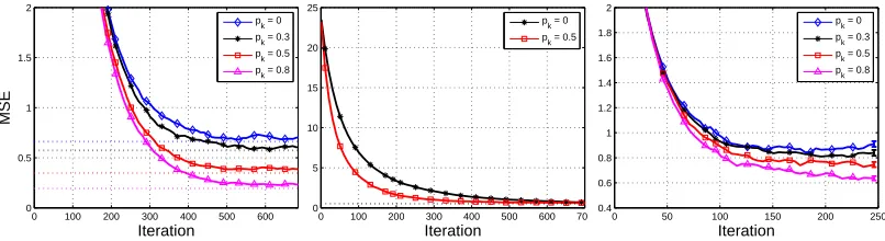
For aGARNET(10,5,10,1)MDP, a random deterministic policy was chosen and its value func-tion was evaluated using algorithm (17). The error kθK
n−θ∗k2, averaged over 500 different runs with the same initial conditions, is plotted in Figure 1 (left) for different values ofpK. The
asymp-totic MSE was calculated using (23) and is shown for comparison. In Figure 1 (middle), the step size for an iteration with partial knowledge was set such that the asymptotic MSE would match that of the iteration without partial knowledge. As can be seen, this caused the IPM iteration to converge
faster.
For the next simulation a linear FA was used, with basis vectors φ(x)∈ {0,1}L, where the number of nonzero values in eachφ(x)isl. The nonzero values were chosen uniformly at random, with any two states having different feature vectors. Figure 1 (right) shows the errorkθK
n−θ∗k
2
for aGARNET(30,5,10,1)MDP, where we used linear FA withL=10 andl=2. As can be seen, the
behavior observed in the tabular case is characteristic of the FA case as well.
5. Inaccuracy of the Partial Model
Until now, we have assumed that our partial model contained accurate probability ratios. Obviously, such a strong assumption is not realistic, and in any practical situation our partial knowledge would contain some degree of error. In this section we consider the effect of inaccuracies in the partial model on the performance of the IPM-TD(0) method. Specifically, our goal is to show that if the inaccuracy in the partially known model is small enough, then an improvement in performance over regular TD(0) can still be guaranteed, and we seek bounds on the error in the algorithm induced by the inaccuracy in the model. Before we go into mathematical detail we first describe our conceptual approach.
0 100 200 300 400 500 600 0
0.5 1 1.5 2
Iteration
MSE
p
k = 0
pk = 0.3 pk = 0.5 p
k = 0.8
0 100 200 300 400 500 600 700 0
5 10 15 20 25
Iteration
p
k = 0
pk = 0.5
0 50 100 150 200 250
0.4 0.6 0.8 1 1.2 1.4 1.6 1.8 2
Iteration
MSE
p
k = 0
pk = 0.3 pk = 0.5 p
k = 0.8
Figure 1: TD(0) with a Partial Model. Left : MSE of Table Based IPM-TD(0) on a GAR-NET(10,5,10,1) MDP with a deterministic random policy, for different values ofpK. Step
size isε=0.2. Dashed lines show the asymptotic MSE calculated by (23).Middle: MSE of Table Based IPM-TD(0) on a GARNET(10,5,10,1) MDP with a deterministic random policy. ForpK=0 (black-solid) a step sizeε=0.15 was used, and the asymptotic MSE
was calculated using (23) (black-dashed). ForpK=0.5 (red-solid) a step size was
calcu-lated (using (23)) such that its asymptotic MSE would equal that ofpK=0.Right: MSE
of linear FA IPM-TD(0) on a GARNET(30,5,10,1) MDP with a deterministic random policy, for different values of pK. Step size isε=0.15. The linear FA parameters are
L=10 andl=2. A discount factor ofγ=0.7 was used in all simulations. All results are averaged over 500 different runs with the same initial conditions. Error bars display the standard error of the mean; for clarity of presentation the bars are displayed only for the last iteration.
A key point in the analysis of IPM-TD(0) in Section 4 was that since the estimator ˆµK in (5) is
unbiased, then the ODE of the stochastic approximation does not change, and asymptotically the algorithm concentrates around its fixed point which is the true value function. This is no longer valid when the partial model is not accurate, as the inaccuracy induces a bias in ˆµK. Since we use
the estimator at every time step, this bias may accumulate, and the crucial question here is how it affects the algorithm asymptotically, and whether it can be guaranteed that small model errors do not cause a large deviation from the true value function.
The improvement in performance of IPM-TD(0) relied on the variance reduction property of ˆµK.
We shall see that if the inaccuracy in the partial model is small enough, then this property can still be guaranteed.
Thus, our analysis consists of investigating the bias and the variance of IPM-TD(0) with an inaccurate model. As we have done earlier, we first describe some results in the context of estimating the mean of a random variable, and later extend the results to the MDP setting.
5.1 Estimation of a Random Variable Mean
Consider the definitions of Section (2), and letPˆ(ω) ω∈Ωdenote inaccurate probabilities, obtained by some means. For someε>0 we define anε−known setKεby
Kε,ω:ω∈Ω s.t. PˆKε(ω)−PKε(ω)
where the probability measures ˆPKεandPKεare defined by ˆPKε(ω),Pˆ(ω)/ ∑
ω′∈Kε
ˆ
P(ω′)andP
Kε(ω),
P(ω)/ ∑ ω′∈Kε
P(ω′), respectively. Also denote by ˆE
Kε[·] and ˆVarKε[·]the expectation and variance
under the measure ˆPKε, and by EKε[·]and VarKε[·]the expectation and variance under the measure
PKε.
We motivate the definition of theε−known set with an example. Letxi ni=1denote i.i.d. sam-ples ofX. For some setK⊂Ωlet ˆPK(ω)denote the count ratios inK
ˆ
PK(ω) =
n ∑
i=1
1(xi=ω)
n
∑
i=1
1(xi∈K) forω∈K
0 else
,
where1 is the indicator function. It can be shown that ˆPK(ω) is an unbiased estimate of PK(ω),
and by the law of large numbers we have that for largen, the differencePˆK(ω)−PK(ω)
is small.
Furthermore, for a finite n, Chernoff type bounds can be used to bound this difference with high probability by some smallε, motivating definition (26).
An estimator forµthat uses theε−known set is derived by pluggingKεinstead ofKin (5)
ˆ
µKε(x) =1 Kε
x EˆKε[X] +1
¯
Kε
x x. (27)
Note that since the known set is not accurate, the estimator (27) is no longer unbiased. The following theorem, which we prove in Appendix C, bounds the bias and variance of ˆµKε(x).
Theorem 9 The bias of µˆKε(x)satisfies
|E[ˆµKε(X)]−E[X]| ≤εP(Kε)
∑
x∈Kε
|x|.
The variance of µˆKε(x)satisfies
Var[ˆµKε(X)] ≤ Var[X]−P(Kε)·VarKε[X] (28)
+εP(Kε)
ε
∑
x∈Kε
|x|
!2
+2
∑
x∈Kε
|x|
!
|EKε[X]−E[X]|
.
5.2 Error Bound for IPM-TD(0)
We now derive asymptotic error bounds for IPM-TD(0) with a constant stepsize ˜ε, when the partial model is inaccurate. We treat only the table based algorithm
θn+1(xn) = θn(xn) +˜εdnK, (29)
dK
n , r(xn) +γ
1Kε
n+1EˆKεxn[θn(xn+1)|xn] +1K¯ ε
n+1θn(xn+1)
−θn(xn),
where ˆEKεxn[θn(xn+1)|xn]denotes expectation under the probability measure in theε−known setKxεn
Kxε,
y:y∈
X
s.t.ˆ
P(y|x)
∑
y′∈Kεx
ˆ
P(y′|x)−
P(y|x)
∑
y′∈Kε
x
P(y′|x)
The ODE for (29) can be written as
dθ
dt =Π(r+ (γ(P+δP)−I)θ), (31)
where
δPi j=
∑
k∈Kεi
P(k|i)
!
ˆ
P(j|i)
∑
k∈Kεi
ˆ
P(k|i)−
P(j|i)
∑
k∈Kε i
P(k|i)
, j∈Kiε,
0, j∈/Kiε.
(32)
Recalling that the true value function satisfies θ∗= (I−γP)−1r, the asymptotic limit point of
the ODE (31) is denoted byθ∗+δθ, and satisfies
θ∗+δθ= (I−γ(P+δP))−1r. (33)
In the next subsection we show how to bound the error termδθ.
5.2.1 A BOUND ON THEBIAS
We would like to bound the termδθ, which is the error in the value function, and can be seen as the totalbias induced by the IPM method with the inaccurate model. Note that (33) describes a perturbed linear system (Horn and Johnson, 1985, §5). Using tools for dealing with such systems, we can bound the error as presented in the following theorem.
Theorem 10 Let Kmaxε denote the cardinality of the largestε−known set Kxε, Kmaxε =max
x |K
ε
x|, (34)
and letεsatisfyε<γ1K−εγ
max. Then the maximal error in the ODE limit is bounded by kδθk∞
kθ∗k ∞ ≤
κ
1−κ·Kmaxε ε
1−γ
Kmaxε ε
1−γ
, (35)
whereκsatisfies
κ≤1+γ
1−γ. (36)
Proof For a matrix normk·kp, if
(I−γP)
−1
pkγδPkp<1 we have (Horn and Johnson, 1985, 5.8.8)
kδθkp
kθ∗k
p
≤ κ(I−γP)
1−κ(I−γP)kγδPkp/kI−γPkp
kγδPkp
kI−γPkp, (37)
whereκis the matrix condition numberκ(A) = A−1
pkAkp. We now bound each of the terms on the right hand side of (37). We use the normk·k∞which is induced by the max vector norm, and can be alternatively defined (Horn and Johnson, 1985, 5.6.5) as themaximum row summatrix norm
kδPk∞,max
i
∑
jPi j
From this definition, (32), (34), and (30), it is clear that
kγδPk∞<γKmaxε ε. (39)
Theorem 5.6.9 in Horn and Johnson (1985) asserts that for any matrix norm we have
kAk ≥ρ(A),
whereρ(A)is the spectral radius ofA
ρ(A),max{|λ|:λis an eigenvalue ofA}.
For the matrixI−γPwe have
ρ(I−γP)>1−γ,
sincePis stochastic and thus its largest eigenvalue is 1. Using (39) we therefore have
kγδPk∞
kI−γPk∞≤
γKmaxε ε
1−γ .
We now boundκ(I−γP) =kI−γPk∞
(I−γP)
−1
∞. First, by the triangle equality we have
kI−γPk∞≤ kIk∞+γkPk∞=1+γ, (40)
sincePis a stochastic matrix and by definition (38) we havekPk∞=1. Next we have by definition
of the induced norm
(I−γP)
−1
∞=kmaxrk∞=1
(I−γP)
−1 r
∞≤
1
1−γ, (41)
since(I−γP)−1r can be seen as the value function associated with a reward vectorr, which can have a maximum value ofrmax/(1−γ). From (40) and (41) we have
κ(I−γP)≤ 1+γ 1−γ.
All is left is to verify that
(I−γP)
−1
∞kγδPk∞<1. Using (39) and (41) this is satisfied if ε< 1−γ
γKε max
.
The bound in (35) can be simplified whenεis small, as described in the following corollary.
Corollary 11 For small enoughεwe have
kδθk∞
kθ∗k ∞ ≤
Kmaxε ε(1+γ) (1−γ)2 +O ε
2 .
Proof Substitute (36) in (35), where for smallεwe haveε/1−κKmaxε ε
1−γ
=ε+O ε2
.
5.2.2 A BOUND ON THEVARIANCE
We shall now bound the variance of IPM-TD(0). We follow directly the analysis of Section 4 for IPM-TD(0) with an accurate model, and note that the only difference9 is in the calculation for the termΣKε
0 , which, using (33), becomes
h
ΣKε
0
i
xx = E
h
(dK
n)
2
θ=θ
∗+δθ,x
n=x
i
= γ2Varh 1Kε
n+1EˆKεxn[ [θ∗+δθ] (xn+1)|xn] +1K¯ ε
n+1[θ∗+δθ] (xn+1)
xn=x
i .
In the following we focus on bounding the term on the right hand side, and show sufficient condi-tions under whichΣKε
0
xx<[Σ0]xxfor everyx∈ |
X
|. For notational simplicity, we drop the depen-dence onx, and treat a single random variable taking values in{[θ∗+δθ]i}| X|
i=1, with the appropriate
probabilitiesP(x′|x). Thus, we need to bound
γ−2hΣKε
0
i
xx=Var
h
1Kεˆ
EKε[θ∗+δθ] +1
¯
Kε
(θ∗+δθ)i, (42)
and compare to[Σ0]xx. The following theorem, which is proved in Appendix D, boundsγ−2
ΣKε
0
xx.
Theorem 12 Let bx, ∑ x∈Kxε
|[θ∗]
x|, and cx,
EKεx[θ∗]−E[θ∗]
, and assume thatmax{δθ} ≤η. Then
the elements of the diagonal matrixΣK
0satisfy γ−2hΣKε
0
i
xx ≤ γ
−2[Σ
0]xx−P(K
ε
x)·VarKεx[θ∗] +η
2+2ηγ−1q[Σ 0]xx +εP(Kxε) εb2x(1−P(Kxε)) +2bxcx
. (43)
Using our previous bound on the bias we have the following corollary.
Corollary 13 For small enoughεwe have γ−2[Σ
0]xx−
h
ΣKε
0
i
xx
≥ P(Kxε)·VarKεx[θ∗]
−εK
ε
max(1+γ)kθ∗k∞
(1−γ)2
Kmaxε ε(1+γ)kθ∗k ∞
(1−γ)2 + 2
γ
q
[Σ0]xx
!
−εP(Kxε) εb2
x(1−P(Kxε)) +2bxcx
.
Proof Apply Corollary 11 to boundηin Theorem 12.
The following corollary translates the previously established bounds to a performance improvement guarantee.
Corollary 14 For a small enoughεan improvement in the asymptotic MSE of IPM-TD(0) can be guaranteed.
9. Note that theΣKε
Proof By Corollary 13εcan be chosen such that for everyxwe have
h
ΣKε
0
i
xx<[Σ0]xx,
thus we can follow the development of the performance improvement proof in Section 4 and conclude that the sequence (θK
n−θ∗)/
√
˜
ε converges in distribution to a Gaussian centered onδθ
and with a covariance ˆR, which is smaller than R (as defined in Section 4). Since we can use Theorem 10 to also bound the bias δθ, we can choose ε small enough such that asymptotically EkθK
n−θ∗k
2
<Ekθn−θ∗k2.
To conclude, from Theorem 10 and Theorem 12 we see that for small enoughε, we get a small bias and a reduction in the variance. The specific terms in the bounds can be used to find a suitableε
that guarantees a performance improvement. If the probabilities ˆPare obtained empirically from a trajectory of the MDP, then a Chernoff type bound can be used to further bound the number of observations required for a desiredε. This issue is beyond the scope of this paper.
6. Numerical Experiments
In this section, the performance improvement obtained by the IPM method is demonstrated on two different model free RL algorithms,10and two different problems. Our goal is to demonstrate both thegeneralityof the method, and itsusefulnessin practical applications. Generality is demonstrated by application of the method to two very different RL algorithms - policy gradient and Q-learning. The only common feature to these two algorithms is their representation as a stochastic approxi-mation. Together with the theory presented in previous sections, these results suggest that the IPM method can be applied succesfully to a wide variety of RL algorithms. The usefulness of the method is demonstrated in the solution of a call admission control problem. In this problem, it is shown that values of the partially known MDP (11) capture meaningful physical quantities of the problem, thus, (11) may be seen as the natural representation for partial knowledge in such problems. The performance improvement obtained by the IPM method suggests that it may be used succesfully in practice.
6.1 IPM Q-Learning for Admission Control
In this section we consider the call admission control problem for a single link, which arises when a telecommunication provider wants to sell the limited bandwidth of the link to different types of customers so as to maximize expected long term revenue. In this scenario, the customers differ in their bandwidth demand, the price they pay for its usage, and the frequency of their requests.
When the link is empty, it is reasonable that every customer request should be accepted, as it generates some revenue. On the other hand, when the link is almost full, a clever policy might decide to save the available bandwidth for the more profitable requests, at the expense of rejecting the less profitable ones. Thus, it is clear that a good policy should take into account both the bandwidth demand and profit of each request type, and its arrival frequency. When some of these quantities are not known in advance, alearning policy may be employed. Specifically, in the following we consider a case where these quantities are known only for someof the request types, which will naturally lead to the use of a partial model in the learning algorithm. Such a scenario can occur
when, for example, new customers are added to a system, or when some of the request types have features that change in time.11
One approach to designing an admission policy is to formulate the problem as an MDP, for which an optimal policy is well defined, and solve it using RL approaches, as has been done by Marbach et al. (1998) and Marbach and Tsitsiklis (1998). In the following we present this ap-proach, and show that in this problem our partially known MDP definition emerges as a very natural representation for partial model knowledge.
6.1.1 PROBLEMFORMULATION
Consider a service provider with a bandwidth ofBunits, which supports a finite set{1,2, ...,M}
of different service types. Each service type is characterized by its bandwidth demandb(m), its call arrival rateα(m), and its average holding time 1/β(m), where we assume that the calls arrive according to independent Poisson processes, and that the holding times are exponentially and inde-pendently distributed. Whenever a call of typemarrives, the controller can decide whether to accept or reject it, and if it is accepted and enough bandwidth is available, an immediate rewardc(m)is recieved. The objective is to find an admission controller (policy) that maximizes the average return. This problem can be represented by an MDP as follows.
6.1.2 STATESPACE, CONTROLS,ANDREWARD
The configuration of the link is denoted bys= (s(1), . . . ,s(M)), wheres(m)∈ {0,1,2, . . .}denotes the number of customers of typemcurrently using the link. Transitions between different configura-tions are triggered by events which we denote byω={ω(1), . . . ,ω(M)}, whereω(m) =1 if a new customer of typemrequests service,ω(m) =−1 if a customer of typemdeparts from the system, andω(m) =0 otherwise. The statexof the system consists of the link configuration together with the event which triggered a transition,
x= (s,ω),
and the complete state space is given by
X
=x= (s,ω)|
∑
s(m)b(m)≤B,∑
|ω(m)| ≤1 andω(m)<0 only if s(m)>0 .The possible controls are to accept or reject a call, denoted byu∈ {ua,ur}, respectively, and the immediate reward is
r(x,u) =
(
c(m) ifu=ua,ω(m) =1,(s+ω,ω)∈
X
,0 else.
The goal is to find the optimal policy with respect to the theaverage reward
η=E[r(x)].
6.1.3 TRANSITIONPROBABILITIES
In order to transform the continuous time process into discrete transitions between events, a uni-formization technique (Gallager, 1995, §6.4) is used. Define z to be the maximal transition rate, given by
z=max x∈X
(
M
∑
m=1(α(m) +s(m)β(m))
)
. (44)
For a statex= (s,ω), the probability that the next event is an arrival of a call of typemis equal to
α(m)/z. The probability for a departure of a call of typemisβ(m)s(m)/z. By normalization, the
probability that in the next event nothing happens is 1− M∑
m=1
(α(m) +s(m)β(m))/z.
6.1.4 PARTIALLYKNOWNMDP
For this problem, a natural definition for partial model knowledge is through the arrival and depar-ture ratesα,β, namely
MK,{m:m∈1, . . . ,Ms.t.α(m),β(m) are known}.
As an example where such partial knowledge arises in practice, consider a case where new jobs (with unknown rates) are added to an existing system (with previously known rates). Note that generally, the values inMKdo not suffice for calculatingzin (44), hence the transition probabilities
of the MDP are not known. Nevertheless, the key point here is that in theratiosbetween transition probabilities, thezterms cancel out, therefore the partial MDP definition (11) can be satisfied. In particular, lettingi∈MK, we have
P(arrival of typei)
∑
j∈MK
P(arrival of type j) =
α(i)
∑
j∈MK
α(j),
and similar expressions hold for probabilities of departures.
6.1.5 IPM Q-LEARNING
The model free RL algorithm we use for this problem is a variant of the popular Q-Learning al-gorithm for average return.12 For each state-action pair, a Q value is maintained, and updated according to
Qn+1(xn,un) =Qn(xn,un) +εn r(xn,un) +max
u′ Qn xn+1,u
′
−Qn(xn,un)− 1
|
X
||U
|∑
x,u
Qn(x,u)
!
.
(45) The greedy deterministic policyu(x)w.r.t. theQvalues at timenis
u(x) =argmax u′
Qn x,u′
.
Update (45) is an SA, and was shown to converge (Abounadi et al., 2001) under suitable step sizes
εnto a fixed pointQ∗, such that the greedy policy w.r.t.Q∗is optimal. Applying the IPM method in
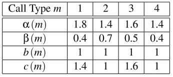
Call Typem 1 2 3 4
α(m) 1.8 1.4 1.6 1.4
β(m) 0.4 0.7 0.5 0.4
b(m) 1 1 1 1
c(m) 1.4 1 1.6 1
Table 1: Call Types
this case simply amounts to replacing max
u′ Qn(xn+1,u
′)in (45) with
1K
n+1· ∑
y∈Kxn,un
Pun(y|xn)max
u′ Qn(y,u
′) ∑
y∈Kxn,un
Pun(y|xn)
+1K¯
n+1·max
u′ Qn xn+1,u
′
. (46)
We now report on the results of using IPM Q-learning for optimizing a call admission control policy.
6.1.6 RESULTS
In our experiments, we consider a link with a bandwidth of 7 units, and 4 call types. The parameters for each call are summarized in Table 1, and the size of the state space in this configuration is
|
X
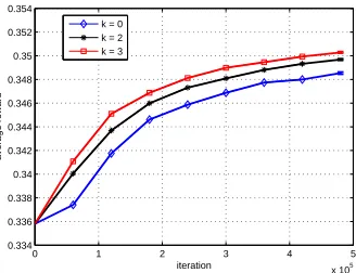
|=2490. IPM Q-Learning was run with initial values Q0(x,u) =r(x,u) and a step sizeεn= γ0/(γ1+vn(xn,un)),wherevn(x,u)denotes the number of visits to the state action pair(x,u)up to timen. The values ofγ0,γ1were manually tuned for optimal performance, and set toγ0=γ1=40.The action selection policy while learning wasε−greedy,withε=0.1. The partial model for each experiment is represented by a single parameterk, such that the arrival and departure rates of all calls of typem≤kare known. Figure 2 shows the average rewardηas a function of iteration. As can be seen, incorporation of partial model knowledge by the IPM method resulted in a significant performance improvement.
6.2 IPM Policy Gradient
In this experiment simulations were performed on randomly generated MDP’s, as described in Section 4.3. In the experiments, the agent maintains a stochastic policy function parametrized by
θ∈RL·|U|, and given by
µθ(u|x) =eθ
Tξ(x,u)
/
∑
u′
eθTξ(x,u′),
where the state-action feature vectors ξ(x,u)∈ {0,1}L·|U| are constructed from the state features
φ(x)defined in Section 4.3 as follows
ξ(x,u),(0, ...(L×(u−1)zeros),φ(x),0, ...(L×(|
U
| −u)zeros))T.The agent’s goal is to find the parameterθwhich maximizes theaverage rewardη=E[r(x)].Policy Gradient algorithms achieve this goal by estimating the gradient w.r.t.θof the average reward,∇θη,
and performing a stochastic gradient ascent on the parameters to reach a local maximum. One such algorithm was proposed by Marbach and Tsitsiklis (1998). At timenwe update the parameter vector
0 1 2 3 4 5 x 10⁵ 0.334
0.336 0.338 0.34 0.342 0.344 0.346 0.348 0.35 0.352 0.354
iteration
average reward
k = 0 k = 2 k = 3
Figure 2: IPM Q-Learning for Admission control. Implementation of IPM Q-Learning, (45) and (46), for the call admission control problem of Table 1. Average reward of the greedy policy is plotted vs. iteration number for different values ofk. Results are averaged over 100 different runs with the same initial conditions. Error bars display the standard error of the mean; for clarity of presentation the bars are displayed only for the last iteration.
θn+1 = θn+ε(r(xn)−λn)zn, (47)
λn+1 = λn+ε′(r(xn)−λn), (48)
whereεandε′are step sizes, andε′<ε. We then simulate a transition to the next state, and update the vectorzby
zn+1=zn+Lxn,un(θn),
whereLxn,un(θn)is the likelihood ratioLx,u(θ) =∇θlogµθ(u|x). Every time a predefined recurrent
state of the MDP is visited,zn+1is reset to zero.
Denote by 1K
n an indicator function that equals 1 if xn belongs to Kxn−1,un−1 and 0 otherwise.
Incorporating partial knowledge into the algorithm using (12) simply amounts to replacingr(xn)in (47-48) with
1K
n·
∑
y∈Kxn−1,un−1
Pun−1(y|xn−1)r(y)
∑
y∈Kxn−1,un−1
Pun−1(y|xn−1)
+1K¯
n·r(xn).
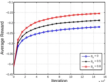
We simulated the policy gradient algorithm on aGARNET(30,5,10,1)MDP. The state features
were constructed as described in Section 4.3 withL=10,l=2. Figure 3 shows the average reward
η as a function of iteration. These results indicate that the variance reduction in each iteration (guaranteed by Lemma 2) resulted, on average, in a better estimation of the gradient ∇θη, and
therefore a better policy at each step.
7. Discussion and Future Work
0 2 4 6 8 10 12 14 16 x 104
−0.45 −0.4 −0.35 −0.3 −0.25 −0.2 −0.15 −0.1
Iteration
Average Reward
p
k = 0
pk = 0.5 p
k = 0.8
Figure 3: Policy Gradient with a Partial Model. Implementation of the algorithm described in Section 6.2 on a GARNET(30,5,10,1) MDP, with step size parameters ε =0.03 and
ε′=0.003. The linear FA parameters areL=10 andl=2. Average reward is plotted vs. iteration number for different values of pK. Results are averaged over 500 different
runs with the same initial conditions. Error bars display the standard error of the mean; for clarity of presentation the bars are displayed only for the last iteration.
the underlying environment, and therefore, when such knowledge is available, using these algo-rithms ‘out of the box’ is clearly suboptimal. In this work we have presented a general method of integrating partial environmental knowledge into a large class of model free algorithms. Our method improves the asymptotic behavior of the algorithm, and at each iteration reduces the esti-mation variance due to the uncertainty in the environment. We have proved mathematically (for TD(0)) and demonstrated in simulation (for Policy Gradient and Q-learning) an improvement in the algorithm’s overall performance.
From a more conceptual point of view, we have shown that two distinct approaches to RL, the model free and the model based approaches, can be combined in such a way that gains from their respective merits. From this perspective, this work is just a first step towards a theoretical understanding of the combination of different RL approaches.
A few issues are in need of further investigation.
In this work we have not addressed the question of how the partially known model can be acquired. A number of possibilities come to mind. In a transfer learning or tutor learning settings, the partial model can come from an expert who has exact knowledge of a model that is partially similar. In a multi-agent setting with communication, information about different parts of the model can be gathered independently by each of the agents, and combined to create a partial model of the environment.
meanm, and assume that our goal is to estimatem. A natural approach is to use the empirical mean given byθn=1n∑ni=1xi, which can also be calculated recursively using the following SA iterate
θn+1 = θn+ 1
n+1(xn+1−θn), (49)
θ0 = 0.
One may hope, that by the time of then’th update ofθwe could use then−1 values ofxi already observed to build a partial model forxn, and similarly to (12), use it to manipulate (49) in such a way that guarantees a performance improvement (in the estimation of m). However, it is known that for a normal distribution, the empirical mean is also the minimum variance unbiased estimator form(Schervish, 1995). Our manipulation of (49) would therefore either add bias or increase the variance. Though this issue deserves careful analysis, we note that when a constant step size is used, the major influences on the current value of the parameter are the most recent measurements, thus older samples can be safely used to construct a partial model, mitigating the severity of this problem.
Finally, we note that the IPM method adds to the algorithm a computational cost of O(Kmax)
evaluations ofF(θn,xn,un,xn+1)at each iteration. In our experiments, this cost proved to be
neg-ligible in comparison to the computational cost of the simulator. However, if the computation of
F(θn,xn,un,xn+1)is demanding, one may face a tradeoff between the performance of the resulting
policy and the computational cost of obtaining it.
Acknowledgments
The authors would like to thank Nahum Shimkin for helpful discussions.
Appendix A. Admissibility ofµˆK
In this section, based on the definitions of Section 2, we address the following issue. Can a better estimator than ˆµK(x)be found?
Since the MSE of any estimator, within a non-Bayesian setting, depends on the unknown µ, comparison of different estimators is a difficult task. A popular comparison framework is that ofadmissible estimators (Schervish, 1995). For a given known set K, an estimator is said to be admissible if there is no other estimator that achieves a smaller MSE for every distribution in
P
K(ω).Clearly, admissibility is a desirable property for an estimator, since an inadmissible estimator is guaranteed to be sub-optimal. The next theorem states that ˆµKis admissible.
Theorem 15 The estimatorµˆKof (5)is admissible.
Proof Let ˜P(ω)∈
P
K(ω)be defined as˜
P(ω) = 1
K
ωP(ω) ∑ ω′∈KP(ω
′).
For X ∼P˜(ω) it is clear that ˆµK(x) =E[X]for all x, therefore E[ˆµK(X)−µ]
2
Appendix B. Proof of Lemma 5
Proof By the ergodicity of the Markov chain the joint probability for subsequent states is lim
n→∞P(xn,xn+1) = P(xn+1|xn) [π]xn.
Now, observe that
Eh(dnφ(xn)) (dnφ(xn))T
θn=θ
∗,x
n
i
=Cov[dnφ(xn)|θn=θ∗,xn] +E[ (dnφ(xn))|θn=θ∗,xn]E[ (dnφ(xn))|θn=θ∗,xn]T =γ2φ(xn)Covφ(xn+1)Tθ∗
xn
φ(xn)T
+E[dnφ(xn)|θn=θ∗,xn]E[dnφ(xn)|θn=θ∗,xn]T, where the second equality follows from
Cov[dnφ(xn)|θn,xn] =Cov
dnφ(xn)−r(xn) +φ(xn)Tθn
θn,xn
,
since adding constants does not change the covariance. Using Lemma 1 and Lemma 2 we derive an expression for the IPM iteration
Eh(dK
nφ(xn)) (dKnφ(xn))T
θn=θ
∗,x
n
i
=γ2φ(x
n) Cov
φ(xn+1)Tθ∗
xn
−P(Kx)CovK
φ(xn+1)Tθ∗
xn
φ(xn)T +E[dK
nφ(xn)|θn=θ∗,xn]E[dnKφ(xn)|θn=θ∗,xn]T =E
h
(dnφ(xn)) (dnφ(xn))T
θn=θ
∗,x
n
i
−γ2φ(xn)P(Kx)CovK
φ(xn+1)Tθ∗
xn
φ(xn)T.
We therefore have that
Σ0 = lim
n→∞E
h
(dnφ(xn)) (dnφ(xn))T
θn=θ
∗i
= lim
n→∞E
h
E
h
(dnφ(xn)) (dnφ(xn))T
θn=θ
∗,x
n
ii
=
∑
x
[π]xEh(dnφ(xn)) (dnφ(xn))T
θn=θ
∗,x
n
i
= ΣK
0+γ2
∑
x
[π]xφ(x)P(Kx)CovK
φ(x′)Tθ∗ x
φ(x)T
= ΣK
0+γ2
∑
x
[π]xφ(x)P(Kx)VarK
φ(x′)Tθ∗ x
φ(x)T.
Appendix C. Proof of Theorem 9
Proof First, observe that
EˆKε[X]−EKε[X]
=
∑
x∈Kεx PˆKε(x)−PKε(x)
≤ε
∑
x∈Kε