Greedy Feature Selection for Subspace Clustering

Greedy Feature Selection for Subspace Clustering

Eva L. Dyer [email protected]

Department of Electrical & Computer Engineering Rice University

Houston, TX, 77005, USA

Aswin C. Sankaranarayanan [email protected]

Department of Electrical & Computer Engineering Carnegie Mellon University

Pittsburgh, PA, 15213, USA

Richard G. Baraniuk [email protected]

Department of Electrical & Computer Engineering Rice University

Houston, TX, 77005, USA

Editor:Tong Zhang

Abstract

Unions of subspaces provide a powerful generalization of single subspace models for collections of high-dimensional data; however, learning multiple subspaces from data is challenging due to the fact that segmentation—the identification of points that live in the same subspace—and subspace estimation must be performed simultaneously. Recently, sparse recovery methods were shown to provide a provable and robust strategy forexact feature selection(EFS)—recovering subsets of points from the ensemble that live in the same subspace. In parallel with recent studies of EFS withℓ1-minimization, in this paper, we develop sufficient conditions for EFS with a greedy method for sparse signal recovery known as orthogonal matching pursuit (OMP). Following our analysis, we provide an empirical study of feature selection strategies for signals living on unions of sub-spaces and characterize the gap between sparse recovery methods and nearest neighbor (NN)-based approaches. In particular, we demonstrate that sparse recovery methods provide significant advan-tages over NN methods and that the gap between the two approaches is particularly pronounced when the sampling of subspaces in the data set is sparse. Our results suggest that OMP may be employed to reliably recover exact feature sets in a number of regimes where NN approaches fail to reveal the subspace membership of points in the ensemble.

Keywords: subspace clustering, unions of subspaces, hybrid linear models, sparse approximation, structured sparsity, nearest neighbors, low-rank approximation

1. Introduction

With the emergence of novel sensing systems capable of acquiring data at scales ranging from the nano to the peta, modern sensor and imaging data are becoming increasingly high-dimensional and heterogeneous. To cope with this explosion of high-dimensional data, one must exploit the fact that low-dimensional geometric structure exists amongst collections of data.

com-putational sciences. This is due in part to the simplicity of linear models but also due to the fact that principal components analysis (PCA) provides a closed-form and computationally efficient solution to the problem of finding an optimal low-rank approximation to a collection of data (an ensemble of signals inRn_{). More formally, if we stack a collection ofd vectors (points) inR}n_{into the columns} ofY _∈Rn×d_{, then PCA finds the best rank-kestimate ofY by solving}

(PCA) min

X∈Rn×d

n

∑

i=1 d

∑

j=1

(Yi j−Xi j)2 subject to rank(X)≤k, (1)

whereXi jis the(i,j)entry ofX.

1.1 Unions of Subspaces

In many cases, a linear subspace model is sufficient to characterize the intrinsic structure of an ensemble; however, in many emerging applications, a single subspace is not enough. Instead, en-sembles can be modeled as living on aunion of subspacesor a union of affine planes of mixed or equal dimension. Formally, we say that a set ofd signals

Y

=_{y1, . . . ,yd}, each of dimensionn, lives on a union ofpsubspaces if

Y

_⊂

U

=_∪ip₌₁

S

i,where

S

iis a subspace ofRn.

Ensembles ranging from collections of images taken of objects under different illumination con-ditions (Basri and Jacobs, 2003; Ramamoorthi, 2002), motion trajectories of point-correspondences (Kanatani, 2001), to structured sparse and block-sparse signals (Lu and Do, 2008; Blumensath and Davies, 2009; Baraniuk et al., 2010) are all well-approximated by a union of low-dimensional sub-spaces or a union of affine hyperplanes. Union of subspace models have also found utility in the classification of signals collected from complex and adaptive systems at different instances in time, for example, electrical signals collected from the brain’s motor cortex (Gowreesunker et al., 2011).

1.2 Exact Feature Selection

Unions of subspaces provide a natural extension to single subspace models, but providing an ex-tension of PCA that leads to provable guarantees for learning multiple subspaces is challenging. This is due to the fact thatsubspace clustering—the identification of points that live in the same subspace—and subspace estimation must be performed simultaneously. However, if we can sift through the points in the ensemble and identify subsets of points that lie along or near the same sub-space, then alocal subspace estimate1formed from any such set is guaranteed to coincide with one of the true subspaces present in the ensemble (Vidal et al., 2005; Vidal, 2011). Thus, to guarantee that we obtain an accurate estimate of the subspaces present in a collection of data, we must select a sufficient number of subsets (feature sets) containing points that lie along the same subspace; when a feature set contains points from the same subspace, we say that exact feature selection (EFS) occurs.

A common heuristic used for feature selection is to simply select subsets of points that lie within an Euclidean neighborhood of one another (or a fixed number of nearest neighbors (NNs)). Methods that use sets of NNs to learn a union of subspaces include: local subspace affinity (LSA) (Yan and Pollefeys, 2006), spectral clustering based on locally linear approximations (Arias-Castro et al., 2011), spectral curvature clustering (Chen and Lerman, 2009), and local best-fit flats (Zhang et al.,

2012). When the subspaces present in the ensemble are non-intersecting and densely sampled, NN-based approaches provide high rates of EFS and in turn, provide accurate local estimates of the subspaces present in the ensemble. However, such approaches quickly fail as the intersection between pairs of subspaces increases and as the number of points in each subspace decreases; in both of these cases, the Euclidean distance between points becomes a poor predictor of whether points belong to the same subspace.

1.3 Endogenous Sparse Recovery

Instead of computing local subspace estimates from sets of NNs, Elhamifar and Vidal (2009) pro-pose a novel approach for feature selection based upon forming sparse representations of the data viaℓ1-minimization. The main intuition underlying their approach is that when a sparse represen-tation of a point is formed with respect to the remaining points in the ensemble, the represenrepresen-tation should only consist of other points that belong to the same subspace. Under certain assumptions on both the sampling and “distance between subspaces”,2this approach to feature selection leads to provable guarantees that EFS will occur, even when the subspaces intersect (Elhamifar and Vidal, 2010; Soltanolkotabi and Cand`es, 2012).

We refer to this application of sparse recovery as endogenous sparse recovery due to the fact that representations are not formed from an external collection of primitives (such as a basis or dictionary) but are formed “from within” the data. Formally, for a set ofdsignals

Y

=_{y1, . . . ,yd}, each of dimensionn, the sparsest representation of theithpointyi∈Rnis defined as

c∗_i = arg min

c∈Rd kck0 subject to yi=

∑

j₆=i

c(j)yj, (2)

where_kc_k0counts the number of non-zeroes in its argument andc(j)∈Rdenotes the contribution of the jthpointyjto the representation ofyi. LetΛ(i)=supp(c∗i)denote the subset of points selected to represent theithpoint andc∗_i(j)denote the contribution of the jth point to the endogenous repre-sentation ofyi. By penalizing representations that require a large number of non-zero coefficients, the resulting representation will be sparse.

In general, finding the sparsest representation of a signal has combinatorial complexity; thus, sparse recovery methods such as basis pursuit (BP) (Chen et al., 1998) or low-complexity greedy methods (Davis et al., 1994) are employed to obtain approximate solutions to (2).

1.4 Contributions

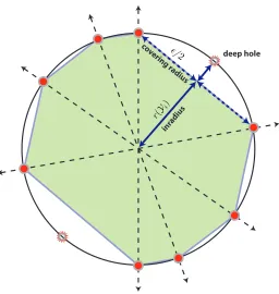
In parallel with recent studies of feature selection withℓ1-minimization (Elhamifar and Vidal, 2010; Soltanolkotabi and Cand`es, 2012; Elhamifar and Vidal, 2013), in this paper, we study feature selec-tion with a greedy method for sparse signal recovery known as orthogonal matching pursuit (OMP). The main result of our analysis is a new geometric condition (Theorem 1) for EFS with OMP that highlights the tradeoff between the: mutual coherenceor similarity between points living in differ-ent subspaces and thecovering radiusof the points within the same subspace. The covering radius can be interpreted as the radius of the largest ball that can be embedded within each subspace with-out touching a point in the ensemble; the vector that lies at the center of this open ball, or the vector in the subspace that attains the covering radius is referred to as adeep hole. Theorem 1 suggests that

r(

Yi)

co_{vering r}

adius

inradius

deep hole

Figure 1: Covering radius of points in a normalized subspace. The interior of the antipodal convex hull of points in a normalized subspace—a subspace ofRn_{mapped to the unitℓ2-sphere—} is shaded. The vector in the normalized subspace (unit circle) that attains the covering radius (deep hole) is marked with a star: when compared with the convex hull, the deep hole coincides with the maximal gap between the convex hull and the set of all vectors that live in the normalized subspace.

subspaces can be arbitrarily close to one another and even intersect, as long as the data is distributed “nicely” along each subspace. By “nicely”, we mean that the points that lie on each subspace do not cluster together, leaving large gaps in the sampling of the underlying subspace. In Figure 1, we illustrate the covering radius of a set of points on the sphere (the deep hole is denoted by a star).

After introducing a general geometric condition for EFS, we extend this analysis to the case where the data live on what we refer to as abounded union of subspaces(Theorem 3). In particular, we show that when the points living in a particular subspace are incoherent with the principal vec-tors that support pairs of subspaces in the ensemble, EFS can be guaranteed, even when non-trivial intersections exist between subspaces in the ensemble. Our condition for bounded subspaces sug-gests that, in addition to properties related to the sampling of subspaces, one can characterize the separability of pairs of subspaces by examining the correlation between the data set and the unique set of principal vectors that support pairs of subspaces in the ensemble.

we observe that while OMP, BP, and NN provide comparable rates of EFS when subspaces in the ensemble are non-intersecting and densely sampled, sparse recovery methods provide significantly higher rates of EFS than NN sets when: (i) the dimension of the intersection between subspaces increases and (ii) the sampling density decreases (fewer points per subspace). In Section 5.4, we study the performance of OMP, BP, and NN-based subspace clustering on real data, where the goal is to cluster a collection of images into their respective illumination subspaces. We show that clustering the data with OMP-based feature selection (see Algorithm 2) provides improvements over NN and BP-based (Elhamifar and Vidal, 2010, 2013) clustering methods. In the case of very sparsely sampled subspaces, where the subspace dimension equals 5 and the number of points per subspace equals 16, we obtain a 10% and 30% improvement in classification accuracy with OMP (90%), when compared with BP (80%) and NN (60%).

1.5 Paper Organization

We now provide a roadmap for the rest of the paper.

Section 2.We introduce a signal model for unions of subspaces, detail the sparse subspace clustering (SSC) algorithm (Elhamifar and Vidal, 2010), and then go on to introduce the use of OMP for feature selection and subspace clustering (Algorithm 2); we end with a motivating example.

Section 3 and 4.We provide a formal definition of EFS and then develop the main theoretical results of this paper. We introduce sufficient conditions for EFS to occur with OMP for general unions of subspaces in Theorem 1, disjoint unions in Corollary 1, and bounded unions in Theorem 3.

Section 5.We conduct a number of numerical experiments to validate our theory and compare sparse recovery methods (OMP and BP) with NN-based feature selection. Experiments are provided for both synthetic and real data.

Section 6. We discuss the implications of our theoretical analysis and empirical results on sparse approximation, dictionary learning, and compressive sensing. We conclude with a number of inter-esting open questions and future lines of research.

Section 7.We supply the proofs of the results contained in Sections 3 and 4.

1.6 Notation

In this paper, we will work solely in real finite-dimensional vector spaces,Rn_{. We write vectorsxin} lowercase script, matricesAin uppercase script, and scalar entries of vectors asx(j). The standard p-norm is defined as

kx_kp=

_n

∑

j=1

|x(j)_|p 1/p

,

where p_≥1. The “ℓ0-norm” of a vector x is defined as the number of non-zero elements in x. The support of a vectorx, often written as supp(x), is the set containing the indices of its non-zero coefficients; hence, _kx_k0=|supp(x)|. We denote the Moore-Penrose pseudoinverse of a matrixA asA†. IfA=UΣVT thenA†=VΣ+UT, where we obtainΣ+ by taking the reciprocal of the entries inΣ, leaving the zeros in their places, and taking the transpose. An orthonormal basis (ONB) Φ

that spans the subspace

S

of dimension k satisfies the following two properties: ΦT_{Φ =I} k and range(Φ) =

S

, whereIkis thek×kidentity matrix. LetPΛ=XΛX_Λ†denote an ortho-projector onto

2. Sparse Feature Selection for Subspace Clustering

In this section, we introduce a signal model for unions of subspaces, detail the sparse subspace clustering (SSC) method (Elhamifar and Vidal, 2009), and introduce an OMP-based method for sparse subspace clustering (SSC-OMP).

2.1 Signal Model

Given a set of p subspaces of Rn_{, {}

S

₁, . . . ,

S

_p}, we generate a “subspace cluster” by samplingdi points from theithsubspace

S

_iof dimensionki≤k. Let

Y

eidenote the set of points in theithsubspace cluster and let

Y

e =_∪ip₌₁

Y

e_idenote the union of psubspace clusters. Each point in

Y

e is mapped to the unit sphere to generate a union of normalized subspace clusters. Let

Y

=

y1

ky1k2 , y2

ky2k2

,_···, yd

kydk2

denote the resulting set of unit norm points and let

Y

_ibe the set of unit norm points that lie in the span of subspace

S

i. Let

Y

₋i=

Y

\

Y

i denote the set of points in

Y

with the points in

Y

iexcluded.

LetY = [Y1Y2 ··· Yp]denote the matrix of normalized data, where each point in

Y

iis stacked into the columns ofYi∈Rn×di. The points inYican be expanded in terms of an ONBΦi∈Rn×kithat spans

S

_iand subspace coefficientsAi=ΦTiYi, whereYi=ΦiAi. LetY−idenote the matrix containing the points inY with the sub-matrixYiexcluded.

2.2 Sparse Subspace Clustering

The sparse subspace clustering (SSC) algorithm (Elhamifar and Vidal, 2009) proceeds by solving the following basis pursuit (BP) problem for each point in

Y

:

c∗_i = arg min

c∈Rd kck1 subject to yi=

∑

j6=i

c(j)yj.

After solving BP for each point in the ensemble, eachd-dimensional feature vectorc∗_i is placed into theithrow or column of a matrixC∈Rd×d and spectral clustering (Shi and Malik, 2000; Ng et al., 2002) is performed on the graph Laplacian of the affinity matrixW=_|C_|+_|CT_|.

In situations where points might not admit an exact representation with respect to other points in the ensemble, an inequality constrained version of BP known as basis pursuit denoising (BPDN) may be employed for feature selection (Elhamifar and Vidal, 2013). In this case, the following BPDN problem is computed for each point in

Y

:

c∗_i = arg min

c∈Rd kck1 subject to kyi−

∑

j6=i

c(j)yjk2<κ, (3)

Algorithm 1:Orthogonal Matching Pursuit (OMP)

Input:Input signaly_∈Rn_{, a matrixA∈}Rn×d_{containingdsignals{ai}}d_i

=1in its columns, and a stopping criterion (either the sparsitykor the approximation errorκ).

Output:An index setΛcontaining the indices of all atoms selected in the pursuit and a coefficient vectorccontaining the coefficients associated with of all atoms selected in the pursuit.

Initialize: Set the residual to the input signals=y.

1. Select the atom that is maximally correlated with the residual and add it toΛ

Λ_←Λ _∪ arg max

i |hai,si|.

2. Update the residual by projectingsinto the space orthogonal to the span ofAΛ

s_←(I₋PΛ)y.

3. Repeat steps (1)–(2) until the stopping criterion is reached, for example, either_|Λ_|=k or the norm of the residual_ks_k2≤κ.

4. Return the support setΛand coefficient vectorc=A†_Λy.

2.3 Greedy Feature Selection

Instead of solving the sparse recovery problem in (2) viaℓ1-minimization, we propose the use of a low-complexity method for sparse recovery known as orthogonal matching pursuit (OMP). We detail the OMP algorithm in Algorithm 1. For each point yi, we solve Algorithm 1 to obtain a sparse representation of the signal with respect to the remaining points inY. The output of the OMP algorithm is a feature set, Λ(i)_{, which indexes the columns inY selected to form an endogenous}

representation ofyi.

After computing feature sets for each point in the data set via OMP, either a spectral clustering method or a consensus-based method (Dyer, 2011) may then be employed to cluster the data. In Algorithm 2, we outline a procedure for performing an OMP-based variant of the SSC algorithm that we will refer to as SSC-OMP.

2.4 Motivating Example: Clustering Illumination Subspaces

Algorithm 2:Sparse Subspace Clustering with OMP (SSC-OMP) Input: A data setY _∈Rn×d _{containingd points{yi}}d_i

=1 in its columns, a stopping criterion for OMP, and the number of clusters p.

Output: A set of d labels

L

=_{ℓ(1), ℓ(2), . . . , ℓ(d)_}, where ℓ(i) _{∈ {}1,2, . . . ,p_} is the label associated with theithpointyi.

Step 1. Compute Subspace Affinity via OMP

1. Solve Algorithm 1 for theith pointyito obtain a feature setΛand coefficient vectorc. 2. For all j_∈Λ(i)_{, letC}

i j =c(j). Otherwise, setCi j=0. 3. Repeat steps (1)–(2) for alli=1, . . . ,d.

Step 2. Perform Spectral Clustering

1. Symmetrize the subspace affinity matrixCto obtainW=_|C_|+_|CT_|. 2. Perform spectral clustering onW to obtain a set ofdlabels

L

.

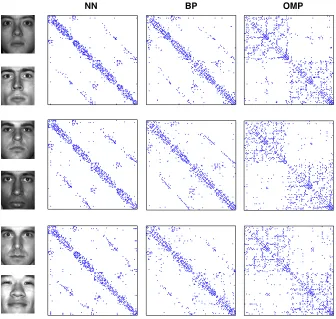
To generate the OMP affinity matrices in the right column, we use the greedy feature selection procedure outlined in Step 1 of Algorithm 2, where the sparsity level k=5. To generate the BP affinity matrices in the middle column, we solved the BPDN problem in (3) via a homotopy algo-rithm where we vary the noise parameterκand choose the smallest value ofκthat produces up to 5 coefficients. The resulting coefficient vectors are then stacked into the rows of a matrixCand the final subspace affinityW is computed by symmetrizing the coefficient matrix,W =_|C_|+_|CT_|. To generate the NN affinity matrices in the left column, we compute the absolute normalized inner products between all points in the data set and then threshold each row to select thek=5 nearest neighbors to each point.

3. Geometric Analysis of Exact Feature Selection

In this section, we provide a formal definition of EFS and develop sufficient conditions that guaran-tee that EFS will occur for all of the points contained within a particular subspace cluster.

3.1 Exact Feature Selection

In order to guarantee that OMP returns a feature set (subset of points from

Y

) that produces an accurate local subspace estimate, we will be interested in determining when the feature set returned by Algorithm 1 only contains points that belong to the same subspace cluster, that is,exact feature selection(EFS) occurs. EFS provides a natural condition for studying performance of both subspace consensus and spectral clustering methods due to the fact that when EFS occurs, this results in a local subspace estimate that coincides with one of the true subspaces contained within the data. We now supply a formal definition of EFS.

Definition 1 (Exact Feature Selection) Let

Y

_k=_{y:(I₋Pk)y=0,y∈

Y

}index the set of points

in

Y

that live in the span of subspace

S

_k, where Pk is a projector onto the span of subspace

S

k. For

NN BP OMP

Figure 2: Comparison of subspace affinity matrices for illumination subspaces. In each row, we display the affinity matrices obtained for a different pair of illumination subspaces, for NN (left), BP (middle), and OMP (right). To the left of the affinity matrices, we display an exemplar image from each illumination subspace.

3.2 Sufficient Conditions for EFS

In this section, we develop geometric conditions that are sufficient for EFS with OMP. Before pro-ceeding, however, we must introduce properties of the data set required to develop our main results.

3.2.1 PRELIMINARIES

Our main geometric result in Theorem 1 below requires measures of both the distance between points indifferent subspace clustersand within thesame subspace cluster. A natural measure of the similarity between points living in different subspaces is themutual coherence. A formal definition of the mutual coherence is provided below in Def. 2.

Definition 2 (Mutual Coherence)The mutual coherence between the points in the sets(Yi,

Y

j)is

defined as

µc(Yi,

Y

j) = max u∈Yi,v∈Yj

In words, the mutual coherence provides a point-wise measure of the normalized inner product (coherence) between all pairs of points that lie in two different subspace clusters.

Letµc(Yi)denote the maximum mutual coherence between the points in

Y

i and all other sub-space clusters in the ensemble, where

µc(Yi) =max

j₆=i µc(Yi,

Y

j).

A related quantity that provides an upper bound on the mutual coherence is the cosine of the firstprincipal anglebetween the subspaces. The first principal angleθ∗_{i j} between subspaces

S

iand

S

_j, is the smallest angle between a pair of unit vectors(u1,v1)drawn from

S

i×

S

j. Formally, the first principal angle is defined as

θ∗_{i j}= min u∈Si,v∈Sj

arccos_hu,v_i subject to _ku_k2=1,kvk2=1. (4) Whereas the mutual coherence provides a measure of the similarity between a pair of unit norm vectors that are contained in the sets

Y

_iand

Y

_j, the cosine of the minimum principal angle provides a measure of the similarity between all pairs of unit norm vectors that lie in the span of

S

i×

S

j. For this reason, the cosine of the first principal angle provides an upper bound on the mutual coherence. The following upper bound is in effect for each pair of subspace clusters in the ensemble:

µc(Yi,

Y

j)≤cos(θ∗i j). (5)

To measure how well points in the same subspace cluster cover the subspace they live on, we will study the covering radius of each normalized subspace cluster relative to the projective distance. Formally, the covering radius of the set

Y

_k is defined as

cover(Yk) = max u∈Sk

min y_∈Yk

dist(u,y),

where the projective distance between two vectors u andy is defined relative to the acute angle between the vectors

dist(u,y) = s

1₋ |hu,yi| 2

ku_k2kyk2 .

The covering radius of the normalized subspace cluster

Y

_i can be interpreted as the size of the largest open ball that can be placed in the set of all unit norm vectors that lie in the span of

S

i, without touching a point in

Y

_i.

Let (u∗_i,y∗_i) denote a pair of points that attain the maximum covering diameter for

Y

_i; u∗_i is referred to as a deep hole in

Y

i along

S

i. The covering radius can be interpreted as the sine of the angle between the deep holeu∗_{i ∈}

S

_i and its nearest neighbory∗_{i ∈}

Y

_i. We show the geometry underlying the covering radius in Figure 1.

In the sequel, we will be interested in the maximum (worst-case) covering attained over all di sets formed by removing a single point from

Y

_i. We supply a formal definition below in Def. 3.

Definition 3 (Covering Radius)The maximum covering diameterεof the set

Y

_ialong the subspace

S

_i is defined as

ε = max j=1,...,di

2 cover(_{

Y

i\yj}).

A related quantity is theinradiusof the set

Y

_i, or the cosine of the angle between a point in

Y

_i

and any point in

S

ithat attains the covering radius. The relationship between the covering diameter εand inradiusr(Yi)is given by

r(Yi) =

r

1₋ε 2

4. (6)

A geometric interpretation of the inradius is that it measures the distance from the origin to the maximal gap in the antipodal convex hull of the points in

Y

i. The geometry underlying the covering radius and the inradius is displayed in Figure 1.

3.2.2 MAINRESULT FOREFS

We are now equipped to state our main result for EFS with OMP. The proof is contained in Section 7.1.

Theorem 1 Letε denote the maximal covering diameter of the subspace cluster

Y

_i as defined in Def. 3. A sufficient condition for Algorithm 1 to return exact feature sets for all points in

Y

_iis that the mutual coherence

µc(Yi) <

r

1₋ε 2 4 −

ε 4 √

12maxj6=i cos(θ ∗

i j), (7)

whereθ∗

i j is the minimum principal angle defined in (4).

In words, this condition requires that the mutual coherence between points indifferent subspacesis less than the difference of two terms that both depend on the covering radius of points along asingle subspace. The first term on the RHS of (7) is equal to the inradius, as defined in (6). The second term on the RHS of (7) is the product of the cosine of the minimum principal angle between pairs of subspaces in the ensemble and the covering diameterεof the points in

Y

i.

When subspaces in the ensemble intersect, that is, cos(θ∗

i j) =1, condition (7) in Theorem 1 can be simplified as

µc(

Y

i)<

r

1₋ε 2 4 − ε 4 √ 12≈ r

1₋ε 2 4 −

ε

1.86.

In this case, EFS can be guaranteed for intersecting subspaces as long as the points in distinct subspace clusters are bounded away from intersections between subspaces. When the covering radius shrinks to zero, Theorem 1 requires thatµc <1, or that points from different subspaces do not lie exactly in the subspace intersection, that is, are identifiable from one another.

3.2.3 EFSFORDISJOINTSUBSPACES

When the subspaces in the ensemble aredisjoint, that is, cos(θ∗

i j)<1, Theorem 1 can be simpli-fied further by using the bound for the mutual coherence in (5). This simplification results in the following corollary.

Corollary 1 Let θ∗

i j denote the first principal angle between a pair of disjoint subspaces

S

i and

S

_j, and letεdenote the maximal covering diameter of the points in

Y

_i. A sufficient condition for Algorithm 1 to return exact feature sets for all points in

Y

iis that

max j6=i cos(θ

∗ i j) <

p

1₋ε2_/4 1+ε/√4

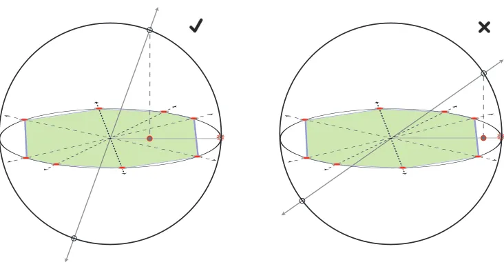
Figure 3: Geometry underlying EFS. A union of two disjoint subspaces of different dimension: the convex hull of a set of points (red circles) living on a 2D subspace is shaded (green). In (a), we show an example where EFS is guaranteed—the projection of points along the 1D subspace lie inside the shaded region. In (b), we show an example where EFS is not guaranteed—the projection of points along the 1D subspace lie outside the shaded region.

3.2.4 GEOMETRYUNDERLYINGEFSWITHOMP

The main idea underlying the proof of Theorem 1 is that, at each iteration of Algorithm 1, we require that the residual used to select a point to be included in the feature set is closer to a point in thecorrect subspace cluster(

Y

_i) than a point in anincorrect subspace cluster(

Y

_−i). To be precise, we require that the normalized inner product of the residual signals and all points outside of the correct subspace cluster

max y∈Y_−i

|hs,y_i|

ks_k2

<r(Yi), (8)

at each iteration of Algorithm 1. To provide the result in Theorem 1, we require that (8) holds for alls∈

S

_i, or all possible residual vectors.

A geometric interpretation of the EFS condition in Theorem 1 is that the orthogonal projection of all points outside of a subspace must lie within the antipodal convex hull of the set of normalized points that span the subspace. To see this, consider the projection of the points in

Y

_−i onto

S

_i. Let z∗_j denote the point on subspace

S

ithat is closest to the signalyj∈

Y

−i,

z∗_j =arg min

z∈Si kz−yjk2.

By definition, the normalized inner product of the residual with points in incorrect subspace clusters is upper bounded as

max yj∈Y−i

|hs,yji|

ks_k2 ≤ max yj∈Y−i

|hz∗_j,yji|

kz∗_jk2

= max

yj∈Y−i

cos∠{z∗_j,yj}

Thus to guarantee EFS, we require that the cosine of the angle between all signals in

Y

_−i and their projection onto

S

_iis less than the inradius of

Y

_i. Said another way, the EFS condition requires that the length of all projected points be less than the inradius of

Y

i.

In Figure 3, we provide a geometric visualization of the EFS condition for a union of disjoint subspaces (union of a 1D subspace with a 2D subspace). In (a), we show an example where EFS is guaranteed because the projection of the points outside of the 2D subspace lie well within the antipodal convex hull of the points along the normalized 2D subspace (ring). In (b), we show an example where EFS is not guaranteed because the projection of the points outside of the 2D subspace lie outside of the antipodal convex hull of the points along the normalized 2D subspace (ring).

3.3 Connections to Previous Work

In this section, we will connect our results for OMP with previous analyses of EFS with BP for disjoint (Elhamifar and Vidal, 2010, 2013) and intersecting (Soltanolkotabi and Cand`es, 2012) sub-spaces. Following this, we will contrast the geometry underlying EFS with exact recovery condi-tions used to guarantee support recovery for both OMP and BP (Tropp, 2004, 2006).

3.3.1 SUBSPACECLUSTERING WITHBP

Elhamifar and Vidal (2010) develop the following sufficient condition for EFS to occur for BP from a union of disjoint subspaces,

max j6=i cos(θ

∗

i j) < max

e

Yi∈Wi

σmin(eYi)

√

ki

, (9)

whereW_{iis the set of all full rank sub-matricesY}e_i∈Rn×ki _{of the data matrixY}

i∈Rn×diandσmin(Yei) is the minimum singular value of the sub-matrixYei. Since we assume that all of the data points have been normalized,σmin(eYi)≤1; thus, the best case result that can be obtained is that the minimum principal angle, cos(θ∗_{i j})<1/√ki. This suggests that the minimum principal angle of the union must go to zero, that is, the union must consist of orthogonal subspaces, as the subspace dimension increases.

In contrast to the condition in (9), the conditions we provide in Theorem 1 and Corollary 1 do not depend on the subspace dimension. Rather, we require that there are enough points in each subspace to achieve a sufficiently small covering; in which case, EFS can be guaranteed for subspaces of any dimension.

Soltanolkotabi and Cand`es (2012) develop the following sufficient condition for EFS to occur for BP from a union of intersecting subspaces,

µv(Yi) =max y∈Y_−ikV(i)

T_yk

where the matrixV(i)∈Rdi×n contains the dual directions (the dual vectors for each point in

Y

i embedded inRn_{) in its columns,}3_{andr(Yi)is the inradius as defined in (6). In words, (10) requires} that the maximum coherence between any point in

Y

_−iand the dual directions contained inV₍i)be

less than the inradius of the points in

Y

_i.

To link the result in (10) to our guarantee for OMP in Theorem 1, we observe that while (10) requires that µv(Yi) (coherence between a point in a subspace cluster and the dual directions of points in a different subspace cluster) be less than the inradius, Theorem 1 requires that the mutual coherence µc(Yi) (coherence between two points in different subspace clusters) be less than the inradius minus an additional term that depends on the covering radius. For an arbitrary set of points that live on a union of subspaces, the precise relationship between the two coherence parameters µc(Yi) and µv(Yi) is not straightforward; however, when the points in each subspace cluster are distributed uniformly and at random along each subspace, the dual directions will also be distributed uniformly along each subspace.4 In this case, µv(

Y

i) will be roughly equivalent to the mutual coherenceµc(Yi).

This simplification reveals the connection between the result in (10) for BP and the condition in Theorem 1 for OMP. In particular, when µv(Yi)≈µc(Yi), our result for OMP requires that the mutual coherence is smaller than the inradius minus an additional term that is linear in the covering diameter ε. For this reason, our result in Theorem 1 is more restrictive than the result provided in (10). The gap between the two bounds shrinks to zero only when the minimum principal angle

θ∗_{i j→}π/2 (orthogonal subspaces) or when the covering diameterε_→0.

In our empirical studies, we find that when BPDN is tuned to an appropriate value of the noise parameter κ, BPDN tends to produce higher rates of EFS than OMP. This suggests that the the-oretical gap between the two approaches might not be an artifact of our current analysis; rather, there might exist an intrinsic gap between the performance of each method with respect to EFS. Nonetheless, an interesting finding from our empirical study in Section 5.4, is that despite the fact that BPDN provides better rates of EFS than OMP, OMP typically provides better clustering results than BPDN. For these reasons, we maintain that OMP offers a powerful low-complexity alternative toℓ1-minimization approaches for feature selection.

3.3.2 EXACTRECOVERYCONDITIONS FORSPARSERECOVERY

To provide further intuition about EFS in endogenous sparse recovery, we will compare the geom-etry underlying the EFS condition with the geomgeom-etry of the exact recovery condition (ERC) for sparse signal recovery methods (Tropp, 2004, 2006).

To guarantee exact support recovery for a signaly∈Rn_{which has been synthesized from a linear} combination of atoms from the sub-matrixΦΛ_∈Rn×k_{, we must ensure that our approximation of} yconsists solely of atoms fromΦΛ. Let{ϕi}i∈/Λ denote the set of atoms inΦthat are not indexed

by the setΛ. Theexact recovery condition (ERC) in Theorem 2 is sufficient to guarantee that we obtain exact support recovery for both BP and OMP (Tropp, 2004).

3. See Def. 2.2 for a formal definition of the dual directions and insight into the geometry underlying their guarantees for EFS via BP (Soltanolkotabi and Cand`es, 2012).

Theorem 2 (Tropp, 2004) For any signal supported over the sub-dictionary ΦΛ, exact support

recovery is guaranteed for both OMP and BP if

ERC(Λ) =max i∈/Λ kΦΛ

†_ϕ

ik1<1.

A geometric interpretation of the ERC is that it provides a measure of how far a projected atom

ϕi outside of the set Λlies from the antipodal convex hull of the atoms in Λ. When a projected atom lies outside of the antipodal convex hull formed by the set of points in the sub-dictionaryΦΛ,

then the ERC condition is violated and support recovery is not guaranteed. For this reason, the ERC requires that the maximum coherence between the atoms inΦis sufficiently low or thatΦis incoherent.

While the ERC condition requires a global incoherenceproperty on all of the columns ofΦ, we can interpret EFS as requiring a local incoherenceproperty. In particular, the EFS condition requires that the projection of atoms in an incorrect subspace cluster

Y

_−ionto

S

_imust be incoherent with any deep holes in

Y

i along

S

i. In contrast, we require that the points within a subspace cluster exhibit local coherence in order to produce a small covering radius.

4. EFS for Bounded Unions of Subspaces

In this section, we study the connection between EFS and the higher-order principal angles (beyond the minimum angle) between pairs of intersecting subspaces.

4.1 Subspace Distances

To characterize the “distance” between pairs of subspaces in the ensemble, the principal angles between subspaces will prove useful. As we saw in the previous section, the first principal angle

θ0between subspaces

S

1 and

S

2of dimensionk1andk2 is defined as the smallest angle between a pair of unit vectors(u1,v1)drawn from

S

1×

S

2. The vector pair(u∗₁,v∗₁)that attains this minimum is referred to as the first set of principal vectors. The second principal angle θ1 is defined much like the first, except that the second set of principal vectors that define the second principal angle are required to be orthogonal to the first set of principal vectors(u∗₁,v∗₁). The remaining principal angles are defined recursively in this way. The sequence ofk=min(k1,k2)principal angles,θ0≤

θ1≤ ··· ≤θk−1, is non-decreasing and all of the principal angles lie between[0,π/2].

The definition above provides insight into what the principal angles/vectors tell us about the geometry underlying a pair of subspaces; in practice, however, the principal angles are not computed in this recursive manner. Rather, a computationally efficient way to compute the principal angles between two subspaces

S

_i and

S

_j is to first compute the singular values of the matrixG=ΦT

i Φj, whereΦi∈Rn×ki is an ONB that spans subspace

S

i. LetG=UΣVT denote the SVD ofGand let σi j∈[0,1]kdenote the singular values ofG, wherek=min(ki,kj)is the minimum dimension of the two subspaces. Themth smallest principal angleθi j(m)is related to themthlargest entry ofσi j via the following relationship, cos(θi j(m)) =σi j(m). For our subsequent discussion, we will refer to the singular values ofGas thecross-spectraof the subspace pair (

S

_i,

S

_j).

are equal to one. We define the overlap between two subspaces as the rank(G) or equivalently, q=_kσi jk0, whereq≥dim(Si∩

S

j).

4.2 Sufficient Conditions for EFS from Bounded Unions

The sufficient conditions for EFS in Theorem 1 and Corollary 1 reveal an interesting relationship between the covering radius, mutual coherence, and the minimum principal angle between pairs of subspaces in the ensemble. However, we have yet to reveal any dependence between EFS and higher-order principal angles. To make this connection more apparent, we will make additional assumptions about the distribution of points in the ensemble, namely that the data set produces a bounded union of subspacesrelative to the principal vectors supporting pairs of subspaces in the ensemble.

LetY= [YiYj]denote a collection of unit-norm data points, whereYiandYjcontain the points in subspaces

S

_iand

S

_j, respectively. LetG=ΦT

i Φj=UΣVT denote the SVD ofG, where rank(G) =q. LetUe=ΦiUq denote the set of left principal vectors ofGthat are associated with theqnonzero singular values inΣ. Similarly, letVe=ΦjVq denote the set of right principal vectors ofGthat are associated with the nonzero singular values inΣ. When the points in each subspace are incoherent with the principal vectors in the columns ofUe andVe, we say that the ensembleY is anbounded union of subspaces. Formally, we require the following incoherence property holds:

kY_iTUe_k∞,kYjTVek∞

≤γ, (11)

where_k·k∞is the entry-wise maximum andγ∈(0,1]. This property requires that the inner products

between the points in a subspace and the set of principal vectors that span non-orthogonal directions between a pair of subspaces is bounded by a fixed constant.

When the points in each subspace are distributed such that (11) holds, we can rewrite the mutual coherence between any two points from different subspaces to reveal its dependence on higher-order principal angles. In particular, we show (in Section 7.2) that the coherence between the residuals used in Algorithm 1 to select the next point to be included in the representation of a pointy_∈

Y

_i, and a point in

Y

_jis upper bounded by

max y∈Yj

|hs,y_i|

ks_k2 ≤

γ_kσi jk1, (12)

where γis the bounding constant of the dataY and_kσi jk1 is the ℓ1-norm of the cross-spectra or equivalently, the trace norm of G. Using the bound in (12), we arrive at the following sufficient condition for EFS from bounded unions of subspaces. We provide the proof in Section 7.2.

Theorem 3 Let Y live on a bounded union of subspaces, where q=rank(G)andγ<p1/q. Let

σi j denote the cross-spectra of the subspaces

S

i and

S

j and let εdenote the covering diameter of

Y

_i. A sufficient condition for Algorithm 1 to return exact feature sets for all points in

Y

_i is that the covering diameter

ε < min j6=i

q

1₋γ2_kσ i jk2₁.

ensemble has a small bounding constant is to constrain the total amount of energy that points in

Y

_j

have in theq-dimensional subspace spanned by the principal vectors inVe.

Our analysis for bounded unions assumes that the nonzero entries of the cross-spectra are equal, and thus each pair of supporting principal vectors inVeare equally important in determining whether points in

Y

iwill admit EFS. However, this assumption is not true in general. When the union is sup-ported by principal vectors with non-uniform principal angles, our analysis suggests that a weaker form of incoherence is required. Instead of requiring incoherence with all principal vectors, the data must be sufficiently incoherent with the principal vectors that correspond to small principal angles (or large values of the cross-spectra). This means that as long as points are not concentrated along the principal directions with small principal angles (i.e., intersections), then EFS can be guaranteed, even when subspaces exhibit non-trivial intersections. To test this prediction, we will study EFS for abounded energy modelin Section 5.2. We show that when the data set is sparsely sampled (larger covering radius), reducing the amount of energy that points contain in subspace intersections, does in fact increase the probability that points admit EFS.

Finally, our analysis of bounded unions suggests that the decay of the cross-spectra is likely to play an important role in determining whether points will admit EFS or not. To test this hypothesis, we will study the role that the structure of the cross-spectra plays in EFS in Section 5.3.

5. Experimental Results

In our theoretical analysis of EFS in Sections 3 and 4, we revealed an intimate connection between the covering radius of subspaces and the principal angles between pairs of subspaces in the en-semble. In this section, we will conduct an empirical study to explore these connections further. In particular, we will study the probability of EFS as we vary the covering radius as well as the dimension of the intersection and/or overlap between subspaces.

5.1 Generative Model for Synthetic Data

In order to study EFS for unions of subspaces with varied cross-spectra, we will generate synthetic data from unions of overlappingblock sparse signals.

5.1.1 CONSTRUCTINGSUB-DICTIONARIES

We construct a pair of sub-dictionaries as follows: Take two subsetsΩ1andΩ2ofksignals (atoms) from a dictionaryDcontainingMatoms_{dm}Mm=1in its columns, wheredm∈Rnand|Ω1|=|Ω2|= k. LetΨ_∈Rn×k _{denote the subset of atoms indexed by} Ω1,and let Φ_∈Rn×k _{denote the subset} of atoms indexed byΩ2. Our goal is to selectΨ andΦ such thatG=ΨT_{Φ is diagonal, that is,}

hψi,φji=0,ifi6=j, whereψiis theithelement inΨandφjis the jthelement ofΦ. In this case, the cross-spectra is defined asσ=diag(G), whereσ_∈[0,1]k_{. For each union, we fix the “overlap”qor} the rank ofG=ΨT_{Φto a constant between zero (orthogonal subspaces) andk(maximal overlap).}

To generate a pair of k-dimensional subspaces with a q-dimensional overlap, we can pair the elements fromΨandΦsuch that theithentry of the cross-spectra equals

σ(i) = (

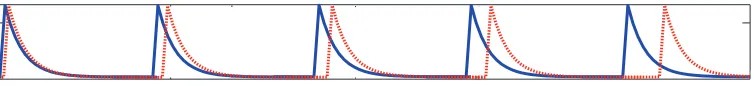
Figure 4: Generating unions of subspaces from shift-invariant dictionaries. An example of a col-lection of two sub-dictionaries of five atoms, where each of the atoms have a non-zero inner product with one other atom. This choice of sub-dictionaries produces a union of disjoint subspaces, where the overlap ratioδ=q/k=1.

We can leverage the banded structure of shift-invariant dictionaries, for example, dictionary matrices with localized Toeplitz structure, to generate subspaces with structured cross-spectra as follows.5 First, we fix a set ofkincoherent (orthogonal) atoms from our shift-invariant dictionary, which we place in the columns ofΨ. Now, holdingΨfixed, we set the ith atomφi of the second sub-dictionaryΦto be a shifted version of theithatomψiof the dictionaryΨ. To be precise, if we setψi=dm, wheredmis themth atom in our shift-invariant dictionary, then we will setφi=dm+∆

for a particular shift∆. By varying the shift∆, we can control the coherence betweenψi andϕi. In Figure 4, we show an example of one such construction fork=q=5. Sinceσ_∈(0,1]k_{, the} worst-case pair of subspaces with overlap equal to q is obtained when we pair q identical atoms with k₋qorthogonal atoms. In this case, the cross-spectra attains its maximum over its entire support and equals zero otherwise. For such unions, the overlapqequals the dimension of the intersection between the subspaces. We will refer to this class of block-sparse signals as orthoblock sparse signals.

5.1.2 COEFFICIENTSYNTHESIS

To synthesize a point that lives in the span of the sub-dictionaryΨ_∈Rn×k_{, we combine the elements}

{ψ1, . . . ,ψk}and subspace coefficients{α(1), . . . ,α(k)}linearly to form

yi= k

∑

j=1

ψjα(j),

whereα(j) is the subspace coefficient associated with the jth column inΨ. Without loss of gen-erality, we will assume that the elements inΨare sorted such that the values of the cross-spectra are monotonically decreasing. Letyc_i =∑q_j=1ψjαi(j)be the “common component” ofyi that lies in the space spanned by the principal directions between the pair of subspaces that correspond to non-orthogonal principal angles between(Φ,Ψ) and let yd_i =∑kj=q+1ψjα(j) denote the “disjoint component” of yi that lies in the space orthogonal to the space spanned by the first q principal directions.

For our experiments, we consider points drawn from one of the two following coefficient distri-butions, which we will refer to as(M1)and(M2)respectively.

• (M1) Uniformly Distributed on the Sphere: Generate subspace coefficients according to a standard normal distribution and map the point to the unit sphere

yi=

∑jψjα(j)

k∑jψjα(j)k2

, whereα(j)_∼

N

(0,1).

• (M2) Bounded Energy Model:Generate subspace coefficients according to(M1)and rescale each coefficient in order to bound the energy in the common component

yi= τyc_i

kyc ik2

+(1−τ)y

d i

kyd ik2

.

By simply restricting the total energy that each point has in its common component, the bounded energy model (M2) can be used to produce ensembles with small bounding constant to test the predictions in Theorem 3.

5.2 Phase Transitions for OMP

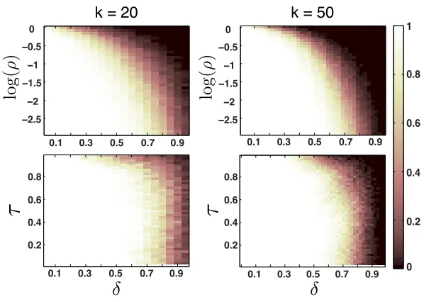
The goal of our first experiment is to study the probability of EFS—the probability that a point in the ensemble admits exact features—as we vary both the number and distribution of points in each subspace as well as the dimension of the intersection between subspaces. For this set of experiments, we generate a union of orthoblock sparse signals, where the overlap equals the dimension of the intersection.

Along the top row of Figure 5, we display the probability of EFS for orthoblock sparse signals generated according to the coefficient model(M1): the probability of EFS is computed as we vary theoverlap ratioδ=q/k∈[0,1]in conjunction with theoversampling ratioρ=k/d∈[0,1], where q=rank(ΦT

1Φ2)equals the dimension of the intersection between the subspaces, anddis the num-ber of points per subspace. Along the bottom row of Figure 5, we display the probability of EFS for orthoblock sparse signals generated according to the coefficient model (M2): the probability of EFS is computed as we vary the overlap ratioδand the amount of energy τ_∈[0,1)each point has within its common component. For these experiments, the subspace dimension is set tok=20 (left) andk=50 (right). To see the phase boundary that arises when we approach critical sampling (i.e.,ρ_≈1), we display our results in terms of the logarithm of the oversampling ratio. For these experiments, the results are averaged over 500 trials.

k =50

0.1 0.3 0.5 0.7 0.9 −2.5

−2 −1.5

−1 −0.5

0

0 0.2 0.4 0.6 0.8 1

−2.5 −2 −1.5

−1 −0.5

0

0.1 0.3 0.5 0.7 0.9

0.2 0.4 0.6 0.8

0.1 0.3 0.5 0.7 0.9

k = 50, m= 1000

0.2 0.4 0.6 0.8

0.1 0.3 0.5 0.7 0.9

k = 20 k = 50

Figure 5: Probability of EFS for different coefficient distributions. The probability of EFS for a union of two subspaces of dimensionk=20 (left column) andk=50 (right column). The probability of EFS is displayed as a function of the overlap ratioδ_∈[0,1)and the logarithm of the oversampling ratio log(ρ) (top row) and the mutual energy τ=_kyck2 (bottom row) .

Along the bottom row of Figure 5, we study the impact of the bounding constant on EFS, as discussed in Section 4.2. In this experiment, we fix the oversampling ratio toρ=0.1 and vary the common energyτ in conjunction with the overlap ratioδ. By reducing the bounding constant of the union, the phase boundary for the uniformly distributed data from model(M1)is shifted from

δ=0.45 toδ=0.7 for bothk=20 andk=50. This result confirms our predictions in the discussion of Theorem 3 that by reducing the amount of energy that points have in their subspace intersections EFS will occur for higher degrees of overlap. Another interesting finding of this experiment is that, onceτreaches a threshold, the phase boundary remains constant and further reducing the bounding constant has no impact on the phase transitions for EFS.

5.3 Comparison of OMP and NN

In this section, we compare the probability of EFS for feature selection with OMP and nearest neighbors (NN). First, we compare the performance of both feature selection methods for unions with different cross-spectra. Second, we compare the phase transitions for unions of orthoblock sparse signals as we vary the overlap and oversampling ratio.

Overlap Ratio ( ) Overlap Ratio ( )

.9 .95 1

0.25 0.5 0.75 1 Probability of EFS

0.25 0.5 0.75 1 .2

.6 1

Probability of EFS

0.25 0.5 0.75 1 0

0.5 1

Probability of EFS

Overlap Ratio ( ) 0 5 10 15 20 0

0.5 1

( = 0.75)

Singular value index

5 10 15 20 0

0.5 1

( = 1)

Singular value index

0 _{5 10 15 20} 0.5

1

( = 1)

Singular value index

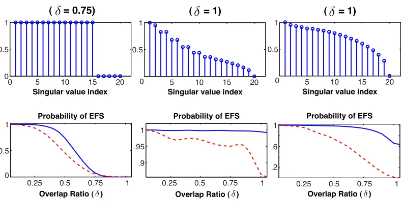
Figure 6: Probability of EFS for unions with structured cross-spectra. Along the top row, we show the cross-spectra for different unions of block-sparse signals. Along the bottom row, we show the probability of EFS as we vary the overlap ratioδ_∈[0,1]for OMP (solid) and NN (dash).

columns, respectively. Along the bottom row of Figure 6, we show the probability of EFS for OMP and NN for each of these three subspace unions as we vary the overlapq. To do this, we generate subspaces by setting their cross-spectra equal to the first q entries equal to the cross-spectra in Figure 6 and setting the remainingk₋qentries of the cross-spectra equal to zero. Each subspace cluster is generated by samplingd=100 points from each subspace according to the coefficient model(M1).

0.2

0.3

0.4

0.5

0.6

0.7

0.8

0.9

0.2 0.4 0.6 0.8 1 0

0.2 0.4 0.6 0.8 1

0.2

0.3

0.4

0.5

0.6

0.7

0.8

0.9

0.2 0.4 0.6 0.8 1

(a) (b)

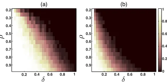
Figure 7: Phase transitions for OMP and NN. The probability of EFS for orthoblock sparse signals for OMP (a) and NN (b) feature sets as a function of the oversampling ratioρ=k/dand the overlap ratioδ=q/k, wherek=20.

In Figure 7, we display the probability of EFS for OMP (left) and sets of NN (right) as we vary the overlap and the oversampling ratio. For this experiment, we consider unions of orthoblock sparse signals living on subspaces of dimensionk=50 and varyρ_∈[0.2,0.96]andδ_∈[1/k,1]. An interesting result of this study is that there are regimes where the probability of EFS equals zero for NN but occurs for OMP with a non-trivial probability. In particular, we observe that when the sampling of each subspace is sparse (the oversampling ratio is low), the gap between OMP and NN increases and OMP significantly outperforms NN in terms of their probability of EFS. Our study of EFS for structured cross-spectra suggests that the gap between NN and OMP should be even more pronounced for cross-spectra with superlinear decay.

5.4 Clustering Illumination Subspaces

In this section, we compare the performance of sparse recovery methods, that is, BP and OMP, with NN for clustering unions of illumination subspacesarising from a collection of images of faces under different lighting conditions. By fixing the camera center and position of the persons face and capturing multiple images under different lighting conditions, the resulting images can be well-approximated by a 5-dimensional subspace (Ramamoorthi, 2002).

In Figure 2, we show three examples of the subspace affinity matrices obtained with NN, BP, and OMP for two different faces under 64 different illumination conditions from the Yale Database B (Georghiades et al., 2001), where each image has been subsampled to 48_×42 pixels, withn=2016. In all of the examples, the data is sorted such that the images for each face are placed in a contiguous block.

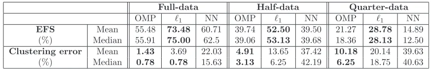
Table 1: Classification and EFS rates for illumination subspaces. Shown are the aggregate results obtained over 38₂pairs of subspaces.

k≤5 coefficients.6 _{The resulting coefficient vectors are then stacked into the rows of a matrixCand} the final subspace affinityWis computed by symmetrizing the coefficient matrix,W =_|C_|+_|CT_|.

After computing the subspace affinity matrix for each of these three feature selection methods, we employ a spectral clustering approach which partitions the data based upon the eigenvector corresponding to the smallest nonzero eigenvalue of the graph Laplacian of the affinity matrix (Shi and Malik, 2000; Ng et al., 2002). For all three feature selection methods, we obtain the best clustering performance when we cluster the data based upon the graph Laplacian instead of the normalized graph Laplacian (Shi and Malik, 2000). In Table 1, we display the percentage of points that resulted in EFS and the classification error for all pairs of 38₂subspaces in the Yale B database. Along the top row, we display the mean and median percentage of points that resulted in EFS for the full data set (all 64 illumination conditions), half of the data set (32 illumination conditions selected at random in each trial), and a quarter of the data set (16 illumination conditions selected at random in each trial). Along the bottom row, we display the clustering error (percentage of points that were incorrectly classified) for SSC-OMP, SSC, and NN-based clustering (spectral clustering of the NN affinity matrix).

While both sparse recovery methods (BPDN and OMP) admit EFS rates that are comparable to NN on the full data set, we find that sparse recovery methods provide higher rates of EFS than NN when the sampling of each subspace is sparse, that is, the half and quarter data sets. These results are also in agreement with our experiments on synthetic data. A surprising result is that SSC-OMP provides better clustering performance than SSC on this particular data set, even though BP provides higher rates of EFS.

6. Discussion

In this section, we provide insight into the implications of our results for different applications of sparse recovery and compressive sensing. Following this, we end with some open questions and directions for future research.

6.1 “Data Driven” Sparse Approximation

The standard paradigm in signal processing and approximation theory is to compute a representation of a signal in a fixed and pre-specified basis or overcomplete dictionary. In most cases, the

naries used to form these representations are designed according to some mathematical desiderata. A more recent approach has been to learn a dictionary from a collection of data, such that the data admit a sparse representation with respect to the learned dictionary (Olshausen and Field, 1997; Aharon et al., 2006).

The applicability and utility of endogenous sparse recovery in subspace learning draws into question whether we can use endogenous sparse recovery for other tasks, including approximation and compression. The question that naturally arises is, “do we design a dictionary, learn a dictionary, or use the data as a dictionary?” Understanding the advantages and tradeoffs between each of these approaches is an interesting and open question.

6.2 Learning Block-Sparse Signal Models

Block-sparse signals and other structured sparse signals have received a great deal of attention over the past few years, especially in the context of compressive sensing from structured unions of subspaces (Lu and Do, 2008; Blumensath and Davies, 2009) and in model-based compressive sensing (Baraniuk et al., 2010). In all of these settings, the fact that a class or collection of signals admit structured support patterns is leveraged in order to obtain improved recovery of sparse signals in noise and in the presence of undersampling.

To exploit such structure in sparse signals—especially in situations where the structure of sig-nals or blocks of active atoms may be changing across different instances in time, space, etc.—the underlying subspaces that the signals occupy must be learned directly from the data. The meth-ods that we have described for learning union of subspaces from ensembles of data can be used in the context of learning block sparse and other structured sparse signal models. The application of subspace clustering methods for this purpose is an interesting direction for future research.

6.3 Beyond Coherence

While the maximum and cumulative coherence provide measures of the uniqueness of sub-dictionaries that are necessary to guarantee exact signal recovery for sparse recovery methods (Tropp, 2004) , our current study suggests that examining the principal angles formed from pairs of sub-dictionaries could provide an even richer description of the geometric properties of a dictionary. Thus, a study of the principal angles formed by different subsets of atoms from a dictionary might provide new insights into the performance of sparse recovery methods with coherent dictionaries and for com-pressive sensing from structured matrices. In addition, our empirical results in Section 5.3 suggest that there might exist an intrinsic difference between sparse recovery from dictionaries that exhibit sublinear versus superlinear decay in their principal angles or cross-spectra. It would be interesting to explore whether these two “classes” of dictionaries exhibit different phase transitions for sparse recovery.

6.4 Discriminative Dictionary Learning

admit a more compact representation with respect to the dictionary that was learned from the class of signals that the test signal belongs to.

Instead of learning these dictionaries independently of one another, discriminative dictionary learning (Mairal et al., 2008; Ramirez et al., 2010), aims to learn a collection of dictionaries

{Φ1,Φ2, . . . ,Φp} that are incoherent from one another. This is accomplished by minimizing ei-ther the spectral (Mairal et al., 2008) or Frobenius norm (Ramirez et al., 2010) of the matrix product

ΦT

i Φjbetween pairs of dictionaries. This same approach may also be used to learn sensing matrices for CS that are incoherent with a learned dictionary (Mailh`e et al., 2012).

There are a number of interesting connections between discriminative dictionary learning and our current study of EFS from collections of unions of subspaces. In particular, our study provides new insights into the role that the principal angles between two dictionaries tell us about our ability to separate classes of data based upon their sparse representations. Our study of EFS from unions with structured cross-spectra suggests that the decay of the cross-spectra between different data classes provides a powerful predictor of the performance of sparse recovery methods from data living on a union of low-dimensional subspaces. This suggests that in the context of discriminative dictionary learning, it might be more advantageous to reduce theℓ1-norm of the cross-spectra rather than simply minimizing the maximum coherence and/or Frobenius norm between points in different subspaces. To do this, each class of data must first be embedded within a subspace, a ONB is formed for each subspace, and then theℓ1- norm of the cross-spectra must be minimized. An interesting question is how one might impose such a constraint in discriminative dictionary learning methods.

6.5 Open Questions and Future Work

While EFS provides a natural measure of how well a feature selection algorithm will perform for the task of subspace clustering, our empirical results suggest that EFS does not necessarily predict the performance of spectral clustering methods when applied to the resulting subspace affinity matrices. In particular, we find that while OMP obtains lower rates of EFS than BPDN on real-world data, OMP yields better clustering results on the same data set. Understanding where this difference in performance might arise from is an interesting direction for future research.

Another interesting finding of our empirical study is that the gap between the rates of EFS for sparse recovery methods and NN depends on the sampling density of each subspace. In particular, we found that for dense samplings of each subspace, the performance of NN is comparable to sparse recovery methods; however, when each subspace is more sparsely sampled, sparse recovery methods provide significant gains over NN methods. This result suggests that endogenous sparse recovery provides a powerful strategy for clustering when the sampling of subspace clusters is sparse. Analyzing the gap between sparse recovery methods and NN methods for feature selection is an interesting direction for future research.

7. Proofs

In this section, we provide proofs for main theorems in the paper.

7.1 Proof of Theorem 1

Consider the greedy selection step in OMP (see Algorithm 1) for a pointyiwhich belongs to the subspace cluster

Y

k. Recall that at themthstep of OMP, the point that is maximally correlated with the signal residual will be selected to be included in the feature setΛ. The normalized residual at themthstep is computed as

sm= (I−PΛ)yi k(I₋PΛ)yik2

,

where PΛ =YΛYΛ† ∈Rn×n is a projector onto the subspace spanned by the points in the current

feature setΛ, where_|Λ_|=m₋1.

To guarantee that we select a point from

S

_k, we require that the following greedy selection criterion holds:

max v∈Yk

|hsm,v_i|>max v∈/Yk

|hsm,v_i|.

We will prove that this selection criterion holds at each step of OMP by developing an upper bound on the RHS (the maximum inner product between the residual and a point outside of

Y

_k) and a lower bound on the LHS (the minimum inner product between the residual and a point in

Y

k).

First, we will develop the upper bound on the RHS. In the first iteration, the residual is set to the signal of interest (yi). In this case, we can bound the RHS by the mutual coherence µc= maxi6=jµc(Yi,

Y

j)across all other sets

max yj∈/Yk

|hyi,yji| ≤µc.

Now assume that at themthiteration we have selected points from the correct subspace cluster. This implies that our signal residual still lies within the span of

Y

_k, and thus we can write the residual sm=z+e, wherezis the closest point to sm in

Y

k andeis the remaining portion of the residual which also lies in

S

_k. Thus, we can bound the RHS as follows

max yj∈/Yk

|hsm,yji|=max yj∈/Yk

|hz+e,yji|

≤max

yj∈/Yk

|hz,yji|+|he,yji|

≤µc+max yj∈/Yk

|he,yji|

≤µc+cos(θ0)kek2kyik2,

whereθ0is the minimum principal angle between

S

kand all other subspaces in the ensemble. Using the fact that cover(Yk) =ε/2, we can bound theℓ2-norm of the vectoreas

ke_k2=ks−zk2

= q

ks_k2₂+_kz_k2₂₋2_|hs,z_i|

≤ r

2₋2

q

1₋(ε/2)2

= q

2₋p4₋ε2_.

Plugging this quantity into our expression for the RHS, we arrive at the following upper bound

max yj∈/Yk

|hsm,yji| ≤µc+cos(θ0)

q

2₋p4₋ε2_<µ

c+cos(θ0)

ε 4 √

where the final simplification comes from invoking the following Lemma.

Lemma 1 For 0_≤x_≤1, _q

2₋p4₋x2_≤ x

4 √

12.

Proof of Lemma 1:We wish to develop an upper bound on the function

f(x) =2₋p4₋x2_{, for 0≤x≤1.}

Thus our goal is to identify a functiong(x), where f′(x)_≤g′(x) for 0_≤x_≤1, andg(0) = f(0). The derivative of f(x)can be upper bounded easily as follows

f′(x) =√ x

4₋x2 ≤ x

√

3, for 0≤x≤1.

Thus,g′(x) =x/√3,andg(x) =x2/√12; this ensures that f′(x)_≤g′(x)for 0_≤x_≤1, andg(0) =

f(0). By the Fundamental Theorem of Integral Calculus, g(x)provides an upper bound for f(x)

over the domain of interest where, 0_≤x_≤1.To obtain the final result, take the square root of both

sides,p2₋√4₋x2_≤

q

x2_/√_12=x/√4

12.

Second, we will develop the lower bound on the LHS of the greedy selection criterion. To ensure that we select a point from

Y

_k at the first iteration, we require thatyi’s nearest neighbor belongs to the same subspace cluster. Letyi_nndenote the nearest neighbor toyi

yi_nn=arg max

j6=i |hyi,yji|.

Ifyi_nnandyiboth lie in

Y

k, then the first point selected via OMP will result in EFS.

Let us assume that the points in

Y

_k admit an ε-covering of the subspace cluster

S

_k, or that cover(Yk) =ε/2. In this case, we have the following bound in effect

max yj∈Yk

|hsm,yji| ≥

r

1₋ε 2 4.

Putting our upper and lower bound together and rearranging terms, we arrive at our final condi-tion on the mutual coherence

µc<

r

1₋ε 2

4 −cos(θ0)

ε 4 √

12.

Since we have shown that this condition is sufficient to guarantee EFS at each step of Algorithm 1 provided the residual stays in the correct subspace, Theorem 1 follows by induction.

7.2 Proof of Theorem 3