Kernel Bayes' Rule: Bayesian Inference with Positive Definite Kernels

Kernel Bayes’ Rule: Bayesian Inference with Positive Definite Kernels

Kenji Fukumizu [email protected]

The Institute of Statistical Mathematics 10-3 Midoricho, Tachikawa

Tokyo 190-8562 Japan

Le Song [email protected]

College of Computing

Georgia Institute of Technology 1340 Klaus Building, 266 Ferst Drive Atlanta, GA 30332, USA

Arthur Gretton [email protected]

Gatsby Computational Neuroscience Unit University College London

Alexandra House, 17 Queen Square London, WC1N 3AR, UK

Editor:Ingo Steinwart

Abstract

A kernel method for realizing Bayes’ rule is proposed, based on representations of probabilities in reproducing kernel Hilbert spaces. Probabilities are uniquely characterized by the mean of the canonical map to the RKHS. The prior and conditional probabilities are expressed in terms of RKHS functions of an empirical sample: no explicit parametric model is needed for these quan-tities. The posterior is likewise an RKHS mean of a weighted sample. The estimator for the expectation of a function of the posterior is derived, and rates of consistency are shown. Some rep-resentative applications of the kernel Bayes’ rule are presented, including Bayesian computation without likelihood and filtering with a nonparametric state-space model.

Keywords: kernel method, Bayes’ rule, reproducing kernel Hilbert space

1. Introduction

Kernel methods have long provided powerful tools for generalizing linear statistical approaches to nonlinear settings, through an embedding of the sample to a high dimensional feature space, namely a reproducing kernel Hilbert space (RKHS) (Sch¨olkopf and Smola, 2002). Examples include sup-port vector machines, kernel PCA, and kernel CCA, among others. In these cases, data are mapped via a canonical feature map to a reproducing kernel Hilbert space (of high or even infinite dimen-sion), in which the linear operations that define the algorithms are implemented. The inner product between feature mappings need never be computed explicitly, but is given by a positive definite kernel function unique to the RKHS: this permits efficient computation without the need to deal explicitly with the feature representation.

kernel meansof the underlying random variables. With an appropriate choice of positive definite kernel, the kernel mean on the RKHS uniquely determines the distribution of the variable (Fukumizu et al., 2004, 2009a; Sriperumbudur et al., 2010), and statistical inference problems on distributions can be solved via operations on the kernel means. Applications of this approach include homo-geneity testing (Gretton et al., 2007; Harchaoui et al., 2008; Gretton et al., 2009a, 2012), where the empirical means on the RKHS are compared directly, and independence testing (Gretton et al., 2008, 2009b), where the mean of the joint distribution on the feature space is compared with that of the product of the marginals. Representations of conditional dependence may also be defined in RKHS, and have been used in conditional independence tests (Fukumizu et al., 2008; Zhang et al., 2011).

In this paper, we propose a novel, nonparametric approach to Bayesian inference, making use of kernel means of probabilities. In applying Bayes’ rule, we compute the posterior probability ofx in

X

given observationyin

Y

;

q(x_|y) = p(y|x)π(x)

qY(y)

, (1)

where π(x) and p(y_|x) are the density functions of the prior and the likelihood of y givenx, re-spectively, with respective base measuresνX andνY, and the normalization factorqY(y) is given

by

qY(y) =

Z

p(y_|x)π(x)dνX(x).

Our main result is a nonparametric estimate of posterior kernel mean, given kernel mean represen-tations of the prior and likelihood. We call this methodkernel Bayes’ rule.

A valuable property of the kernel Bayes’ rule is that the kernel posterior mean is estimated nonparametrically from data. The prior is represented by a weighted sum over a sample, and the probabilistic relation expressed by the likelihood is represented in terms of a sample from a joint distribution having the desired conditional probability. This confers an important benefit: we can still perform Bayesian inference by making sufficient observations on the system, even in the ab-sence of a specific parametric model of the relation between variables. More generally, if we can sample from the model, we do not require explicit density functions for inference. Such situations are typically seen when the prior or likelihood is given by a random process: Approximate Bayesian Computation (Tavar´e et al., 1997; Marjoram et al., 2003; Sisson et al., 2007) is widely applied in population genetics, where the likelihood is expressed as a branching process, and nonparametric Bayesian inference (M¨uller and Quintana, 2004) often uses a process prior with sampling methods. Alternatively, a parametric model may be known, however it might be of sufficient complexity to require Markov chain Monte Carlo or sequential Monte Carlo for inference. The present kernel approach provides an alternative strategy for Bayesian inference in these settings. We demonstrate consistency for our posterior kernel mean estimate, and derive convergence rates for the expectation of functions computed using this estimate.

Kankainen and Ushakov, 1998) to representing probabilities. A well conditioned empirical estimate of the characteristic function can be difficult to obtain, especially for conditional probabilities. By contrast, the kernel mean has a straightforward empirical estimate, and conditioning and marginal-ization can be implemented easily, at a reasonable computational cost.

The proposed method of realizing Bayes’ rule is an extension of the approach used by Song et al. (2009) for state-space models. In this earlier work, a heuristic approximation was used, where the kernel mean of the new hidden state was estimated by adding kernel mean estimates from the previous hidden state and the observation. Another relevant work is the belief propagation approach in Song et al. (2010a, 2011), which covers the simpler case of a uniform prior.

This paper is organized as follows. We begin in Section 2 with a review of RKHS terminology and of kernel mean embeddings. In Section 3, we derive an expression for Bayes’ rule in terms of kernel means, and provide consistency guarantees. We apply the kernel Bayes’ rule in Section 4 to various inference problems, with numerical results and comparisons with existing methods in Section 5. Our proofs are contained in Section 6 (including proofs of the consistency results of Section 3).

2. Preliminaries: Positive Definite Kernels and Probabilities

Throughout this paper, all Hilbert spaces are assumed to be separable. For an operatorAon a Hilbert space, the range is denoted by

R

(A). The linear hull of a subsetSin a vector space is denoted by SpanS.

We begin with a review of positive definite kernels, and of statistics on the associated reproduc-ing kernel Hilbert spaces (Aronszajn, 1950; Berlinet and Thomas-Agnan, 2004; Fukumizu et al.,

2004, 2009a). Given a set Ω, a (R_{-valued) positive definite kernel k on} Ωis a symmetric kernel

k:Ω_×Ω_→R_{such that∑}n_{i,j=1cicjk(xi,xj)≥0 for arbitrary number of pointsx1, . . . ,xninΩand} real numbers c1, . . . ,cn. The matrix (k(xi,xj))ni,j=1 is called a Gram matrix. It is known by the

Moore-Aronszajn theorem (Aronszajn, 1950) that a positive definite kernel onΩuniquely defines a

Hilbert space

H

consisting of functions onΩsuch that the following three conditions hold:

(i) k(_·,x)_∈

H

for anyx_∈Ω,

(ii) Span_{k(_·,x)_|x_∈Ω_}is dense in

H

,

(iii) _hf,k(_·,x)_i= f(x) for anyx_∈Ωand f _∈

H

(the reproducing property), where _h·,_·iis the inner product of

H

.

The Hilbert space

H

is called thereproducing kernel Hilbert space(RKHS) associated withk, since

the functionkx=k(·,x)serves as the reproducing kernelhf,kxi= f(x)for f∈

H

.

A positive definite kernel onΩis said to beboundedif there isM>0 such thatk(x,x)_≤Mfor anyx_∈Ω.

Let(

X

,

B

X)be a measurable space,Xbe a random variable taking values in

X

with distribution

PX, andkbe a measurable positive definite kernel on

X

such thatE[pk(X,X)]<∞. The associated

RKHS is denoted by

H

. Thekernel mean mk_X (also writtenmk_PX) ofXon the RKHS

H

is defined by the mean of the

H

-valued random variablek(_·,X). The existence of the kernel mean is guaranteed by E[_kk(_·,X)_k] =E[pk(X,X)]<∞. We will generally write mX in place of mk_X for simplicity, where there is no ambiguity. By the reproducing property, the kernel mean satisfies the relation

for any f ∈

H

. Plugging f =k(_·,u)into this relation,

mX(u) =E[k(u,X)] = Z

k(u,x˜)dPX(x˜), (3)

which shows the explicit functional form. The kernel meanmX is also denoted bymPX, as it depends

only on the distributionPX withkfixed.

Let (

X

,

B

X) and(

Y

,

B

Y) be measurable spaces, (X,Y) be a random variable on

X

×

Y

with

distribution P, andkX andkY be measurable positive definite kernels with respective RKHS

H

X

and

H

_Y such thatE[kX(X,X)]<∞andE[kY(Y,Y)]<∞. The (uncentered)covariance operator

CY X :

H

X →

H

Y is defined as the linear operator that satisfies

hg,CY Xf_iHY =E[f(X)g(Y)]

for all f_∈

H

X,g∈

H

Y. This operatorCY X can be identified withm(Y X)in the product space

H

Y⊗

H

X, which is given by the product kernel kYkX on

Y

×

X

(Aronszajn, 1950), by the standard

identification between the linear maps and the tensor product. We also defineCX X for the operator on

H

X that satisfieshf2,CX Xf1i=E[f2(X)f1(X)]for any f1,f2∈

H

X. Similarly to Equation (3),

the explicit integral expressions forCY X andCX X are given by

(CY Xf)(y) = Z

kY(y,y˜)f(x˜)dP(x˜,y˜) and (CX Xf)(x) = Z

kX(x,x˜)f(x˜)dPX(x˜), (4)

respectively.

An important notion in statistical inference with positive definite kernels is the characteristic property. A bounded measurable positive definite kernelk on a measurable space(Ω,

B

)is called characteristic if the mapping from a probability Qon (Ω,

B

) to the kernel mean mk_Q∈

H

is in-jective (Fukumizu et al., 2009a; Sriperumbudur et al., 2010). This is equivalent to assuming that EX∼P[k(·,X)] =EX′_∼Q[k(·,X′)]impliesP=Q: probabilities are uniquely determined by their kernel

means on the associated RKHS. With this property, problems of statistical inference can be cast as inference on the kernel means. A popular example of a characteristic kernel defined on Euclidean space is the Gaussian RBF kernelk(x,y) =exp(_−kx₋y_k2/(2σ2_{)). A bounded measurable positive}

definite kernel on a measurable space(Ω,

B

)with corresponding RKHS

H

is characteristic if and

only if

H

+R_{is dense in L}2_{(P) for arbitrary probabilityPon (Ω,}

B

), where

H

+R_{is the direct}

sum of two RKHSs

H

andR_{(Aronszajn, 1950). This implies that the RKHS defined by a}

char-acteristic kernel is rich enough to be dense inL2 space up to the constant functions. Other useful conditions for a kernel to be characteristic can be found in Sriperumbudur et al. (2010), Fukumizu et al. (2009b), and Sriperumbudur et al. (2011).

Throughout this paper, when positive definite kernels on a measurable space are discussed, the following assumption is made:

(K) Positive definite kernels are bounded and measurable.

Under this assumption, the mean and covariance always exist for arbitrary probabilities.

Given i.i.d. sample(X1,Y1), . . . ,(Xn,Yn)with lawP, the empirical estimators of the kernel mean and covariance operator are given straightforwardly by

b

m(_Xn)= 1

n n

∑

i=1

kX(·,Xi), Cb_{Y X}(n)=1

n n

∑

i=1

whereCb_{Y X}(n) is written in tensor form. These estimators are √n-consistent in appropriate norms, and√n(m_bX(n)₋mX) converges to a Gaussian process on

H

X (Berlinet and Thomas-Agnan, 2004,

Section 9.1). While we may use non-i.i.d. samples for numerical examples in Section 5, in our theoretical analysis we always assume i.i.d. samples for simplicity.

3. Kernel Expression of Bayes’ Rule

We review Bayes’ rule and the notion of kernel conditional mean embeddings in Section 3.1. We demonstrate that Bayes’ rule may be expressed in terms of these conditional mean embeddings. We provide consistency results for the empirical estimators of the conditional mean embedding for the posterior in Section 3.2.

3.1 Kernel Bayes’ Rule

We first review Bayes’ rule in a general form without using density functions, since the kernel Bayes’ rule can be applied to situations where density functions are not available.

Let(

X

,

B

X)and(

Y

,

B

Y)be measurable spaces,(Ω,

A

,P)a probability space, and(X,Y):Ω→

X

_×

Y

be a (X _×

Y

-valued) random variable with distributionP. The marginal distribution ofX

is denoted by PX. Suppose that Πis a probability measure on (

X

,

B

X), which serves as aprior

distribution. For eachx_∈

X

, letPY_|x denote the conditional probability ofY givenX =x; namely, PY_|x(B) =E[IB(Y)|X =x], where IB is the indicator function of a measurable set B∈

B

Y.1 We

assume that the conditional probabilityPY_|x isregular; namely, it defines a probability measure on

Y

for eachx. The priorΠand the family_{PY_|x|x∈

X

}defines the joint distributionQon

X

×

Y

by

Q(A_×B) =

Z

A

PY_|x(B)dΠ(x) (5)

for anyA_∈

B

X andB∈

B

Y, and its marginal distributionQY by

QY(B) =Q(

X

×B).

Let(Z,W)be a random variable on

X

_×

Y

with distributionQ. Fory_∈

Y

, theposteriorprobability givenyis defined by the conditional probability

QX_|y(A) =E[IA(Z)|W=y] (A∈

B

X). (6)

If the probability distributions have density functions with respect to a measureνX on

X

andνY on

Y

, namely, if the p.d.f. ofP andΠare given by p(x,y) andπ(x), respectively, Equations (5) and (6) are reduced to the well known form Equation (1). To make Bayesian inference meaningful, we make the following assumption:

(A) The priorΠis absolutely continuous with respect to the marginal distributionPX.

1. The_R BX-measurable function PY|x(B) is always well defined. In fact, the finite measure µ(A) :=

{ω∈Ω|X(ω)∈A}IB(Y)dPon(X,BX)is absolutely continuous with respect toPX. The Radon-Nikodym theorem then

guarantees the existence of aBX-measurable functionη(x)such thatR_{ω∈Ω|X(ω)∈A}IB(Y)dP=RAη(x)dPX(x). We

The conditional probabilityPY_|x(B)can be uniquely determined only almost surely with respect to PX. It is thus possible to defineQappropriately only if assumption (A) holds.

In ordinary Bayesian inference, we need only the conditional probability density (likelihood) p(y|x)and priorπ(x), and not the joint distributionP. In kernel methods, however, the information on the relation between variables is expressed by covariance, which leads to finite sample estimates in terms of Gram matrices, as we see below. It is then necessary to assume the existence of the variable(X,Y)on

X

_×

Y

with probabilityP, which gives the conditional probabilityPY_|x by con-ditioning onX=x.

LetkX andkY be positive definite kernels on

X

and

Y

, respectively, with respective RKHS

H

X

and

H

Y. The goal of this subsection is to derive an estimator of the kernel mean of posteriormQX|y.

The following theorem is fundamental to discuss conditional probabilities with positive definite kernels.

Theorem 1 (Fukumizu et al., 2004) If E[g(Y)_|X=_·]_∈

H

X holds2for g∈

H

Y, then

CX XE[g(Y)_|X=_·] =CXYg.

The above relation motivates to introduce a regularized approximation of the conditional expectation

CX X+εI)−1_CXYg,

which is shown to converge toE[g(Y)_|X=_·]in

H

X under appropriate assumptions, as we will see

later.

Using Theorem 1, we have the following result, which expresses the kernel mean ofQY, and

implements the Sum Rule in terms of mean embeddings.

Theorem 2 (Song et al., 2009, Equation 6) Let mΠand mQY be the kernel means ofΠin

H

X and

QY in

H

Y, respectively. If CX X is injective,3 mΠ ∈

R

(CX X), and E[g(Y)|X =·]∈

H

X for any

g_∈

H

_Y, then

mQY =CY XC−

1

X XmΠ, (7)

where C_{X X}−1mΠdenotes the function mapped to mΠby CX X.

Proof Take f _∈

H

X such that CX Xf =mΠ. It follows from Theorem 1 that for any g∈

H

Y, hCY Xf,gi=hf,CXYgi=hf,CX XE[g(Y)|X=·]i=hCX Xf,E[g(Y)|X=·]i=hmΠ,E[g(Y)|X=·]i=

hmQY,gi, which impliesCY Xf =mQY.

As discussed by Song et al. (2009), we can regard the operatorCY XC_{X X}−1 as the kernel expression of the conditional probabilityPY_|x or p(y|x). Note, however, that the assumptionsmΠ∈

R

(CX X) andE[g(Y)_|X=_·]_∈

H

X may not hold in general; we can easily give counterexamples for the latter

in the case of Gaussian kernels.4 A regularized inverse(CX X+εI)−1 _{can be used to remove this}

2. The assumption “E[g(Y)|X=·]∈HX” means that a version of the conditional expectationE[g(Y)|X=x]is included

inHXas a function ofx.

3. NotinghCX Xf,fi=E[f(X)2], it is easy to see thatCX X is injective ifX is a topological space,kX is a continuous

kernel, and Supp(PX) =X, where Supp(PX)is the support ofPX.

4. Suppose thatHX andHY are given by Gaussian kernel, and thatXandY are independent. Then,E[g(Y)|X=x]is

strong assumption. An alternative way of obtaining the regularized conditional mean embedding is as the solution to a vector-valued ridge regression problem, as proposed by Gr¨unew¨alder et al. (2012) and Gr¨unew¨alder et al. (2013). A connection between conditional embeddings and ridge regression was noted independently by Zhang et al. (2011, Section 3.5). Following Gr¨unew¨alder et al. (2013, Section 3.2), we seek a bounded linear operatorF :

H

Y →

H

X that minimizes the loss

E

_c[F] = sup khk_HY≤1

E E[h(Y)_|X]_{− h}Fh,kX(X,·)iHX 2

,

where we take the supremum over the unit ball in

H

_Y to ensure worst-case robustness. Using the

Jensen and Cauchy-Schwarz inequalities, we may upper bound this as

E

c[F]≤Eu[F]:=EkkY(Y,·)−F∗[kX(X,·)]k2_H

Y,

where F∗ denotes the adjoint of F. If we stipulate that5 F∗_∈

H

Y ⊗

H

X, and regularize by the

squared Hilbert-Schmidt norm ofF∗, we obtain the ridge regression problem

argmin F∗_∈HY⊗HX

EkkY(Y,·)−F∗[kX(X,·)]k2_H

Y+εkF

∗_k2 HS,

which has as its solution the regularized kernel conditional mean embedding. In the following, we nonetheless use the unregularized version to derive a population expression of Bayes’ rule, use it as a prototype for defining an empirical estimator, and prove its consistency.

Equation (7) has a simple interpretation if the probability density function or Radon-Nikodym derivativedΠ/dPX is included in

H

X under Assumption (A). From Equation (3) we havemΠ(x) =

R

kX(x,x˜)dΠ(x˜) =RkX(x,x˜)(dΠ/dPX)(x˜)dPX(x˜), which impliesC_{X X}−1mΠ =dΠ/dPX from

Equa-tion (4) under the injective assumpEqua-tion ofCX X. Thus Equation (7) is an operator expression of the obvious relation

Z Z

kY(y,y˜)dPY_|x(y˜)dΠ(x˜) = Z

kY(y,y˜) _dΠ

dPX

(x˜)dP(x˜,y˜).

In many applications of Bayesian inference, the probability conditioned on a particular value

should be computed. By plugging the point measure atxintoΠin Equation (7), we have a

popula-tion expression6

E[kY(·,Y)|X =x] =CY XCX X−1kX(·,x), (8)

or more rigorously we can consider a regularized inversion

Eεreg[kY(·,Y)|X=x]:=CY X(CX X+εI)−1kX(·,x) (9)

as an approximation of the conditional expectation E[kY(·,Y)|X =x]. Note that in the latter

ex-pression we do not need to assumekX(·,x)∈

R

(CX X), which is too strong in many situations. We

5. Note that more complex vector-valued RKHS are possible; see, for example, Micchelli and Pontil (2005).

6. The expression Equation (8) has been considered in Song et al. (2009, 2010a) as the kernel mean of the conditional probability. It must be noted that for this case the assumptionmΠ=k(·,x)∈R(CX X)in Theorem 2 may not hold in general. SupposeCX Xhx=kX(·,x)were to hold for somehx∈HX. Taking the inner product withkX(·,x˜)would then

implykX(x,x˜) =Rhx(x′)kX(x˜,x′)dPX(x′), which is not possible for many popular kernels, including the Gaussian

will show in Theorem 8 that under some mild conditions a regularized empirical estimator based on Equation (9) is a consistent estimator ofE[kY(·,Y)|X=x].

To derive kernel realization of Bayes’ rule, suppose that we know the covariance operatorsCZW

andCWW for the random variable (Z,W)_∼Q, where Q is defined by Equation (5). The

condi-tional probabilityE[kX(·,Z)|W=y]is then exactly the kernel mean of the posterior distribution for

observationy_∈

Y

. Equation (9) gives the regularized approximate of the kernel mean of posterior;

CZW(CWW+δI)−1kY(·,y), (10)

whereδ is a positive regularization constant. The remaining task is thus to derive the covariance

operatorsCZWandCWW. This can be done by recalling that the kernel meanmQ=m(ZW)∈

H

X⊗

H

Y

can be identified with the covariance operatorCZW:

H

Y →

H

X by the standard identification of a

tensor∑ifi⊗gi (fi∈

H

X andgi∈

H

Y) and a Hilbert-Schmidt operatorh7→∑igihfi,hiHX. From

Theorem 2, the kernel meanmQis given by the following tensor representation:

mQ=C(Y X)XCX X−1mΠ∈

H

Y⊗

H

X,

where the covariance operatorC(Y X)X:

H

X→

H

Y⊗

H

Xis defined by the random variable((Y,X),X)

taking values on(

Y

_×

X

)_×

X

. We can alternatively and more generally use an approximation by the regularized inversionmreg_Q =C₍Y X)X(CX X+δ)−1mΠ, as in Equation (9). This expression provides

the covariance operatorCZW. Similarly, the kernel mean m(WW)on the product space

H

Y ⊗

H

Y is

identified withCWW, and the expression

m(WW)=C(YY)XC−X X1mΠ gives a way of estimating the operatorCWW.

The above argument can be rigorously implemented, if empirical estimators are considered. Let

(X1,Y1), . . . ,(Xn,Yn)be an i.i.d. sample with lawP. Since we need to express the information in the variables in terms of Gram matrices given by data points, we assume the prior is also expressed in the form of an empirical estimate, and that we have a consistent estimator ofmΠin the form

b

m(_Πℓ)= ℓ

∑

j=1

γjkX(·,Uj),

whereU1, . . . ,Uℓare points in

X

andγj are the weights. The data pointsUj may or may not be a sample from the priorΠ, and negative values are allowed forγj. Such negative weights may appear in successive applications of the kernel Bayes rule, as in the state-space example of Section 4.3. Based on Equation (9), the empirical estimators form_(ZW)andm_(WW)are defined respectively by

b

m_(ZW)=Cb₍(_{Y X}n)_)X Cb(_{X X}n)+εnI

−1

b

m(_Πℓ), m_b(WW)=Cb₍(_YYn)_)X Cb(_{X X}n)+εnI

−1

b

m(_Πℓ),

whereεn is the coefficient of the Tikhonov-type regularization for operator inversion, andI is the identity operator. The empirical estimators CbZW andCbWW for CZW andCWW are identified with

b

m(ZW)andmb(WW), respectively. In the following,GX andGY denote the Gram matrices(kX(Xi,Xj))

Proposition 3 The Gram matrix expressions ofCZWb andCWWb are given by

b

CZW =

n

∑

i=1

bµikX(·,Xi)⊗kY(·,Yi) and CWWb =

n

∑

i=1

b

µikY(·,Yi)⊗kY(·,Yi),

respectively, where the common coefficient_bµ_∈Rn_is

bµ=1

nGX+εnIn

−1

b

mΠ, mbΠ,i=mbΠ(Xi) = ℓ

∑

j=1

γjkX(Xi,Uj). (11)

The proof is similar to that of Proposition 4 below, and is omitted. The expressions in Proposition 3 imply that the probabilitiesQandQY are estimated by the weighted samples{((Xi,Yi),bµi)}ni=1and

{(Yi,_bµi)_}n

i=1, respectively, with common weights. Since the weightbµimay be negative, the operator inversion(CWWb +δnI)−1_{in Equation (10) may be impossible or unstable. We thus use another type} of Tikhonov regularization,7resulting in the estimator

b

mQX|y:=CZWb Cb

2

WW+δnI

−1_b

CWWkY(·,y). (12)

Proposition 4 For any y_∈

Y

, the Gram matrix expression ofm_bQX|yis given by

b

mQX|y=k

T

XRX|YkY(y), RX|Y:=ΛGY((ΛGY)2+δnIn)−1Λ, (13) whereΛ=diag(_bµ)is a diagonal matrix with elements_bµi in Equation (11), andkX ∈

H

Xn:=

H

X× ··· ×

H

X (n direct product) andkY ∈

H

Yn:=

H

Y× ··· ×

H

Y are given by

kX= (kX(·,X1), . . . ,kX(·,Xn))T and kY = (kY(·,Y1), . . . ,kY(·,Yn))T.

Proof Leth= (Cb_WW2 +δnI)−1_{CWWb k}

Y(·,y), and decompose it ash=∑ni=1αikY(·,Yi)+h_⊥=αTkY+ h_⊥, whereh_⊥is orthogonal to Span_{kY(·,Yi)}ni=1. Expansion of(CbWW2 +δnI)h=CbWWkY(·,y)gives kT_Y(ΛGY)2_α+δ

nkTYα+δnh⊥=kYTΛkY(y). Taking the inner product withkY(·,Yj), we have

(GYΛ)2+δnIn

GYα=GYΛkY(y).

The coefficientρinm_bQX|y=CbZWh=∑

n

i=1ρikX(·,Xi)is given byρ=ΛGYα, and thus ρ=Λ (GYΛ)2+δnIn

−1

GYΛkY(y) =ΛGY (ΛGY)2+δnIn

−1

ΛkY(y).

We call Equations (12) and (13) thekernel Bayes’ rule(KBR). The required computations are

summarized in Figure 1. The KBR uses a weighted sample to represent the posterior; it is similar in this respect to sampling methods such as importance sampling and sequential Monte Carlo (Doucet et al., 2001). The KBR method, however, does not generate samples of the posterior, but updates the weights of a sample by matrix computation. Note also that the weights in KBR may take negative values. The interpretation as a probability is then not straightforward, hence the mean

Input: (i) _{(Xi,Yi)_}n

i=1: sample to expressP. (ii){(Uj,γj)}ℓj=1: weighted sample to express the kernel mean of the priorm_bΠ. (iii)εn,δn: regularization constants.

Computation:

1. Compute Gram matrices GX = (kX(Xi,Xj)), GY = (kY(Yi,Yj)), and a vector mbΠ = (∑ℓj=1γjkX(Xi,Uj))ni=1.

2. Compute_bµ=n(GX+nεnIn)−1_mb

Π.

[If the inversion fails, increaseεnbyεn:=cεnwithc>1.]

3. ComputeR_X|Y =ΛGY((ΛGY)2+δnIn)−1Λ, whereΛ=diag(bµ). [If the inversion fails, increaseδnbyδn:=cδnwithc>1.]

Output:n×nmatrixRX|Y.

Given conditioning value y, the kernel mean of the posterior q(x_|y) is estimated by the

weighted sample_{(Xi,ρi)}in=1with weightsρ=RX_|YkY(y), wherekY(y) = (kY(Yi,y))ni=1. Figure 1: Algorithm for Kernel Bayes’ Rule

embedding viewpoint should take precedence (i.e., even if some weights are negative, we may still use result of KBR to estimate posterior expectations of RKHS functions). We will give experimental comparisons between KBR and sampling methods in Section 5.1.

If our aim is to estimate the expectation of a function f _∈

H

X with respect to the posterior, the

reproducing property of Equation (2) gives an estimator

hf,m_bQX|yiHX =f

T

XRX_|YkY(y), (14)

wherefX= (f(X1), . . . ,f(Xn))T∈Rn.

3.2 Consistency of the KBR Estimator

We now demonstrate the consistency of the KBR estimator in Equation (14). We first show consis-tency of the estimator, and next the rate of consisconsis-tency under stronger conditions.

Theorem 5 Let(X,Y)be a random variable on

X

_×

Y

with distribution P, (Z,W) be a random variable on

X

_×

Y

such that the distribution is Q defined by Equation (5), andm_b(ℓn)

Π be a consistent

estimator of mΠin

H

X norm. Assume that CX X is injective and that E[kY(Y,Y˜)|X=x,X˜ =x˜]and

E[kX(Z,Z˜)|W=y,W˜ =y˜]are included in the product spaces

H

X⊗

H

X and

H

Y⊗

H

Y, respectively,

as a function of(x,x˜) and(y,y˜), where (_X˜_,Y˜_{) and(Z}˜_,W˜_{) are independent copies of (X,Y) and}

(Z,W), respectively. Then, for any sufficiently slow decay of the regularization coefficientsεnand δn, we have for any y_∈

Y

kT_XRX_|YkY(y)−mQX|y _H

X →0

in probability as n_→∞, where kT_XRX|YkY(y) is the KBR estimator given by Equation (13) and mQX|y=E[kX(·,Z)|W=y]is the kernel mean of posterior given W =y.

It is obvious from the reproducing property that this theorem also guarantees the consistency

of the posterior expectation in Equation (14). The rate of decrease of εn andδn depends on the

convergence rate ofm_b(ℓn)

Next, we show convergence rates of the KBR estimator for the expectation with posterior under stronger assumptions. In the following two theorems, we show only the rates that can be derived under certain specific assumptions, and defer more detailed discussions and proofs to Section 6. We assume here that the sample sizeℓ=ℓn for the prior goes to infinity as the sample sizen for the likelihood goes to infinity, and thatm_b(ℓn)

Π isnα-consistent in RKHS norm.

Theorem 6 Let f be a function in

H

X,(X,Y)be a random variable on

X

×

Y

with distribution P, (Z,W)be a random variable on

X

_×

Y

with the distribution Q defined by Equation (5), andm_b(ℓn)

Π be

an estimator of mΠsuch thatkmb(Πℓn)−mΠkHX =Op(n−

α_{)as n→∞for some0<α≤1/2. Assume}

that the Radon Nikodym derivative dΠ/dPX is included in

R

(C_{X X}1/2), and E[f(Z)|W=·]∈

R

(C_WW2 ).

With the regularization constantsεn=n−

2

3αandδ_n=n−278α, we have for any y∈

Y

fT_XRX|YkY(y)−E[f(Z)|W=y] =Op(n−

8

27α), (_n→∞),

wherefT_XRX|YkY(y)is given by Equation (14).

It is possible to extend the covariance operatorCWW to one defined onL2(QY)by

˜ CWWφ=

Z

kY(y,w)φ(w)dQY(w), (φ∈L2(QY)). (15)

If we consider the convergence on average overy, we have a slightly better rate on the consistency of the KBR estimator inL2(QY).

Theorem 7 Let f be a function in

H

X,(Z,W)be a random vector on

X

×

Y

with the distribution

Q defined by Equation (5), andm_b(ℓn)

Π be an estimator of mΠsuch thatkmb

(ℓn)

Π −mΠkHX =Op(n− α₎

as n_→∞for some0<α_≤1/2. Assume that the Radon Nikodym derivative dΠ/dPX is included

in

R

(C_{X X}1/2), and E[f(Z)_|W =_·]_∈

R

(_C˜2

WW). With the regularization constantsεn=n−

2

3αandδ_n=

n−13α, we have

fT_XRX|YkY(W)−E[f(Z)|W]

_L2_(Q

Y)=Op(n

−1

3α), (_n→∞).

The condition dΠ/dPX ∈

R

(C_{X X}1/2) requires the prior to be sufficiently smooth. If mb(_Πℓn) is a

direct empirical mean with an i.i.d. sample of sizen from Π, typically α=1/2, with which the

theorems imply n4/27-consistency for every y, and n1/6-consistency in theL2(QY) sense. While

these might seem to be slow rates, the rate of convergence can in practice be much faster than the above theoretical guarantees.

4. Bayesian Inference with Kernel Bayes’ Rule

We discuss problem settings for which KBR may be applied in Section 4.1. We then provide notes on practical implementation in Section 4.2, including a cross-validation procedure for parameter selection and suggestions for speeding computation. In Section 4.3, we apply KBR to the filtering problem in a nonparametric state-space model. Finally, in Section 4.4, we give a brief overview of Approximate Bayesian Computation (ABC), a widely used sample-based method which applies to similar problem domains.

4.1 Applications of Kernel Bayes’ Rule

In Bayesian inference, we are usually interested in finding a point estimate such as the MAP solu-tion, the expectation of a function under the posterior, or other properties of the distribution. Given that KBR provides a posterior estimate in the form of a kernel mean (which uniquely determines the distribution when a characteristic kernel is used), we now describe how our kernel approach applies to problems in Bayesian inference.

First, we have already seen that under appropriate assumptions, a consistent estimator for the

expectation of f _∈

H

X can be defined with respect to the posterior. On the other hand, unless

f _∈

H

X holds, there is no theoretical guarantee that it gives a good estimate. In Section 5.1, we

discuss experimental results observed in these situations.

To obtain a point estimate of the posterior onx, Song et al. (2009) propose to use the preimage

b

x=arg minxkkX(·,x)−k_XTRX|YkY(y)k2_HX, which represents the posterior mean most effectively by one point. We use this approach in the present paper when point estimates are sought. In the case of the Gaussian kernel exp(_−kx₋y_k2/(2σ2_{)), the fixed point method}

x(t+1)=∑

n

i=1Xiρiexp(−kXi−x(t)k2/(2σ2)) ∑n_i=1ρiexp(−kXi−x(t)|2/(2σ2))

,

where ρ=RX_|YkY(y), can be used to optimize x sequentially (Mika et al., 1999). This method usually converges very fast, although no theoretical guarantee exists for the convergence to the globally optimal point, as is usual in non-convex optimization.

A notable property of KBR is that the prior and likelihood are represented in terms of samples. Thus, unlike many approaches to Bayesian inference, precise knowledge of the prior and likelihood distributions is not needed, once samples are obtained. The following are typical situations where the KBR approach is advantageous:

• The probabilistic relation among variables is difficult to realize with a simple parametric

model, while we can obtain samples of the variables easily. We will see such an example in Section 4.3.

• The probability density function of the prior and/or likelihood is hard to obtain explicitly, but sampling is possible:

– In the field of population genetics, Bayesian inference is used with a likelihood

– In nonparametric Bayesian inference (M¨uller and Quintana, 2004 and references therein), the prior is typically given in the form of a process without a density form. In this case, sampling methods are often applied (MacEachern, 1994; West et al., 1994; MacEach-ern et al., 1999, among others). AltMacEach-ernatively, the posterior may be approximated using variational methods (Blei and Jordan, 2006).

We will present an experimental comparison of KBR and ABC in Section 5.2.

• Even if explicit forms for the likelihood and prior are available, and standard sampling meth-ods such as MCMC or sequential MC are applicable, the computation of a posterior estimate givenymight still be computationally costly, making real-time applications infeasible. Using

KBR, however, the expectation of a function of the posterior given different y is obtained

simply by taking the inner product as in Equation (14), oncefT_XRX|Y has been computed.

4.2 Discussions Concerning Implementation

When implementing KBR, a number of factors should be borne in mind to ensure good performance. First, in common with many nonparametric approaches, KBR requires training data in the region of the new “test” points for results to be meaningful. In other words, if the point on which we condition appears in a region far from the sample used for the estimation, the posterior estimator will be unreliable.

Second, when computing the posterior in KBR, Gram matrix inversion is necessary, which would costO(n3)for sample sizenif attempted directly. Substantial cost reductions can be achieved if the Gram matrices are replaced by low rank matrix approximations. A popular choice is the incomplete Cholesky factorization (Fine and Scheinberg, 2001), which approximates a Gram matrix in the form ofΓΓT_{withn×rmatrixΓ(r≪n) at costO(nr}2_{). Using this and the Woodbury identity,} the KBR can be approximately computed at costO(nr2), which is linear in the sample sizen. It is known that in some typical cases the eigenspectram of a Gram matrix decays fast (Widom, 1963, 1964; Bach and Jordan, 2002). We can therefore expect that the incomplete Cholesky factorization to reduce the computational cost effectively without much degrading estimation accuracy.

Third, kernel choice or model selection is key to effective performance of any kernel method. In the case of KBR, we have three model parameters: the kernel (or its parameter, e.g., the band-width), and the regularization parametersεn, andδn. The strategy for parameter selection depends on how the posterior is to be used in the inference problem. If it is to be applied in regression or classification, we can use standard cross-validation. In the filtering experiments in Section 5, we use a validation method where we divide the training sample in two.

A more general model selection approach can also be formulated, by creating a new regression problem for the purpose. Suppose the priorΠis given by the marginalPX ofP. The posteriorQX_|y

averaged with respect toPY is then equal to the marginalPX itself. We are thus able to compare

the discrepancy of the empirical kernel mean ofPX and the average of the estimatorsmQb X|y=_Yi over Yi. This leads to a K-fold cross validation approach: for a partition of {1, . . . ,n}into K disjoint subsets_{Ta_}K_a=1, letm_b[_Q−_Xa]

|y be the kernel mean of posterior computed using Gram matrices on data

{(Xi,Yi)}i∈/Ta, and based on the prior meanmb [−a]

X with data{Xi}i∈/Ta. We can then cross validate by

minimizing∑Ka=1

1

|Ta|∑j∈Tamb [−a]

QX_|y=Y j−mb [a]

X

2

HX, wheremb [a]

4.3 Application to a Nonparametric State-Space Model

We next describe how KBR may be used in a particular application: namely, inference in a general time invariant state-space model,

p(X,Y) =π(X1) T+1

∏

t=1

p(Yt|Xt) T

∏

t=1

q(Xt+1|Xt),

whereYt is an observable variable, andXt is a hidden state variable. We begin with a brief review of alternative strategies for inference in state-space models with complex dynamics, for which linear models are not suitable. The extended Kalman filter (EKF) and unscented Kalman filter (UKF, Julier and Uhlmann, 1997) are nonlinear extensions of the standard linear Kalman filter, and are well established in this setting. Alternatively, nonparametric estimates of conditional density functions can be employed, including kernel density estimation or distribution estimates on a partitioning of the space (Monbet et al., 2008; Thrun et al., 1999). Kernel density estimates converges more slowly

inL2 as the dimensiond of the space increases, however: for an optimal bandwidth choice, this

error drops asO(n−4(4+d))(Wasserman, 2006, Section 6.5). If the goal is to take expectations of smooth functions (i.e., RKHS functions), rather than to obtain consistent density estimates, then we can expect better performance. We show our posterior estimate of the expectation of an RKHS function converges at a rate independent ofd. Most relevant to this paper are Song et al. (2009) and Song et al. (2010b), in which the kernel means and covariance operators are used to implement a nonparametric HMM.

In this paper, we apply the KBR for inference in the nonparametric state-space model. We do not assume the conditional probabilitiesp(Yt_|Xt)andq(Xt+1|Xt)to be known explicitly, nor do we estimate them with simple parametric models. Rather, we assume a sample(X1,Y1, . . . ,XT+1,YT+1) is given for both the observable and hidden variables in the training phase. The conditional prob-ability for observation process p(y_|x)and the transitionq(xt+1|xt)are represented by the empirical covariance operators as computed on the training sample,

b

CXY = 1 T

T

∑

i=1

kX(·,Xi)⊗kY(·,Yi), CbX+1X =

1 T

T

∑

i=1

kX(·,Xi+1)⊗kX(·,Xi), (16)

b

CYY = 1

T T

∑

i=1

kY(·,Yi)⊗kY(·,Yi), CX Xb =

1 T

T

∑

i=1

kX(·,Xi)⊗kX(·,Xi).

While the sample is not i.i.d., it is known that the empirical covariances converge to the covari-ances with respect to the stationary distribution asT _→∞, under a mixing condition.8 We therefore use the above estimator for the covariance operators.

Typical applications of the state-space model are filtering, prediction, and smoothing, which are defined by the estimation of p(xs_|y1, . . . ,yt)fors=t,s>t, ands<t, respectively. Using the KBR, any of these can be computed. For simplicity we explain the filtering problem in this paper, but the remaining cases are similar. In filtering, given new observations ˜y1, . . . ,y˜t, we wish to estimate the current hidden statext. The sequential estimate for the kernel mean ofp(xt_|y1˜ , . . . ,yt˜)can be derived via KBR. Suppose we already have an estimator of the kernel mean ofp(xt|y˜1, . . . ,y˜t)in the form

b

mxt|y˜1,...,y˜t =

T

∑

s=1

α(st)kX(·,Xs),

whereα(_it)=α_i(t)(y1˜ , . . . ,yt˜)are the coefficients at timet. We wish to derive an update rule to obtain α(t+1)_(y˜

1, . . . ,y˜t+1).

For the forward propagationp(xt+1|y˜1, . . . ,y˜t) = R

q(xt+1|xt)p(xt|y˜1, . . . ,y˜t)dxt, based on Equa-tion (9) the kernel mean ofxt+1given ˜y1, . . . ,yt˜ is estimated by

b

mxt+1|y˜1,...,y˜t =CXb+1X(CX Xb +εTI)−

1

b

mxt|y˜1,...,y˜t =k

T

X+1(GX+TεTIT)

−1_GXα(t)_,

wherekT_X+1 = (kX(·,X2), . . . ,kX(·,XT+1)). Using the similar estimator with p(yt+1|y˜1, . . . ,y˜t) =

R

p(yt+1|xt+1)p(xt+1|y˜1, . . . ,y˜t)dxt, we have an estimate for the kernel mean of the prediction p(yt+1|y1˜ , . . . ,yt˜),

b

myt+1|y˜1,...,y˜t =CY Xb (CX Xb +εTI)

−1

b

mxt+1|y˜1,...,y˜t =

T

∑

i=1

bµ(_it+1)kY(·,Yi),

where the coefficients_bµ(t+1)= (_bµ(_it+1))T

i=1are given by

bµ(t+1)= GX+TεTIT

₋1

GX X+1 GX+TεTIT ₋1

GXα(t)_{. (17)}

HereGX X+1 is the “transfer” matrix defined by GX X+1

i j=kX(Xi,Xj+1). From p(xt+1|y˜1, . . . ,y˜t+1) =

p(yt+1|xt+1)p(xt+1|y˜1, . . . ,y˜t) R

q(yt+1|xt+1)p(xt+1|y˜1, . . . ,y˜t)dxt+1

,

the kernel Bayes’ rule with the priorp(xt+1|y1˜ , . . . ,y˜t)and the likelihoodq(yt+1|xt+1)yields α(t+1)_=Λ(t+1)_{GY (Λ}(t+1)_GY)2_+δ

TIT

₋1 Λ(t+1)_k

Y(yt˜+1), (18) where Λ(t+1) _{= diag(bµ}(t+1)

1 , . . . ,bµ

(t+1)

T ). Equations (17) and (18) describe the update rule of

α(t)_{(y1˜ , . . . ,yt˜).}

If the prior π(x1) is available, the posterior estimate at x1 given ˜y1 is obtained by the kernel Bayes’ rule. If not, we may use Equation (8) to get an initial estimateCbXY(CbYY+εnI)−1kY(·,y˜1), yieldingα(1)_{(y1˜ ) =T(GY+Tε}

TIT)−1kY(y1˜ ).

In sequential filtering, a substantial reduction in computational cost can be achieved by low

rank matrix approximations, as discussed in Section 4.2. Given an approximation of rankrfor the

Gram matrices and transfer matrix, and employing the Woodbury identity, the computation costs justO(Tr2)for each time step.

4.4 Bayesian Computation Without Likelihood

We next address the setting where the likelihood is not known in analytic form, but sampling is pos-sible. In this case, Approximate Bayesian Computation (ABC) is a popular method for Bayesian inference. The simplest form of ABC, which is called the rejection method, generates an approxi-mate sample fromQ(Z_|W=y)as follows: (i) generate a sampleXt from the priorΠ, (ii) generate a sampleYt fromP(Y|Xt), (iii) ifD(y,Yt)<τ, acceptXt; otherwise reject, (iv) go to (i). In step (iii), Dis a distance measure of the space

X

, andτis tolerance to acceptance.

1. Generate a sampleX1, . . . ,Xnfrom the priorΠ.

2. Generate a sampleYt fromP(Y|Xt)(t=1, . . . ,n).

3. Compute Gram matricesGX andGY with(X1,Y1), . . . ,(Xn,Yn), andRX_|YkY(y).

Alternatively, since(Xt,Yt) is an sample fromQ, it is possible to use simply Equation (8) for the kernel mean of the conditional probabilityq(x_|y). As in Song et al. (2009), the estimator is given by

n

∑

t=1

νjkX(·,Xt), ν= (GY+nεnIn)−1kY(y). (19) The distribution of a sample generated by ABC approaches to the true posterior ifτgoes to zero, while empirical estimates via the kernel approaches converge to the true posterior mean embedding in the limit of infinite sample size. The efficiency of ABC, however, can be arbitrarily poor for small τ, since a sampleXt is then rarely accepted in Step (iii).

The ABC method generates a sample, hence any statistics based on the posterior can be ap-proximated. Given a posterior mean obtained by one of the kernel methods, however, we may only obtain expectations of functions in the RKHS, meaning that certain statistics (such as confidence intervals) are not straightforward to compute. In Section 5.2, we present an experimental evaluation of the trade-off between computation time and accuracy for ABC and KBR.

5. Experimental Results

This section demonstrates experimental results with the KBR estimator. In addition to the basic comparison with kernel density estimation, we show simple experiments for Bayesian inference without likelihood and filtering with nonparametric hidden Markov models. More practical applica-tions are discussed in other papers; Nishiyama et al. (2012) propose a KBR approach to reinforce-ment learning in partially observable Markov decision processes, Boots et al. (2013) apply KBR to reinforcement learning with predictive state representations, and Nakagome et al. (2013) consider a KBR-based method for problems in population genetics.

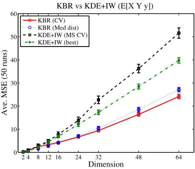
5.1 Nonparametric Inference of Posterior

The first numerical example is a comparison between KBR and a kernel density estimation (KDE) approach to obtaining conditional densities. Let (X1,Y1), . . . ,(Xn,Yn) be an i.i.d. sample from P on Rd_×Rr_{. With probability density functions K}X_{(x) on} Rd _andKY_{(y) on} Rr_{, the conditional} probability density functionp(y|x)is estimated by

b

p(y_|x) =∑

n

j=1KhXX(x−Xj)K

Y

hY(y−Yj)

∑nj=1KhX(x−Xj)

,

where K_hX

X(x) =h

−d

X KX(x/hX) andK_hY_Y(x) =hY−rKY(y/hY) (hX,hY >0). Given an i.i.d. sample U1, . . . ,Uℓfrom the prior Π, the particle representation of the posterior can be obtained by

impor-tance weighting (IW). Using this scheme, the posteriorq(x_|y)given y_∈Rr _{is represented by the} weighted sample(Ui,ζi)withζi=pb(y|Ui)/∑ℓj=1bp(y|Uj).

We compare the estimates of Rxq(x_|y)dx obtained by KBR and KDE + IW, using Gaussian

2 4 8 12 16 24 32 48 64 0

10 20 30 40 50 60

Dimension

Ave. MSE (50 runs)

KBR vs KDE+IW (E[X|Y=y])

KBR (CV) KBR (Med dist) KDE+IW (MS CV) KDE+IW (best)

Figure 2: Comparison between KBR and KDE+IW.

belong to the Gaussian kernel RKHS, hence the consistency result of Theorem 6 does not apply to

this function. In our experiments, the dimensionality was given byr=dranging from 2 to 64. The

distributionPof(X,Y)wasN((0,1_dT)T_{,V)withV =A}T_{A+2Id, where1}

d= (1, . . . ,1)T ∈Rd and each component ofAwas randomly generated asN(0,1)for each run. The priorΠwasN(0,VX X/2),

whereVX Xis theX-component ofV. The sample sizes weren=ℓ=200. The bandwidth parameters

hX,hY in KDE were sethX =hY, and chosen over the set_{2_∗i_|i=1, . . . ,10_} in two ways: least squares cross-validation (Rudemo, 1982; Bowman, 1984) and the best mean performance. For the KBR, we choseσine−kx−x′k2/(2σ2)in two ways: the median over the pairwise distances in the data (Gretton et al., 2008), and the 10-fold cross-validation approach described in Section 4.2. In the latter, σx forkX is first chosen withσy forkY set as the median distances, and thenσy is chosen

with the bestσx. Figure 2 shows the mean square errors (MSE) of the estimates over 1000 random

pointsy_∼N(0,VYY). KBR significantly outperforms the KDE+IW approach. Unsurprisingly, the

MSE of both methods increases with dimensionality.

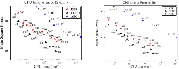
5.2 Bayesian Computation Without Likelihood

We compare ABC and the kernel methods, KBR and conditional mean, in terms of estimation accuracy and computational time, since they have an obvious tradeoff. To compute the estimation accuracy rigorously, the ground truth is needed: thus we use Gaussian distributions for the true prior and likelihood, which makes the posterior easy to compute in closed form. The samples are taken from the same model used in Section 5.1, andRxq(x_|y)dxis evaluated at 10 different values ofy.

We performed 10 runs with different randomly chosen parameter valuesA, representing the “true”

distributions.

For ABC, we used only the rejection method; while there are more advanced sampling schemes (Marjoram et al., 2003; Sisson et al., 2007), their implementation is dependent on the problem being

solved. Various values for the acceptance region τare used, and the accuracy and computational

time are shown in Fig. 3 together with total sizes of the generated samples. For the kernel methods, the sample sizen is varied. The regularization parameters are given byεn=0.01/nandδn=2εn

100 101 102 103 10-3

10-2

CPU time vs Error (2 dim.)

CPU time (sec)

Mean Square Errors

KBR COND ABC

6.1 102

1.5 103

2.1 105

4.9 103

2.7 103

3.1 104

8000 2000 1500 1000 800 600 400 200 3000 6000 4000 5000 200 400 600 800 1000 1500 2000 3000 4000 5000 6000

100 101 102 103 104

10-2 10-1

CPU time vs Error (6 dim.)

CPU time (sec)

Mean Square Errors

KBR COND ABC

3.3 102

1.3 106 7.0 104

1.0 104

2.5 103

9.5 102

200 400 2000 600 800 1500 1000 5000 6000 4000 3000 200 400 2000 4000 600 800 1000 1500 6000 3000 5000

Figure 3: Comparison of estimation accuracy and computational time with KBR and ABC for Bayesian computation without likelihood. COND reprensents the method based on Equa-tion (19). The numbers at the marks are the sample sizes generated for computaEqua-tion.

are Gaussian kernels for which the bandwidth parameters are chosen by the median of the pairwise distances on the data (Gretton et al., 2008). The incomplete Cholesky decomposition with tolerance 0.001 is employed for the low-rank approximation. The resulting ranks are, for instance, around

30 for N=200 and around 50 for N =6000 in the case of KBR dimension 2; around 180 for

N=200 and 1200 forN=6000 in the case of dimension 6. This implies considerable reduction of

computational time especially in the case of large sample sizes. The experimental results indicate that kernel methods achieve more accurate results than ABC at a given computational cost. The conditional kernel mean yields the best results, since in this instance, it is not necessary to correct for a difference in distribution betweenΠandPX. In the next experiment, however, this simplification

can no longer be made.

5.3 Filtering Problems

We next compare the KBR filtering method (proposed in Section 4.3) with EKF and UKF on syn-thetic data.

KBR has the regularization parametersεT,δT, and kernel parameters forkX andkY (e.g., the

bandwidth parameter for an RBF kernel). Under the assumption that a training sample is available, cross-validation can be performed on the training sample to select the parameters. By dividing the training sample into two, one half is used to estimate the covariance operators Equation (16) with a candidate parameter set, and the other half to evaluate the estimation errors. To reduce the search space and attendant computational cost, we used a simpler procedure, settingδT=2εT, and

Gaussian kernel bandwidthsβσX andβσY, whereσXandσY were the median of pairwise distances

200 400 600 800 1000 0.02

0.04 0.06 0.08 0.1 0.12 0.14 0.16

Training sample size

Mean square errors

KBR EKF UKF

200 400 600 800 0.05

0.06 0.07 0.08 0.09

Training data size

Mean square errors

KBR EKF UKF

Data (a) Data (b)

Figure 4: Comparisons with the KBR Filter and EKF. (Average MSEs and standard errors over 30 runs.) (a): dynamics with weak nonlinearity (b): dynamics with strong nonlinearity.

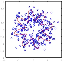
-2 -1 0 1 2

-2 -1.5 -1 -0.5 0 0.5 1 1.5 2

Figure 5: Example of data (b) (Xt,N=300)

Xt = (ut,vt)T∈R2, and the dynamics were given by

ut+1 vt+1

= (1+bsin(Mθt+1))

cosθt+1 sinθt+1

+ζt, θt+1=θt+η (mod 2π),

whereη>0 is an increment of the angle andζt ∼N(0,σ2_hI2) is independent process noise. Note that the dynamics of(ut,vt)were nonlinear even forb=0. The observationYt was

Yt= (ut,vt)T+ξt, ξt∼N(0,σ2oI),

whereξt was independent noise. The two dynamics were defined as follows: (a) rotation with noisy

observationsη=0.3,b=0,σh=σo=0.2; (b) oscillatory rotation with noisy observationsη=0.4, b=0.4,M=8,σh=σo=0.2. (See Fig.5). We assumed the correct dynamics were known to the EKF and UKF.

Results are shown in Fig. 4. In all cases, the EKF and UKF show an indistinguishably small difference. The dynamics in (a) are weakly nonlinear, and KBR has slightly worse MSE than EKF and UKF. For data set (b), which has strong nonlinearity, KBR outperforms the nonlinear Kalman filter forT _≥200.

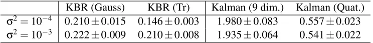
KBR (Gauss) KBR (Tr) Kalman (9 dim.) Kalman (Quat.) σ2₌₁₀−4 _{0.210±0.015 0.146±0.003 1.980±0.083 0.557±0.023} σ2₌₁₀−3 _{0.222±0.009 0.210±0.008 1.935±0.064 0.541±0.022} Table 1: Average MSE and standard errors for camera angle estimation (10 runs).

hidden variable, and movie frames recorded by the camera were observed. The data were generated virtually using a computer graphics environment. As in Song et al. (2009), we were given 3600 downsampled frames of 20_×20 RGB pixels (Yt _∈[0,1]1200_{), where the first 1800 frames were used} for training, and the second half were used to test the filter. We made the data noisy by adding Gaussian noiseN(0,σ2_)toYt.

Our experiments covered two settings. In the first, we did not use that the hidden state St

was included in SO(3), but only that it was a general 3_×3 matrix. In this case, we formulated the Kalman filter by estimating the relations under a linear assumption, and the KBR filter with Gaussian kernels forSt andXtas Euclidean vectors. In the second setting, we exploited the fact that St ∈SO(3): for the Kalman filter,St was represented by a quanternion, which is a standard vector representation of rotations; for the KBR filter the kernelk(A,B) =Tr[ABT]was used forSt, andSt

was estimated withinSO(3). Table 1 shows the Frobenius norms between the estimated matrix and

the true one. The KBR filter significantly outperforms the EKF, since KBR is able to extract the complex nonlinear dependence between the observation and the hidden state.

6. Proofs

This section includes the proofs of the theoretical results in Section 3.2. The proof ideas are similar to Caponnetto and De Vito (2007) and Smale and Zhou (2007), in which the basic techniques are taken from the general theory of regularization (Engl et al., 2000). Before stating the main proofs, we provide a proof of consistency of the empirical counterparts in Proposition 3 to the kernel Sum rule (Theorem 2). We then proceed to the proofs of Theorems 5 and 6, covering the consistency of

the KBR procedure in RKHS, followed by a proof of Theorem 7 for consistency inL2.

6.1 Consistency of the Kernel Sum Rule

We show consistency of an empirical estimate ofmQY in Theorem 2. The same proof also applies

in establishing consistency for the empirical estimatesCb_WW(n) andCb_{W Z}(n) in Proposition 3.

Theorem 8 Assume that CX X is injective, m_bΠ is a consistent estimator of mΠ in

H

X norm, and

that E[kY(Y,Y˜)|X =x,X˜ =x˜]is included in

H

X⊗

H

X as a function of (x,x˜), where (X˜,Y˜)is an

independent copy of (X,Y). Then, if the regularization coefficient εn decays to zero sufficiently slowly,

bC_{Y X}(n) Cb_{X X}(n)+εnI−1mbΠ−mQY _H

Y →0

in probability as n_→∞.

Proof The assertion is proved if, asn→∞,

in probability and

kCY X(CX X+εnI)−1mΠ−mQYkHY →0 (21)

with an appropriate choice ofεn.

By using the fact thatB−1₋A−1=B−1(A₋B)A−1holds for any invertible operatorsAandB, the left hand side of Equation (20) is upper bounded by

bC_{Y X}(n) Cb(_{X X}n)+εnI

−1

b

mΠ−mΠ_HY + bCY X(n)−CY X

CX X+εnI

−1 mΠ_HY

+ bC_{Y X}(n) Cb_{X X}(n)+εnI

−1

CX X−CbX X(n)

CX X+εnI

−1

mΠ_HY. (22)

By the decomposition

b

C_{Y X}(n)=Cb_YY(n)1/2Wb_{Y X}(n)Cb_{X X}(n)1/2 with_kWb_{Y X}(n)_{k ≤}1 (Baker, 1973), we have

kCb_{Y X}(n)(Cb_{X X}(n)+εnI)−1k ≤ kCb(n) 1/2 YY Wb

(n)

Y X(Cb

(n)

X X+εnI)−1/2k=Op(ε− 1/2 n ),

which implies the first term is ofOp(ε− 1/2

n kmbΠ−mΠkHX). From the

√

n-consistency of the

co-variance operators, the second and third terms are of the orderOp(n−1/2εn−1)andOp(n−1/2ε− 3/2 n ), respectively. Ifεnis taken so thatεn≫n−1/3andεn≫ kmb(Πn)−mΠk2_HX, Equation (20) converges to

zero in probability.

For Equation (21), first note

kCY X(CX X+εnI)−1mΠ−mQYk

2

HY

=_kCY X(CX X+εnI)−1mΠk2HX−2hCY X(CX X+εnI)

−1_m

Π,mQYiHY +kmQYk

2

HY.

Letθ(x,x˜):=E[kY(Y,Y˜)|X=x,X˜ =x˜]. The third term in the right hand side is

hmQY,mQYiHY =

Z Z

mQY(y)dPY|x(y)dΠ(x)

=

Z Z

hmQY,kY(·,y)iHYdPY|x(y)dΠ(x) =

Z Z

θ(x,x˜)dΠ(x)dΠ(x˜).

From the assumptionθ_∈

H

X⊗

H

X and the factE[mQY(Y)|X=·] =

R

θ(_·,x˜)dΠ(x˜), Lemma 9 below showsE[mQY(Y)|X =·]∈

H

X. It follows from Theorem 1 thatCXYmQY =CX XE[mQY(Y)|X =·]

and thus

hCY X(CX X+εnI)−1mΠ,mQYiHY =hmΠ,(CX X+εnI)

−1_CXYmQ

YiHX

=_hmΠ,(CX X+εnI)−1CX XE[mQY(Y)|X=·]iHX,

which converges to

hmΠ,E[mQY(Y)|X=·]iHX =

Z Z

θ(x,x˜)dΠ(x)dΠ(x˜)

Note that

kCY Xf_k2_H

Y =hCY Xf,CY XfiHX =E[f(X)(CY Xf)(Y)]

=E[f(X)E[kY(Y,Y˜)f(X˜)]] =E[f(X)f(X˜)θ(X,X˜)]

for any f ∈

H

X, where(X˜,Y˜)is an independent copy of(X,Y). By taking f = (CX X+εnI)−1mΠ,

the first term is given by

Eθ(X,X˜)((CX X+εnI)−1mΠ)(X)((CX X+εnI)−1mΠ)(X˜) =Eθ(X,_X˜_)f(X)f(X˜₎

=θ,(CX X⊗CX X)f⊗f)

HX⊗HX

=θ,(CX X(CX X+εnI)−1mΠ)⊗(CX X(CX X+εnI)−1mΠ)_HX⊗HX,

which, by Lemma 10, converges to

hθ,mΠ⊗mΠiHX⊗HX =

Z Z

θ(x,x˜)dΠ(x)dΠ(x˜).

This completes the proof.

Lemma 9 Let

H

X and

H

Y be RKHS’s on

X

and

Y

, respectively. If a functionθon

X

×

Y

is in

H

X⊗

H

Y (product space), then for any fixed y∈

Y

the functionθ(·,y) of the first argument is in

H

X.

Proof Let_{φi}Ii=1and{ψj}Jj=1be complete orthonormal bases of

H

X and

H

Y, respectively, where I,J_∈N_{∪ {∞}. Thenθis expressed as}

θ=

I

∑

i=1 J

∑

j=1 αi jφiψj

with∑i,j|αi j|2<∞(e.g., Aronszajn, 1950). We haveθ(·,y) =∑Ii=1βiφi withβi=∑Jj=1αi jψj(y). Since

∑

i

|βi|2=

∑

i

∑

j

αi jψj(y)

2

≤

∑

i

∑

j

|αi j|2

∑

j

|ψj(y)|2=

∑

i j

|αi j|2

∑

j

hψj,kY(·,y)i2HY =

∑

i j

|αi j|2kkY(·,y)k2HY <∞,

we haveθ(_·,y)_∈

H

X.

Lemma 10 Let

H

be a separable Hilbert space and C be a positive, injective, self-adjoint, compact operator on

H

. then, for any f _∈

H

,

Proof By the assumptions, there exist an orthonormal basis_{φi}for

H

and positive eigenvaluesλi such that

C f =

_∑

i

λihf,φiiHφi.

Then, we have

k(C+εI)−1C f₋f_k2_H =

∑

i

_λ ε

i+ε

2|hf,φiiH|2.

Since(ε/λi+ε)

2

≤1 and∑i|hf,φiiH|2=kfk2H <∞, the dominated convergence theorem ensures

lim

ε→+0k(C+εI) −1_{C f}

−f_k2_H =

_∑

i lim

ε→+0

_λ ε

i+ε

2|hf,φiiH|2=0,

which completes the proof.

6.2 Consistency Results in RKHS Norm

We first prove Theorem 5.

Proof[Proof of Theorem 5] By replacingY _7→(X,Y)andY _7→(Y,Y), it follows from Theorem 8 thatCb_ZW(n) andCb_WW(n) are consistent estimators ofCZW andCWW, respectively, in operator norm. For the proof, it then suffices to show

bC_ZW(n) Cb_WW(n) 2+δnI

−1_b

C_WW(n) kY(·,y)−CZW(CWW2 +δnI)−1CWWkY(·,y) _H

X →0

in probability and

CZW(CWW2 +δnI)−1CWWkY(·,y)−mQX|y _H

X →0

with an appropriate choice of δn. The proof of the first convergence is similar to the proof of

Equation (20) in Theorem 8, and we omit it. The proof of the second convergence is also similar to Theorem 8. The square of the left hand side is decomposed as

CZW(CWW2 +δnI

−1

CWWkY(·,y) 2

HX

−2CZW(C_WW2 +δnI)−1CWWkY(·,y),mQX|y

HX+ mQX|y

2

HX.

Letξ_∈

H

_Y⊗

H

_Y be defined byξ(y,y˜):=E[kX(Z,Z˜)|W =y,W˜ =y˜], where(Z˜,W˜)be an

indepen-dent copy of(Z,W). The third term is then equal to

ξ(y,y) =E[kX(Z,Z˜)|W=y,W˜ =y].

For the second term, by the same argument as the proof of Theorem 8, we have

ξ(y,_·) =E[kX(Z,Z˜)|W=y,W˜ =·]∈

H

Y

via Lemma 9, and

We then obtain

CZW(C_WW2 +δnI)−1CWWkY(·,y),mQX|y

HX =

kY(·,y),(CWW2 +δnI)−1CWW2 ξ(·,y)

HX,

which converges toξ(y,y).

Finally, definingϕδ:= (CWW2 +δI)−1CWWkY(·,y), the first term is equal to

Eϕ_δ(W)ϕ_δ(_W˜_)E[kX(Z,Z˜_)|W,W˜_{]=CZWϕδ,CZWϕδ}

HX =E h

ϕ_δ(W)CZWϕ_δ(Z)i

=Ek(Z,Z′)ϕ_δ(W)ϕ_δ(_W˜_)=Eξ(W,W˜_{)ϕδ(W)ϕδ(W}˜₎

=_h(CWW⊗CWW)ϕδ⊗ϕδ,ξiHY⊗HY =h(CWWϕδ)⊗(CWWϕδ),ξiHY⊗HY,

which converges to_hkY(·,y)⊗kY(·,y),ξiHY⊗HY =ξ(y,y). This completes the proof.

We next show the convergence rate of expectation (Theorem 6) under stronger assumptions. The first result is a rate of convergence for the mean transition in Theorem 2. In the following,

R

(C_{X X}0 )

means

H

X.

Theorem 11 Assume that the Radon-Nikodym derivative dΠ/dPX is included in

R

(C_{X X}β )for some

β_≥0, and letm_b(_Πn)be an estimator of mΠsuch thatkmbΠ(n)−mΠkHX =Op(n−

α_{)as n→∞for some}

0<α_≤1/2. Then, withεn=n−max{

2

3α,1+αβ}_{, we have}

bC_{Y X}(n) Cb(_{X X}n)+εnI

−1

b

m(_Πn)₋mQY _H

Y =Op(n

−min{2

3α,

2β+1

2β+2α}), (_n→∞).

Proof Takeη_∈

H

X such thatdΠ/dPX =C_{X X}β η. Then, we have

mΠ=

Z

kX(·,x) _dΠ

dPX

(x)dPX(x) =Cβ_{X X}+1η. (23)

First we show the rate of the estimation error:

bC_{Y X}(n) Cb_{X X}(n)+εnI−1m_b(_Πn)₋CY X CX X+εnI−1mΠ_H

Y =Op n

−α_ε−1/2 n

, (24)

asn_→∞. The left hand side of Equation (24) is upper bounded by

bC_{Y X}(n) Cb(_{X X}n)+εnI

−1

b

m(_Πn)₋mΠ_HY + bCY X(n)−CY X

CX X+εnI

−1 mΠ_HY

+ bC_{Y X}(n) Cb_{X X}(n)+εnI−1 CX X−Cb_{X X}(n) CX X+εnI−1mΠ_H Y.

In a similar manner to derivation of the bound of Equation (22), we obtain Equation (24). Next, we show the rate for the approximation error

CY X CX X+εnI

−1

mΠ−mQY _H

Y =O(ε

min_{(1+2β)/2,1_}

n ) (n→∞). (25)

LetCY X =C_YY1/2WY XCX X1/2be the decomposition withkWY Xk ≤1. It follows from Equation (23) and the relation

mQY =

Z Z

kY(·,y)dPY_|x(y)dΠ(x) = Z Z

k(_·,y)dΠ

dPX

(x)dPY_|x(y)dPX(x)

=

Z Z

k(_·,y)dΠ

dPX