A Bahadur Representation of the Linear Support Vector Machine

(1)

A Bahadur Representation of the Linear Support Vector Machine

Ja-Yong Koo [email protected]

Department of Statistics Korea University Seoul, 136-701, Korea

Yoonkyung Lee [email protected]

Department of Statistics The Ohio State University Columbus, OH 43210, USA

Yuwon Kim [email protected]

Data Mining Team NHN Inc.

Gyeonggi-do 463-847, Korea

Changyi Park [email protected]

Department of Statistics University of Seoul Seoul, 130-743, Korea

Editor: John Shawe-Taylor

Abstract

The support vector machine has been successful in a variety of applications. Also on the theoretical front, statistical properties of the support vector machine have been studied quite extensively with a particular attention to its Bayes risk consistency under some conditions. In this paper, we study somewhat basic statistical properties of the support vector machine yet to be investigated, namely the asymptotic behavior of the coefficients of the linear support vector machine. A Bahadur type representation of the coefficients is established under appropriate conditions, and their asymptotic normality and statistical variability are derived on the basis of the representation. These asymptotic results do not only help further our understanding of the support vector machine, but also they can be useful for related statistical inferences.

Keywords: asymptotic normality, Bahadur representation, classification, convexity lemma, Radon transform

1. Introduction

(2)

existing theoretical analysis of the SVM largely concerns its asymptotic risk, there are some basic statistical properties of the SVM that seem to have eluded our attention. For example, to the best of our knowledge, large sample properties of the coefficients in the linear SVM have not been studied so far although the magnitude of each coefficient is often the determining factor of feature selection for the SVM in practice.

In this paper, we address this basic question of the statistical behavior of the linear SVM as a first step to the study of more general properties of the SVM. We mainly investigate asymptotic properties of the coefficients of variables in the SVM solution for linear classification. The inves-tigation is done in the standard way that parametric methods are studied in a finite dimensional setting, that is, the number of variables is assumed to be fixed and the sample size grows to in-finity. Additionally, in the asymptotics, the effect of regularization through maximization of the class margin is assumed to vanish at a certain rate so that the solution is ultimately governed by the empirical risk. Due to these assumptions, the asymptotic results become more pertinent to the classical parametric setting where the number of features is moderate compared to the sample size and the virtue of regularization is minute than to the situation with high dimensional inputs. Despite the difference between the practical situation where the SVM methods are effectively used and the setting theoretically posited in this paper, the asymptotic results shed a new light on the SVM from a classical parametric point of view. In particular, we establish a Bahadur type representation of the coefficients as in the studies of sample quantiles and estimates of regression quantiles. See Bahadur (1966) and Chaudhuri (1991) for reference. It turns out that the Bahadur type representation of the SVM coefficients depends on Radon transform of the second moments of the variables. This representation illuminates how the so called margins of the optimal separating hyperplane and the underlying probability distribution within and around the margins determine the statistical behavior of the estimated coefficients. Asymptotic normality of the coefficients then follows immediately from the representation. The proximity of the hinge loss function that defines the SVM solution to the absolute error loss and its convexity allow such asymptotic results akin to those for least absolute deviation regression estimators in Pollard (1991).

In addition to providing an insight into the asymptotic behavior of the SVM, we expect that our results can be useful for related statistical inferences on the SVM, for instance, feature selection. For introduction to feature selection, see Guyon and Elisseeff (2003), and for an extensive empirical study of feature selection using SVM-based criteria, see Ishak and Ghattas (2005). In particular, Guyon, Weston, Barnhill, and Vapnik (2002) proposed a recursive feature elimination procedure for the SVM with an application to gene selection in microarray data analysis. Its selection or elimination criterion is based on the absolute value of a coefficient not its standardized value. The asymptotic variability of estimated coefficients that we provide can be used in deriving a new feature selection criterion which takes inherent statistical variability into account.

This paper is organized as follows. Section 2 contains the main results of a Bahadur type representation of the linear SVM coefficients and their asymptotic normality under mild conditions. An illustrative example is then provided in Section 3 followed by simulation studies in Section 4 and a discussion in Section 5. Proofs of technical lemmas and theorems are collected in Section 6.

2. Main Results

(3)

2.1 Preliminaries

Let(X,Y)be a pair of random variables with X ∈

X

⊂Rd _{and Y}_{∈ {}₁_,₋₁_}_{. The marginal} distri-bution of Y is given byP_(Y ₌₁_{) =}π₊ _andP_(Y ₌₋₁_{) =}π₋ _withπ₊_,π₋_>_{0 and}π₊₊π₋₌_1.

Let f and g be the densities of X given Y =1 and ₋1 with respect to the Lebesgue measure. Let _{(Xi_,Yi₎_}n

i=1 be a set of training data, independently drawn from the distribution of(X,Y). Denote the input variables as x= (x1, . . . ,xd)> and their coefficients as β+= (β1, . . . ,βd)>. Let

e

x= (_ex0, . . . ,exd)>= (1,x1, . . . ,xd)> andβ= (β0,β1, . . . ,βd)>. We consider linear classifications with hyperplanes defined by h(x;β) =β0+x>β+ =ex>β. Letk · k denote the Euclidean norm of a vector. For separable cases, the SVM finds the hyperplane that maximizes the geometric mar-gin, 2/_kβ+k2 _{subject to the constraints y}i_h(xi_;_β₎_≥_{1 for i}₌₁_{, . . . ,}_{n. For non-separable cases, a} soft-margin SVM is introduced to minimize

C

n

∑

i=1 ξi+

1 2kβ+k

2

subject to the constraints ξi ≥1−yih(xi;β) andξi≥0 for i=1, . . . ,n, where C>0 is a tuning parameter and_{ξi}ni=1are called the slack variables. Equivalently, the SVM minimizes the uncon-strained objective function

l_λ,n(β) = 1

n

∑

i=1

h

1₋yih(xi_;_β₎i

++ λ 2kβ+k

2 ₍₁₎

over β_∈Rd+1_{, where} _[z]₊ ₌_max_(z,₀₎ _{for z}_∈R _and λ_>_{0 is a penalization parameter; see}

Vapnik (1996) for details. Let the minimizer of (1) be denoted bybβ_λ,_n=arg min_βl_λ,_n(β). Note that

C= (nλ)−1_{. Choice of} λ_{depends on the data, and usually it is estimated via cross validation in} practice. In this paper, we consider only nonseparable cases and assume thatλ_→0 as n_→∞. We note that separable cases require a different treatment for asymptotics becauseλhas to be nonzero in the limit for the uniqueness of the solution.

Before we proceed with a discussion of the asymptotics of thebβ_λ,n, we introduce some notation and definitions first. The population version of (1) without the penalty term is defined as

L(β) =Eh₁₋_{Y h(X ;}β₎i

+ (2)

and its minimizer is denoted byβ∗ =arg min_βL(β). Then the population version of the optimal hyperplane defined by the SVM is

e

x>β∗=0. (3)

Sets are identified with their indicator functions. For example,

Z

Xxj{xj > 0}f(x)dx =

R

{x∈X : xj>0}xjf(x)dx. Lettingψ(z) ={z≥0}for z∈R, we define S(β) = (S(β)j)to be the(d+1)

-dimensional vector given by

S(β) =₋Eψ₍₁₋_{Y h(X ;}β_))Y_Xe

and H(β) = (H(β)jk)to be the(d+1)×(d+1)-dimensional matrix given by

(4)

whereδ denotes the Dirac delta function withδ(t) =ψ0_(t) _{in distributional sense. Provided that}

S(β)and H(β)are well-defined, S(β)and H(β)are considered as the gradient and Hessian matrix of L(β), respectively. Formal proofs of these relationships are given in Section 6.1.

For explanation of H(β), we introduce a Radon transformation. For a function s on

X

, define the Radon transform

R

s of s for p_∈R_andξ_∈Rd _as

(

R

s)(p,ξ) = Z

Xδ(p−ξ

>_x)s(x)dx.

For 0_≤ j,k_≤d, the(j,k)-th element of the Hessian matrix H(β)is given by

H(β)jk=π+(

R

fjk)(1−β0,β+) +π₋(

R

gjk)(1+β0,−β+), (4) where fjk(x) =exjxekf(x)and gjk(x) =exjexkg(x). Equation (4) shows that the Hessian matrix H(β) depends on the Radon transforms of fjk and gjk for 0≤ j,k≤d. For Radon transform and its properties in general, see Natterer (1986), Deans (1993), or Ramm and Katsevich (1996).

For a continuous integrable function s, it can be easily proved that

R

s is continuous. If f and g

are continuous densities with finite second moments, then fjkand gjkare continuous and integrable for 0_≤ j,k_≤d. Hence H(β)is continuous inβwhen f and g are continuous and have finite second moments.

2.2 Asymptotics

Now we present the asymptotic results forbβ_λ,n. We state regularity conditions for the asymptotics first. Some remarks on the conditions then follow for exposition and clarification. Throughout this paper, we use C1,C2, . . .to denote positive constants independent of n.

(A1) The densities f and g are continuous and have finite second moments.

(A2) There exists B(x0,δ0), a ball centered at x0with radiusδ0>0 such that f(x)>C1and g(x)>

C1for every x∈B(x0,δ0). (A3) For some 1_≤i∗_≤d,

Z

X{xi∗ ≥G

−

i∗}xi∗g(x)dx<

Z

X{xi∗ ≤F

+

i∗ }xi∗f(x)dx

or _Z

X{xi∗≤G

+

i∗}xi∗g(x)dx>

Z

X{xi∗ ≥F

−

i∗}xi∗f(x)dx.

Here F_i+∗ ,G+_i∗ ∈[−∞,∞]are upper bounds such that

Z

X{xi∗≤F

+

i∗ }f(x)dx=min

1,π−

π+

and

Z

X{xi∗ ≤G

+

i∗}g(x)dx=min

1,π+

π₋

. Similarly, lower bounds F_i−∗ and G−_i∗ are defined as

Z

X{xi∗ ≥F

−

i∗ }f(x)dx=min

1,π−

π+

and

Z

X{xi∗ ≥G

−

i∗}g(x)dx=min

1,π+

π₋

.

(A4) For an orthogonal transformation Aj∗ that mapsβ∗₊/kβ∗+kto the j∗-th unit vector e_j∗ for some 1_≤ j∗_≤d, there exist rectangles

D

+₌_{_x_∈_M+_{: l}

(5)

and

D

−₌_{_x_∈_M−_{: l}

i≤(Aj∗x)_i≤v_i with l_i<v_ifor i6= j∗}

such that f(x)_≥C2>0 on

D

+, and g(x)≥C3>0 on

D

−, where M+={x∈

X

|β∗₀+x>β∗+= 1_}and M−=_{x_∈

X

_|β₀∗+x>β∗₊=₋1_}.

Remark 1

• (A1) ensures that H(β)is well-defined and continuous inβ.

• When f and g are continuous, the condition that f(x0)>0 and g(x0)>0 for some x0implies

(A2).

• The technical condition in (A3) is a minimal requirement to guarantee thatβ∗₊, the normal vector of the theoretically optimal hyperplane is not zero. Roughly speaking, it says that for at least one input variable, the mean values of the class conditional distributions f and g have to be different in order to avoid the degenerate case ofβ∗₊=0. Some restriction of the

supports through F_i+∗ , G+_i∗, F_i−∗ and G−_i∗ is necessary in defining the mean values to adjust for

potentially unequal class proportions. Whenπ+=π₋, F_i+∗ and G+_i∗ can be taken to be+∞

and F_i−∗ and G−_i∗ can be−∞. In this case, (A3) simply states that the mean vectors for the two

classes are different.

• (A4) is needed for the positive-definiteness of H(β) around β∗. The condition means that there exist two subsets of the classification margins, M+and M−on which the class densities f and g are bounded away from zero. For mathematical simplicity, the rectangular subsets

D

+ _and

_D

− _{are defined as the mirror images of each other along the normal direction of}

the optimal hyperplane. This condition can be easily met when the supports of f and g are convex. Especially, ifRd _{is the support of f and g, it is trivially satisfied. (A4) requires that}

β∗

+6=0, which is implied by (A1) and (A3); see Lemma 4 for the proof. For the special case

d=1, M+and M−consist of a point.

D

+and

D

−are the same as M+and M−, respectively, and hence (A4) means that f and g are positive at those points in M+and M−.

Under the regularity conditions, we obtain a Bahadur-type representation of bβ_λ,n(Theorem 1). The asymptotic normality ofbβ_λ,nfollows immediately from the representation (Theorem 2). Con-sequently, we have the asymptotic normality of h(x;bβ_λ,n), the value of the SVM decision function at x (Corollary 3).

Theorem 1 Suppose that (A1)-(A4) are met. Forλ=o(n−1/2_{), we have} √

n(bβ_λ,_n₋β∗) =₋_√1 nH(β

∗₎−1

∑

n i=1

ψ(1−Yih(Xi_;_β∗_))Yi_X_ei₊_o P(1).

Theorem 2 Suppose (A1)-(A4) are satisfied. Forλ=o(n−1/2_), √

n(bβ_λ,n−β∗)→N

0,H(β∗)−1_G(_β∗_)H(_β∗₎−1

in distribution, where

(6)

Remark 2 Since bβ_λ,n is a consistent estimator of β∗ as n→∞, G(β∗) can be estimated by its

empirical version with β∗ replaced by bβ_λ,n. To estimate H(β∗), one may consider the following

nonparametric estimate:

1

n

" _n

∑

i=1

pb

1₋Yih(Xi;bβ_λ,n)

e

Xi(Xei)>

#

,

where pb(t)≡ p(t/b)/b, p(t)≥0 and

R

Rp(t)dt =1. Note that pb(·)→δ(·) as b→0. However,

estimation of H(β∗)requires further investigation.

Corollary 3 Under the same conditions as in Theorem 2,

√

nh(x;bβ_λ,n)−h(x;β∗)

→N0,x˜>H(β∗)−1_G(_β∗_)H(_β∗₎−1_x_˜

in distribution.

Remark 3 Corollary 3 can be used to construct a confidence bound for h(x;β∗₎_{based on an estimate}

h(x;bβ_λ,n), in particular, to judge whether h(x;β∗)is close to zero or not given x. This may be useful

if one wants to abstain from prediction at a new input x if it is close to the optimal classification boundary h(x;β∗) =0.

3. An Illustrative Example

In this section, we illustrate the relation between the Bayes decision boundary and the optimal hyperplane determined by (2) for two multivariate normal distributions inRd_{. Assume that f and g}

are multivariate normal densities with different mean vectors µf and µgand a common covariance matrixΣ. Suppose thatπ+=π₋=1/2.

We verify the assumptions (A1)-(A4) so that Theorem 2 is applicable. For normal densities f and g, (A1) holds trivially, and (A2) is satisfied with

C1 = |2πΣ|−1/2exp − sup kxk≤δ0

n

(x₋µf)>Σ−1(x−µf),(x−µg)>Σ−1(x−µg)

o!

forδ0>0. Since µf 6=µg, there exists 1≤i∗≤d such that i∗-th elements of µf and µgare different. By taking F_i∗+=G+_i∗ = +∞and F_i−∗ =G−_i∗ =−∞, we can show that one of the inequalities in (A3) holds as mentioned in Remark 1. Since

D

+and

D

−can be taken to be bounded sets of the form in (A4) inRd−1_{, and the normal densities f and g are bounded away from zero on such}

D

+ _and

D

−_,

(A4) is satisfied. In particular,β∗₊₆=0 as implied by Lemma 4.

Denote the density and cumulative distribution function of N(0,1) as φand Φ, respectively. Note thatβ∗should satisfy the equation S(β∗) =0, or

Φ(af) =Φ(ag) (5)

and

(7)

where af =

1₋β∗₀₋µ>_fβ∗₊

kΣ1/2β∗_+k , ag=

1+β∗₀+µ>_gβ∗₊

kΣ1/2β∗_+k andω∗=Σ1/2β∗+/kΣ1/2β∗+k. From (5) and the definition of af and ag, we have a∗≡af =ag. Hence

(β∗₊)>(µf+µg) =−2β∗0. (7)

It follows from (6) that

β∗

+/kΣ1/2β∗+k= Φ(a∗)

2φ(a∗₎Σ− 1_(µ

f−µg). (8)

First we show the existence of a proper constant a∗satisfying (8) and its relationship with a statisti-cal distance between the two classes. Defineϒ(a) =φ(a)/Φ(a)and let d_Σ(u,v) =_{(u₋v)>Σ−1_(u₋

v)_}1/2_{denote the Mahalanobis distance between u and v}_∈_Rd_{. Since}_kω∗_k₌_{1, we have}_ϒ_(a∗_{) =} kΣ−1/2_(µ

f−µg)k/2. Sinceϒ(a)is monotonically decreasing in a, there exists a∗=ϒ−1(dΣ(µf,µg)/2) that depends only on µf, µg, andΣ. For illustration, when the Mahalanobis distances between the two normal distributions are 2 and 3, a∗ is given by ϒ−1₍₁₎_{≈ −}₀_._{303 and}ϒ−1₍₁_.₅₎_{≈ −}₀_._969, respectively. The corresponding Bayes error rates are about 0.1587 and 0.06681. Figure 1 shows a graph ofϒ(a)and a∗when d_Σ(µf,µg)=2 and 3.

−3 −2 −1 0 1 2 3

0.0

0.5

1.0

1.5

2.0

2.5

3.0

a

Υ

(

a

)

Figure 1: A plot ofϒfunction. The dashed lines correspond to the inverse mapping from the Ma-halanobis distances of 2 and 3 to a∗_{≈ −}0.303 and₋0.969, respectively.

Once a∗is properly determined, we can express the solutionβ∗explicitly by (7) and (8):

β∗ 0=−

(8)

and

β∗ +=

2Σ−1(µf−µg) 2a∗dΣ(µf,µg) +dΣ(µf,µg)2

.

Thus the optimal hyperplane (3) is

2

2a∗dΣ(µf,µg) +dΣ(µf,µg)2

n

Σ−1_(µ f−µg)

o_>n

x₋1

2(µf+µg)

o

=0,

which is equivalent to the Bayes decision boundary given by

n

Σ−1_(µ f−µg)

o>n

x₋1

2(µf+µg)

o

=0.

This shows that the linear SVM is equivalent to Fisher’s linear discriminant analysis in this setting. In addition, H(β∗₎_{and G}₍_β∗₎_{can be shown to be}

G(β∗) =Φ(a∗)

2

2 (µf+µg)>

µf+µg G22(β∗)

and

H(β∗) = φ(a∗)

4 (2a ∗₊_d

Σ(µf,µg))

2 (µf+µg)>

µf+µg H22(β∗)

,

where

G22(β∗) = µfµ>f +µgµ>g +2Σ−

a∗ dΣ(µf,µg)

+1

(µf−µg)(µf−µg)>and

H22(β∗) = µfµ>f +µgµ>g +2Σ

+2 a

∗

d_Σ(µf,µg)

2

+ a∗

d_Σ(µf,µg)− 1

d2_Σ(µf,µg)

!

(µf−µg)(µf−µg)>.

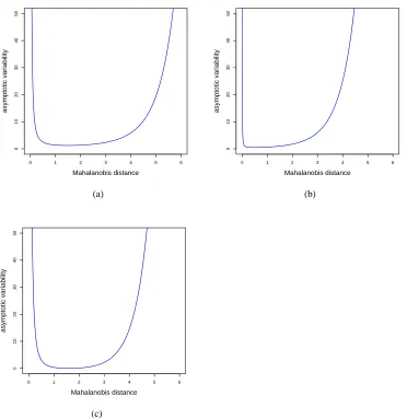
For illustration, we consider the case when d=1, µf+µg=0, and σ=1. The asymptotic variabilities of the intercept and the slope for the optimal decision boundary are calculated according to Theorem 2. Figure 2 shows the asymptotic variabilities as a function of the Mahalanobis distance between the two normal distributions,_|µf−µg|in this case. Also, it depicts the asymptotic variance of the estimated classification boundary value (−βˆ0/βˆ1) by using the delta method. Although the Mahalanobis distance roughly in the range of 1 to 4 would be of practical interest, the plots show a notable trend in the asymptotic variances as the distance varies. When the two classes get very close, the variances shoot up due to the difficulty in discriminating them. On the other hand, as the Mahalanobis distance increases, that is, the two classes become more separated, the variances become increasingly large. A possible explanation for the trend is that the intercept and the slope of the optimal hyperplane are determined by only a small fraction of data falling into the margins in this case.

4. Simulation Studies

(9)

0 1 2 3 4 5 6

0

10

20

30

40

50

Mahalanobis distance

asymptotic variability

(a)

0 1 2 3 4 5 6

0

10

20

30

40

50

(b)

0 1 2 3 4 5 6

0

10

20

30

40

50

(c)

Figure 2: The asymptotic variabilities of estimates of (a) the intercept, (b) the slope, and (c) their ratio for the optimal hyperplane as a function of the Mahalanobis distance.

4.1 Bivariate Case

Theorem 2 is numerically illustrated with the multivariate normal setting in the previous section. Consider a bivariate case with mean vectors µf = (1,1)> and µg= (−1,−1)> and a common co-variance matrixΣ=I2. This example has dΣ(µf,µg) =2

√

(10)

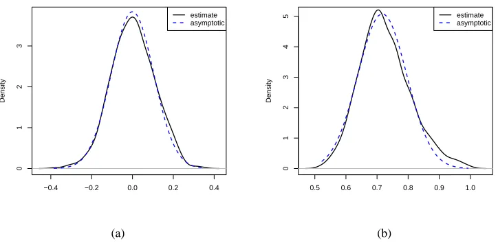
size, and Table 1 summarizes the results by showing the averages of the estimated coefficients of the SVM over 1,000 replicates. As expected, the averages get closer to the theoretically optimal coefficientsβ∗ as the sample size grows. Moreover, the sampling distributions of ˆβ0, ˆβ1, and ˆβ2 approximate their theoretical counterparts for a large sample size as shown in Figure 3. The solid lines are the estimated density functions of ˆβ0 and ˆβ1 for n=500, and the dotted lines are the corresponding asymptotic normal densities in Theorem 2.

Coefficients Sample size n Optimal values 100 200 500

β0 0.0006 -0.0013 0.0022 0 β1 0.7709 0.7450 0.7254 0.7169 β2 0.7749 0.7459 0.7283 0.7169

Table 1: Averages of estimated and optimal coefficients over 1,000 replicates.

−0.4 −0.2 0.0 0.2 0.4

0

1

2

3

Density

estimate asymptotic

(a)

0.5 0.6 0.7 0.8 0.9 1.0

0

1

2

3

4

5

Density

estimate asymptotic

(b)

Figure 3: Estimated sampling distributions of (a) ˆβ0and (b) ˆβ1with the asymptotic normal densities overlaid.

4.2 Feature Selection

(11)

We investigate the possibility of using the standardized coefficients of ˆβfor selection of vari-ables. For practical applications, one needs to construct a reasonable nonparametric estimator of the asymptotic variance-covariance matrix, whose entries are defined through line integrals. A sim-ilar technical issue arises in quantile regression. See Koenker (2005) for some suggested variance estimators in the setting.

For the sake of simplicity in the second set of simulation, we used the theoretical asymptotic variance in standardizing ˆβand selected those variables with the absolute standardized coefficient exceeding a certain critical value. And we mainly monitored the type I error rate of falsely declaring the significance of a variable when it is not, over various settings of a mixture of two multivariate normal distributions. Different combinations of the sample size (n) and the number of variables (d) were tried. For a fixed even d, we set µf = (1d/2,0d/2)>, µg=0>_d, andΣ=Id, where 1pand

0p indicate p-vectors of ones and zeros, respectively. Thus only the first half of the d variables have nonzero coefficients in the optimal hyperplane of the linear SVM. Table 2 shows the minima, median, and maxima of such type I error rates in selection of relevant variables over 200 replicates when the critical value was z0.025≈1.96 (5% level of significance). If the asymptotic distributions were accurate, the error rates would be close to the nominal level of 0.05. On the whole, the table suggests that when d is small, the error rates are very close to the nominal level even for small sample sizes, while for a large d, n has to be quite large for the asymptotic distributions to be valid. This pattern is clearly seen in Figure 4, which displays the median values of the type I error rates. In passing, we note that changing the proportion of relevant variables did not seem to affect the error rates, which are not shown here.

Number of variables (d)

n 6 12 18 24

250 [0.050, 0.060, 0.090] [0.075, 0.108, 0.145] [0.250, 0.295, 0.330] [0.665, 0.698, 0.720] 500 [0.045, 0.080, 0.090] [0.040, 0.068, 0.095] [0.105, 0.130, 0.175] [0.275, 0.293, 0.335] 750 [0.030, 0.055, 0.070] [0.035, 0.065, 0.090] [0.055, 0.095, 0.115] [0.135, 0.185, 0.205] 1000 [0.050 ,0.065, 0.065] [0.060, 0.068, 0.095] [0.040, 0.075, 0.095] [0.105, 0.135, 0.175] 1250 [0.065, 0.065, 0.070] [0.035, 0.045, 0.050] [0.055, 0.080, 0.105] [0.070, 0.095, 0.125] 1500 [0.035, 0.050, 0.065] [0.040, 0.058, 0.085] [0.055, 0.075, 0.090] [0.050, 0.095, 0.135] 1750 [0.030, 0.035, 0.060] [0.035, 0.045, 0.075] [0.040, 0.065, 0.095] [0.055, 0.080, 0.120] 2000 [0.035, 0.040, 0.060] [0.040, 0.065, 0.080] [0.060, 0.070, 0.100] [0.055, 0.075, 0.105]

Table 2: The minimum, median, and maximum values of the type I error rates of falsely flagging an irrelevant variable as relevant over 200 replicates by using the standardized SVM coef-ficients at 5% significance level.

We leave further development of asymptotic variance estimators for feature selection and com-parison with risk based approaches such as the recursive feature elimination procedure as a future work.

5. Discussion

(12)

500 1000 1500 2000

0.0

0.1

0.2

0.3

0.4

0.5

0.6

0.7

n

Type I error rate

d=6 d=12 d=18 d=24

Figure 4: The median values of the type I error rates in variable selection depending on the sample size n and the number of variables d. The horizontal, dashed line indicates the nominal level of 0.05.

type representation of the coefficients and their asymptotic normality using Radon transformation of the second moments of the variables. The representation shows how the statistical behavior of the coefficients is determined by the margins of the optimal hyperplane and the underlying probability distribution. Shedding a new statistical light on the SVM, these results provide an insight into its asymptotic behavior and can be used to improve our statistical practice with the SVM in various aspects.

(13)

char-acterization of which bears a close resemblance with function estimation for the nonlinear case. However, the theory was developed under the assumption of the differentiability of the loss, and it has to be modified for proper theoretical analysis of the SVM. As in the approach for the linear case presented in this paper, one may get around the non-differentiability issue of the hinge loss by imposing appropriate regularity conditions to ensure that the minimizer is unique and the expected loss is differentiable and locally quadratic around the minimizer.

Consideration of these extensions will lead to a more complete picture of the asymptotic behav-ior of the SVM solution.

6. Proofs

In this section, we present technical lemmas and prove the main results.

6.1 Technical Lemmas

Lemma 1 shows that there is a finite minimizer of L(β), which is useful in proving the uniqueness of the minimizer in Lemma 6. In fact, the existence of the first moment of X is sufficient for Lemmas 1, 2, and 4. However, (A1) is needed for the existence and continuity of H(β)in the proof of other lemmas and theorems.

Lemma 1 Suppose that (A1) and (A2) are satisfied. Then L(β)_→∞as_kβ_{k →}∞and the existence ofβ∗is guaranteed.

Proof. Without loss of generality, we may assume that x0=0 in (A2) and B(0,δ0)⊂

X

. For any ε>0,

L(β) = π+

Z

X[1−xe

>_β_]

+f(x)dx+π−

Z

X[1+h(x;β)]+g(x)dx

≥ π+

Z

X{h(x;β)≤0}(1−h(x;β))f(x)dx+π−

Z

X{h(x;β)≥0}(1+h(x;β))g(x)dx

≥ π+

Z

X{h(x;β)≤0}(−h(x;β))f(x)dx+π−

Z

X{h(x;β)≥0}h(x;β)g(x)dx

≥

Z

X|h(x;β)|min(π+f(x),π−g(x))dx

≥ C1min(π+,π−)

Z

B(0,δ0)

|h(x;β)_|dx

= C1min(π+,π−)kβk

Z

B(0,δ0)

|h(x; w)_|dx

≥ C1min(π+,π₋)kβkvol({|h(x; w)| ≥ε} ∩B(0,δ0))ε,

(14)

Note that−1≤w0≤1. For 0≤w0<1 and 0<ε<1, vol(_{|h(x; w)_{| ≥}ε_{} ∩}B(0,δ0)) ≥ vol(_{h(x; w)_≥ε_{} ∩}B(0,δ0))

= vol

x>w+/

q

1₋w2₀_≥(ε₋w0)/

q

1₋w2₀

∩B(0,δ0)

≥ vol

x>w+/

q

1₋w2₀_≥ε

∩B(0,δ0)

≡V(δ0,ε)

since(ε₋w0)/

q

1−w2₀≤ε. When−1<w0<0, we obtain volB(h(x; w)≤ −ε)≥V(δ0,ε)

in a similar way. Note that V(δ0,ε)is independent ofβand V(δ0,ε)>0 for someε<δ0. Conse-quently, L(β)_≥C1min(π+,π₋)kβkV(δ0,ε)ε→∞ as kβk →∞.The case w0=±1 is trivial.

Since the hinge loss is convex, L(β) is convex in β. Since L(β)_→∞ as _kβ_{k →}∞, the set, denoted by

M

, of minimizers of L(β)forms a bounded connected set. The existence of the solution

β∗_{of L}₍_β₎_{easily follows from this.}

In Lemmas 2 and 3, we obtain explicit forms of S(β)and H(β)for non-constant decision func-tions.

Lemma 2 Assume that (A1) is satisfied. Ifβ+₆=0, then we have

∂L(β)

∂βj

=S(β)j

for 0_≤ j_≤d.

Proof. It suffices to show that ∂ ∂βj

Z

X[1−h(x;β)]+f(x)dx=−

Z

X{h(x;β)≤1}xejf(x)dx.

Define∆(t) = [1₋h(x;β)₋t_exj]+−[1−h(x;β)]+. Let t>0. First, consider the casex_ej>0. Then,

∆(t) =

  

0 if h(x;β)>1

h(x;β)₋1 if 1₋tx_ej<h(x;β)≤1

−tx_ej if h(x;β)≤1−texj.

Observe that

Z

X∆(t){exj>0}f(x)dx =

Z

X{1−texj<h(x;β)≤1}(h(x;β)−1)f(x)dx

−t Z

X{h(x;β)≤1−texj,exj>0}exjf(x)dx

and that

1

t Z

X{1−texj<h(x;β)≤1}(h(x;β)−1)f(x)dx

≤

Z

(15)

By Dominated Convergence Theorem,

lim t↓0

Z

X{1−txej<h(x;β)≤1}exjf(x)dx=

Z

X{h(x;β) =1}xejf(x)dx=0

and

lim t↓0

Z

X{h(x;β)≤1−texj,exj>0}xejf(x)dx=

Z

X{h(x;β)≤1,xej>0}exjf(x)dx.

Hence

lim t↓0

1

t Z

X∆(t){exj>0}f(x)dx=−

Z

X{h(x;β)≤1,exj>0}xejf(x)dx. (9)

Now assume that_exj<0. Then,

∆(t) =

  

0 if h(x;β)>1₋t_exj 1−h(x;β)₋t_exj if 1<h(x;β)≤1−texj

−tx_ej if h(x;β)≤1.

In a similar fashion, one can show that

lim t↓0

1

t Z

X∆(t){exj<0}f(x)dx=−

Z

X{h(x;β)≤1,exj<0}xejf(x)dx. (10)

Combining (9) and (10), we have shown that

lim t_↓0

1

t Z

X∆(t)f(x)dx=−

Z

X{h(x;β)≤1}xejf(x)dx.

The proof for the case t<0 is similar.

The proof of Lemma 3 is based on the following identity

Z

δ(Dt+E)T(t)dt= 1

|D_|T(−E/D) (11)

for constants D and E. This identity follows from the fact thatδ(at) =δ(t)/_|a|andRδ

(t₋a)T(t)dt= T(a)for a constant a.

Lemma 3 Suppose that (A1) is satisfied. Under the condition thatβ+₆=0, we have

∂2_L(_β₎ ∂βj∂βk

=H(β)jk,

for 0_≤ j,k_≤d.

Proof. Define

Ψ(β) = Z

X{x

>_β+_<₁₋_β

0}s(x)dx

for a continuous and integrable function s defined on

X

. Without loss of generality, we may assume thatβ16=0. It is sufficient to show that for 0≤ j,k≤d,

∂2 ∂βj∂βk

Z

X[1−h(x;β)]+f(x)dx=

Z

(16)

Define

X

₋j={(x1, . . . ,xj−1,xj+1, . . . ,xd) : (x1, . . . ,xd)∈

X

}and

X

j={xj : (x1, . . . ,xd)∈

X

}. Observe that

∂Ψ(β)

∂β0

=₋ 1

|β1|

Z

X−1

s

1₋h(x;β) +β1x1 β1

,x2, . . . ,xd

dx₋1 (12)

and that for k₆=1,

∂Ψ(β)

∂βk

=₋ 1

|β1|

Z

X−1

xks

1₋h(x;β) +β1x1 β1

,x2, . . . ,xd

dx₋1. (13)

Ifβp=0 for any p6=1, then

∂Ψ(β)

∂β1

=₋1−β0

β1|β1|

Z

X−1

s

1−β0 β1

,x2, . . . ,xd

dx₋1. (14)

If there is p₆=1 withβp6=0, then we have

∂Ψ(β)

∂β1

=₋ 1

|βp|

Z

X−p x1s

x1, . . . ,xp−1,

1₋h(x;β) +βpxp

βp

,xp+1, . . . ,xd

dx₋p. (15)

Choose D=β1, E=xe>β−β1x1−1, t=x1in (11). It follows from (13) and (15) that ∂Ψ(β)

∂βk

= ₋ 1

|β1|

Z

X−1

xks

1₋h(x;β) +β1x1 β1

,x2, . . . ,xd

dx₋1 (16)

= ₋

Z

X−1 Z

X1

xks(x)δ(h(x;β)−1)dx1dx−1

= ₋

Z

Xδ(1−h(x;β))xks(x)dx.

Similarly, we have

∂Ψ(β)

∂β0

=₋

Z

Xδ(1−h(x;β))s(x)dx (17)

by (12).

Choosing D=β1, E=β0−1, t=x1in (11), we have

Z

X1

δ(β1x1−1+β0)x1s(x)dx1= 1 |β1|

1₋β0 β1

s

1₋β0 β1

,x2, . . . ,xd

by (14). This implies (16) for k=1. The desired result now follows from (16) and (17).

The following lemma asserts that the optimal decision function is not a constant under the condition that the centers of two classes are separated.

Lemma 4 Suppose that (A1) is satisfied. Then (A3) implies thatβ∗₊₆=0.

Proof. Suppose that

Z

X{xi∗≥G

−

i∗}xi∗g(x)dx<

Z

X{xi∗ ≤F

+

i∗}xi∗f(x)dx (18)

in (A3). We will show that

min

β0

L(β0,0, . . .0)> min

β0,βi∗>0

(17)

implying thatβ∗₊6=0. Henceforth, we will suppressβ’s that are equal to zero in L(β). The popula-tion minimizer(β∗₀,β∗_i∗)is given by the minimizer of

L(β0,βi∗) = π+

Z

X[1−β0−βi∗xi∗]+f(x)dx+π−

Z

X[1+β0+βi∗xi∗]+g(x)dx.

First, consider the caseβi∗=0.

L(β0) =

  

π₋(1+β0), β0>1 1+ (π₋₋π+)β0, −1≤β0≤1 π+(1₋β0), β0<−1 with its minimum

min

β0

L(β0) =2 min(π+,π−). (20) Now consider the caseβi∗ >0, where

L(β0,βi∗) = π+

Z

X

xi∗≤ 1−β0

βi∗

(1₋β0−βi∗x_i∗)f(x)dx

+π₋ Z

X

xi∗ ≥−1−β0

βi∗

(1+β0+βi∗x_i∗)g(x)dx.

Letβe0denote the minimizer of L(β0,βi∗)for a givenβ_i∗. Note that∂L(β₀,β_i∗)/∂β₀is given as

∂L(β0,βi∗)

∂β0

(21)

= ₋π+

Z

X

xi∗ ≤1−β0

βi∗

f(x)dx+π₋ Z

X

xi∗ ≥−1−β0

βi∗

g(x)dx,

which is monotonic increasing inβ0with limβ0→−∞

∂L(β0,βi∗)

∂β0 → −π+ and limβ0→∞

∂L(β0,βi∗) ∂β0 →π−.

Henceβe0exists for a givenβi∗.

When π₋ <π+, we can easily check that F_i+∗ <∞and G_i−∗ =−∞. F_i+∗ and G−_i∗ may not be determined uniquely, meaning that there may exist an interval with probability zero. There is no significant change in the proof under the assumption that F_i+∗ and G−_i∗ are unique. Note that

1₋βe0 βi∗ ≤F

+

i∗

by definition of F_i+∗ and (21). Then,

−1₋βe0 βi∗ ≤F

+

i∗ − 2

βi∗ → −∞ as βi ∗ →0,

and

1₋βe0 βi∗ →F

+

i∗ as βi∗→0.

¿From (18),

π₋Z

Xxi∗g(x)dx<π+

Z

X{xi∗ ≤F

+

(18)

Now consider the minimum of L(βe0,βi∗)with respect toβ_i∗>0. From (21),

L(βe0,βi∗) (23)

= π+

Z

X

(

xi∗≤1−

e

β0 βi∗

)

(1₋βe0−βi∗x_i∗)f(x)dx

+π₋ Z

X

(

xi∗ ≥−1−

e

β0 βi∗

)

(1+βe0+βi∗x_i∗)g(x)dx

= 2π₋

Z

X

(

xi∗≥−1−

e

β0 βi∗

)

g(x)dx

+βi∗ π₋

Z

X

(

xi∗ ≥−1−

e

β0 βi∗

)

xi∗g(x)dx−π+

Z

X

(

xi∗ ≤1−

e

β0 βi∗

)

xi∗f(x)dx

!

By (22), it can be easily seen that the second term in (23) is negative for sufficiently smallβi∗ >0, implying

L(βe0,βi∗)<2π₋ for some β_i∗>0.

Ifπ₋>π+, then F_i+∗ =∞and G−_i∗ >−∞.Similarly, it can be checked that

L(βe0,βi∗)<2π+ for some β_i∗>0. Suppose thatπ₋=π+. Then it can be verified that

1₋βe0

βi∗ →∞ as βi ∗ →0,

and

−1₋βe0

βi∗ → −∞ as βi ∗→0.

In this case, L(eβ0,βi∗)<1.

Hence, under (18), we have shown that

L(βe0,βi∗)<1 for some β_i∗ >0.

This, together with (20), implies (19). For the second case in (A3), the same arguments hold with

βi∗ <0.

Note that (A1) implies that H is well-defined and continuous in its argument. (A4) ensures that

H(β)is positive definite aroundβ∗and thus we have a lower bound result in Lemma 5.

Lemma 5 Under (A1), (A3) and (A4),

β>_H(_β∗₎_β_≥_C 4kβk2,

(19)

Proof. Since the proof for the case d=1 is trivial, we consider the case d≥2 only. Observe that

β>_H(_β∗₎_β ₌ _E_δ₍₁₋_{Y h(X ;}_β∗_))h2_{(X ;}_β₎

= π+

Z

Xδ(1−h(x;β

∗_))h2_(x;_β₎_f_(x)dx₊_π −

Z

Xδ(1+h(x;β

∗_))h2_(x;_β_)g(x)dx

= π+(

R

h2f)(1₋β∗₀,β∗₊) +π₋(

R

h2g)(1+β∗₀,₋β∗₊) = π+(

R

h2f)(1₋β∗₀,β∗₊) +π₋(

R

h2g)(₋1₋β∗₀,β∗₊).

The last equality follows from the homogeneity of Radon transform.

Recall thatβ∗₊₆=0 by Lemma 4. Without loss of generality, we assume that j∗=1 in (A4). Let

A1β+=a= (a1, . . . ,ad)and z= (A1x)/kβ∗+k. Given u= (u2, . . . ,ud), let u∗=

(1−β∗

0)/kβ∗+k,u

. Define

Z

=_{z= (A1x)/kβ∗+k: x∈

X

}and

U

={u : uj=kβ∗+kzjfor j=2, . . . ,d,and z∈

Z

}. Note that detA1=1, du=kβ∗+kd−1dz2. . .dzd,

kβ∗+kA>₁z

_z

1=(1−β∗0)/kβ∗+k2

=A>₁

    

(1₋β∗₀)/_kβ∗_+k

kβ∗_+k_z₂ .. . kβ∗_+k_z_d

   

=A

> 1u∗

and

β0+kβ∗+ka>z

z1=(1−β∗0)/kβ∗+k2

= β0+kβ∗+k

a1(1−β∗0)/kβ∗+k2+ d

∑

j=2

ajzj

= β0+a1(1−β0∗)/kβ∗+k+kβ∗+k d

∑

j=2

ajzj.

Using the transformation A1, we have

(

R

h2f)(1₋β∗₀,β∗₊) =

Z

Zδ

1₋β∗₀_{− k}β_+k∗ (A1β∗+)>z

h2_kβ∗_+kA>₁z;βf_kβ∗_+kA>₁z_kβ∗_+kddz =

Z

Zδ

1₋β∗₀_{− k}β∗_+k2e>₁zβ0+kβ∗+k(A1β+)>z

2

f_kβ∗_+kA₁>z_kβ∗_+kddz =

Z

Zδ 1−β

∗

0− kβ∗+k2z1β0+kβ∗+ka>z

2

f_kβ∗_+kA₁>z_kβ∗_+kddz

= 1

kβ∗+k

Z

U

β0+a1(1−β∗0)/kβ∗+k+ d

∑

j=2

ajuj

2

(20)

The last equality follows from the identity (11). Let

D

_∗+=u : A>₁u∗∈

D

+ _{. By (A4), there exists} a constant C2>0 and a rectangle

D

_∗+on which f(A>₁u∗)_≥C2for u∈

D

_∗+. Then

(

R

h2f)(1−β∗0,β∗+)

≥ 1

kβ∗_+k

Z

D+

∗

β0+a1(1−β∗0)/kβ∗+k+ d

∑

j=2

ajuj

2

f(A>₁u∗)du

≥ 1

kβ∗_+k·C2

Z

D+

∗

β0+a1(1−β∗0)/kβ∗+k+ d

∑

j=2

ajuj

2

du

= 1

kβ∗_+k·C2·vol(

D

_∗+)Eu

β0+a1(1−β∗0)/kβ∗+k+ d

∑

j=2

ajUj

2

= 1

kβ∗+k·C2·vol(

D

+ ∗)

n

β0+a1(1−β∗0)/kβ∗+k+Eu d

∑

j=2

ajUj

2

+Vu(

d

∑

j=2

ajUj)

o

,

where Ujfor j=2, . . . ,d are independent and uniform random variables defined on

D

_∗+, andEuand

Vu_{denote the expectation and variance with respect to the uniform distribution.}

Letting mi= (li+vi)/2, we have

(

R

h2f)(1₋β∗₀,β∗₊) (24)

≥ 1

kβ∗_+k·C2·vol(

D

_∗+)

n

β0+a1(1−β∗0)/kβ∗+k+ d

∑

j=2

ajmj

2

+ min

2≤j≤d

Vu_(U_j₎

d

∑

j=2

a2_jo.

Similarly, it can be shown that

(

R

h2g)(₋1₋β∗₀,β∗₊) (25)

≥ 1

kβ∗_+k·C3·vol(

D

_∗−)

n

β0−a1(1+β∗0)/kβ∗+k+ d

∑

j=2

ajmj

2

+ min

2≤j≤d

Vu_(U_j₎

d

∑

j=2

a2_jo,

(21)

Combining (24)-(25) and letting C5=2/_kβ∗_+kminπ+C2·vol(

D

_∗+),π₋C3·vol(

D

_∗−)

and C6=

min1,min2_≤j_≤dVu(Uj)

, we have

β>_H(_β∗₎_β

≥ π+

kβ∗+k·C2·vol(

D

+ ∗)

n

β0+a1(1−β∗0)/kβ∗+k+ d

∑

j=2

ajmj

2

+ min

2≤j≤d

Vu_(U_j₎

d

∑

j=2

a2_jo

+ π−

kβ∗_+k·C3·vol(

D

∗−)

n

β0−a1(1+β∗0)/kβ∗+k+ d

∑

j=2

ajmj

2

+ min

2≤j≤d

Vu_(U_j₎

d

∑

j=2

a2_jo

≥ C5C6

n

β0+a1(1−β∗0)/kβ∗+k+ d

∑

j=2

ajmj

2

+β0−a1(1+β∗0)/kβ∗+k+ d

∑

j=2

ajmj

2

+2

d

∑

j=2

a2_jo/2

= C5C6

n

β0+a1(1−β∗0)/kβ∗+k

2

+β0−a1(1+β∗0)/kβ∗+k

2

+4β0−a1β∗0/kβ∗+k

d

∑

j=2

ajmj+2

d

∑

j=2

ajmj

2

+2

d

∑

j=2

a2_jo/2.

Note that

d

∑

j=2

ajmj

2

+2β0−a1β∗0/kβ∗+k

d

∑

j=2

ajmj

=

d

∑

j=2

ajmj+β0−a1β∗0/kβ∗+k

2

−β0−a1β∗0/kβ∗+k

2

and

β0+a1(1−β∗0)/kβ∗+k

2

+β0−a1(1+β∗0)/kβ∗+k

2

−2β0−a1β∗0/kβ∗+k

2

=2a2₁/_kβ∗_+k2_. Thus, the lower bound ofβ>H(β∗)βexcept for the constant C5C6allows the following quadratic form in terms ofβ0,a1, . . . ,ad. Let

Q(β0,a1, . . . ,ad) =a21/kβ∗+k2+

d

∑

j=2

ajmj+β0−a1β∗0/kβ∗+k

2

+

d

∑

j=2

a2_j.

Obviously Q(β0,a1, . . . ,ad)≥0 and Q(β0,a1, . . . ,ad) =0 implies that a1=. . .=ad=0 andβ0=0. Therefore Q is positive definite. Lettingν1>0 be the smallest eigenvalue of the matrix correspond-ing to Q, we have proved

β>_H(_β∗₎_β _≥ _C

5C6ν1(β20+ d

∑

j=1

a2_j) =C5C6ν1(β20+ d

∑

j=1 β2

j).

(22)

Lemma 6 Suppose that (A1)-(A4) are met. Then L(β)has a unique minimizer.

Proof. By Lemma 1, we may choose any minimizerβ∗∈

M

. By Lemma 4 and 5, H(β)is positive definite atβ∗. Then L(β)is locally strictly convex atβ∗, so that L(β) has a local minimum atβ∗. Hence the minimizer of L(β)is unique.

6.2 Proof of Theorems 1 and 2

For fixedθ_∈Rd+1_{, define}

Λn(θ) =n

l_λ,n(β∗+θ/

√

n)₋l_λ,n(β∗)

and

Γn(θ) =EΛn(θ).

Observe that

Γn(θ) =n L(β∗+θ/√n)−L(β∗)

+λ

2

kθ+k2₊₂√_n_β∗ +>θ+

.

By Taylor series expansion of L aroundβ∗, we have

Γn(θ) = 1 2θ

>_H(_e_β₎_θ₊λ 2

kθ+k2+2√nβ∗₊>θ+,

whereeβ=β∗_{+ (t/}√_n)_θ_{for some 0}_<_t_<_{1. Define D}_jk₍_α_{) =}_H(_β∗₊_α₎_jk₋_H(_β∗₎_jk_{for 0}_≤_j,k_≤

d. Since H(β)is continuous in β, there existsδ1>0 such that |Djk(α)|<ε1ifkαk<δ1 for any ε1>0 and all 0≤ j,k≤d. Then, as n→∞,

1 2θ

>_H(_e_β₎_θ₌1 2θ

>_H(_β∗₎_θ₊_o(₁_).

It is because for sufficiently large n such that_k(t/√n)θ_k<δ1,

θ>H(eβ)₋H(β∗)θ _≤

∑

j,k

|θj||θk|

Djk

t

√

nθ

≤ ε1

∑

j,k

|θj||θk| ≤2ε1kθk2.

Together with the assumption thatλ=o(n−1/2₎_{, we have} Γn(θ) =

1 2θ

>_H(_β∗₎_θ₊_o(₁_).

Define Wn=−∑ni=1ζiYiXei whereζi=

n

Yih(Xi_;_β∗₎_≤₁o_{. Then} _√1

nWnfollows asymptotically

N0,nG(β∗)by central limit theorem. Note that

(23)

Recall thatβ∗is characterized by S(β∗_{) =}_{0 implying the first part of (26). If we define}

Ri,n(θ) =

h

1₋Yih(Xi;β∗+θ/√n)i

+−

h

1₋Yih(Xi;β∗)i

++ζ

i_Yi_h(Xi_;_θ_/√_n),

then we see that

Λn(θ) =Γn(θ) +Wn>θ/

√

n+

n

∑

i=1

Ri,n(θ)−ERi,n(θ)

and

Ri,n(θ)

≤h(Xi_;_θ_)/√_n

Uh(Xi_;_θ_)/√_n

, (27)

where

U(t) =n1₋Yih(Xi_;_β∗₎_≤_to _for _t_∈R_.

To verify (27), letζ=_{a_≤1_}and R= [1₋z]+−[1−a]++ζ(z−a). If a>1, then R= (1−z){z≤ 1_}; otherwise, R= (z₋1)_{z>1_}. Hence,

R = (1₋z)_{a>1,z_≤1_}+ (z₋1)_{a<1,z>1_} (28) ≤ |z₋a_|{a>1,z_≤1_}+_|z₋a_|{a<1,z>1_}

= _|z₋a_|_{a>1,z_≤1_}+_{a<1,z>1_}

≤ |z₋a_|{|1₋a_{| ≤ |}z₋a_|}.

Choosing z=Yih(Xi_;_β∗₊_θ_/√_n)_{and a}₌_Yi_h(Xi_;_β∗₎_{in (28) yields (27).}

Since cross-product terms inE₍∑_i_(R_i_,_n₋E_R_i_,_n₎₎2_{cancel out, we obtain from (27) that for each}

fixedθ,

n

∑

i=1

E_|_R_i_,_n₍θ₎₋E_R_i_,_n₍θ₎_|2 _≤

n

∑

i=1

E _R_i_,_n₍θ₎2

≤

n

∑

i=1

E _h(Xi_;θ_)/√_n2_U _|_h(Xi_;θ_)/√_n_|

≤

n

∑

i=1

E

(1+_kXi_k2)_kθ_k2/n U

q

1+_kXi_k2_kθ_k_/√_n

= _kθ_k2E

(1+_kX_k2)U

q

1+_kX_k2_kθ_k_/√_n

.

(A1) implies thatE _k_X_k2_<∞_{. Hence, for any}ε_>_{0, choose C7}_{such that}E₍₁₊_k_X_k2₎_{k_X_k_>

C7}

<ε/2. Then

E

(1+_kXk2₎_Uq₁₊_k_X_k2_kθ_k_/√_n

≤ E₍₁₊_k_X_k2₎_{k_X_k_>_C₇_}_{+ (}₁_+C2₇₎P

U

q

1+C₇2_kθ_k/√n

(24)

By (A1), the distribution of X is not degenerate, which in turn implies that limt↓0P(U(t)) =0. We can take a large N such thatP

U

q

1+C₇2_kθ_k/√n

<ε/(2(1+C₇2))for n_≥N. This proves

that

n

∑

i=1

E_|_R_i_,_n₍θ₎₋E_R_i_,_n₍θ₎_|2_→₀

as n_→∞. Thus, for each fixedθ,

Λn(θ) = 1 2θ

>_H(_β∗₎_θ_+W> n θ/

√

n+o_P(1).

Letηn=−H(β∗)−1Wn/√n. By Convexity Lemma in Pollard (1991), we have

Λn(θ) = 1

2(θ−ηn)

>_H(_β∗₎₍_θ₋_η n)−

1 2η

>

nH(β∗)ηn+rn(θ),

where, for each compact set K inRd+1_,

sup

θ∈K|

rn(θ)| →0 in probability.

Because ηn converges in distribution, there exists a compact set K containing Bε, where Bε is a closed ball with centerηnand radiusεwith probability arbitrarily close to one. Hence we have

∆n= sup

θ∈Bε

|rn(θ)| →0 in probability. (29)

For examination of the behavior ofΛn(θ)outside Bε, considerθ=ηn+γv, withγ>εand v, a unit vector and a boundary pointθ∗=ηn+εv. By Lemma 5, convexity ofΛn, and the definition of

∆n, we have

ε

γΛn(θ) +

1−ε_γ

Λn(ηn) ≥ Λn(θ∗)

≥ 1₂(θ∗₋ηn)>H(β∗)(θ∗−ηn)− 1 2η

>

nH(β∗)ηn−∆n

≥ C4 2 ε

2₊_Λ

n(ηn)−2∆n,

implying that

inf kθ−ηnk>ε

Λn(θ)≥Λn(ηn) +

C4 2 ε

2 −2∆n

.

By (29), we can take∆nso that 2∆n<C4ε2/4 with probability tending to one. So the minimum ofΛncannot occur at anyθwithkθ−ηnk>ε. Hence, for eachε>0 andbθλ,n=√n(bβλ,n−β∗),

P_kbθ_λ,_n₋η_n_k_>ε_→₀_.

This completes the proof of Theorems 1 and 2.

Acknowledgments

(25)

References

R. R. Bahadur. A note on quantiles in large samples. Annals of Mathematical Statistics, 37:577–580, 1966.

P. L. Bartlett, M. I. Jordan, and J. D. McAuliffe. Convexity, classification, and risk bounds. Journal

of the American Statististical Association, 101:138–156, 2006.

G. Blanchard, O. Bousquet, and P. Massart. Statistical performance of support vector machines.

The Annals of Statistics, 36:489–531, 2008.

P. Chaudhuri. Nonparametric estimates of regression quantiles and their local Bahadur representa-tion. The Annals of Statistics, 19:760–777, 1991.

C. Cortes and V. Vapnik. Support-vector networks. Machine Learning, 20:273–297, 1995.

N. Cristianini and J. Shawe-Taylor. An Introduction to Support Vector Machines and Other

Kernel-based Learning Methods. Cambridge University Press, Cambridge, 2000.

S. R. Deans. The Radon Transform and Some of Its Applications. Krieger Publishing Company, Florida, 1993.

I. Guyon and A. Elisseeff. Introduction to variable and feature selection. Journal of Machine

Learning Research, 3:1157–1182, 2003.

I. Guyon, J. Weston, S. Barnhill, and V. Vapnik. Gene selection for cancer classification using support vector machines. Machine Learning, 46:389–422, 2002.

A. B. Ishak and B. Ghattas. An efficient method for variable selection using svm-based criteria. Preprint, Institut de Math´ematiques de Luminy, 2005.

R. Koenker. Quantile Regression. Econometric Society Monographs. Cambridge University Press, 2005.

Y. Lin. Some asymptotic properties of the support vector machine. Technical report 1029, Depart-ment of Statistics, University of Wisconsin-Madison, 2000.

Y. Lin. A note on margin-based loss functions in classification. Statististics and Probability Letters, 68:73–82, 2002.

F. Natterer. The Mathematics of Computerized Tomography. Wiley & Sons, New York, 1986.

D. Pollard. Asymptotics for least absolute deviation regression estimators. Econometric Theory, 7: 186–199, 1991.

A. G. Ramm and A. I. Katsevich. The Radon Transform and Local Tomography. CRC Press, Boca Raton, 1996.

B. Sch¨olkopf and A. Smola. Learning with Kernels - Support Vector Machines, Regularization,

(26)

J. C. Scovel and I. Steinwart. Fast rates for support vector machines using gaussian kernels. The

Annals of Statistics, 35:575–607, 2007.

X. Shen. On methods of sieves and penalization. The Annals of Statistics, 25:2555–2591, 1997.

I. Steinwart. Consistency of support vector machines and other regularized kernel machines. IEEE

Transactions on Information Theory, 51:128–142, 2005.

V. Vapnik. The Nature of Statistical Learning Theory. Springer, New York, 1996.