Effects of First-Order Reactant on MHD Turbulence at Four-Point Correlation

(1)

Published online January 30, 2015 (http://www.sciencepublishinggroup.com/j/acm) doi: 10.11648/j.acm.20150401.13

ISSN: 2328-5605 (Print); ISSN: 2328-5613 (Online)

Effects of first-order reactant on MHD turbulence at

four-point correlation

M. Abu Bkar Pk

*

, Abdul Malek, M. Abul Kalam Azad

Department of Applied Mathematics, University of Rajshahi, Rajshahi, Bangladesh

Email address:

[email protected] (M. A. B. Pk), [email protected] (A. Malek), [email protected] (M. A. K. Azad)

To cite this article:

M. Abu Bkar Pk, Abdul Malek, M. Abul Kalam Azad. Effects of First-Order Reactant on MHD Turbulence at Four-Point Correlation. Applied and Computational Mathematics. Vol. 4, No. 1, 2015, pp. 11-19. doi: 10.11648/j.acm.20150401.13

Abstract:

The purpose of this study is to determine the effect of first order reactant of MHD fluid turbulence for four-point correlations earlier than the ending phase. Three and four point correlation equations are obtained. The correlation equations are changed to spectral type by their Fourier-transform. By neglecting the quintuple correlations in comparison to the fourth order correlation terms. As a final point integrating the energy spectrum over all wave numbers and we obtained the energy decompose rule of MHD turbulence for magnetic field fluctuations due to the effect of first order reactant and the result has been shown graphically.

Keywords: Correlation Function, Deissler’s Method, First Order Chemical Reactant, Fourier-Transformation,

Navier-Stokes Equation, MHD Turbulence

1. Introduction

The introduction of the Chemical reactions occur in the gas phase, in solution in a variety of solvents, at gas-solid and other interfaces, in the liquid state, and in the solid state. Chemical kinetics deals with the rates of chemical reactions and with how the rates depend on factors such as concentration and temperature. Such studies are important in providing essential evidence as to the mechanisms of chemical processes. Chemical reactions occur in solution in a variety of solvents, at gas-solid and other interfaces, in the liquid state. Here we apply on MHD turbulence. Deissler (1958, 1960) developed “A theory decay of homogeneous turbulence for times before the final period”. Using Deissler’s theory Kumar and Patel (1974) first order reactant in homogeneous turbulence before the final period of decay consideration. Kumar and Patel also discussed (1975) the first order reactant in homogeneous turbulence before the final period for the case of multi-point and multi-time. Sarker and Kishore (1991) studied the decay of MHD turbulence before the final periods. Bkar Pk et al (2012) studied the decay of energy of MHD turbulence for four point correlation. Islam and Sarker (2001) discussed the first- order reactant in MHD turbulence before the final period of decay for the case of multi-point and multi-time. Chandrasekhar (1951) studied the invariant theory of isotropic turbulence in magneto-hydrodynamics. Bkar Pk et

al (2013a) furthermore considered the first order reactant in homogeneous turbulence prior to the ultimate phase of decay for four point correlation in presence of dust particle. Corrsin (1951) considered the spectrum of isotropic temperature fluctuations in isotropic turbulence. Bkar Pk et al (2013b) further calculated the decay of MHD turbulence before the final period for four-point correlation in a rotating system. Hossain et al (2014b) studied the homogeneous fluid turbulence before the final period of decay for four-point correlation in a rotating system for first-order reactant. Bkar Pk et al (2014a) also discussed the first-order reactant of homogeneous dusty fluid turbulence prior to the final period of decay in a rotating system for the case of multi-point and multi-time at four-point correlation. Azad et al (2011) established the Statistical theory of certain distribution functions in MHD turbulent flow for velocity and concentration undergoing a first order reaction in a rotating system. Funada et al (1978) “The effect of coriolis force on turbulent motion in presence of strong magnetic field.”

(2)

and in addition, a four- point correlation equation is considered. Following Deissler’s approach we studied the effects of first order reactant of MHD turbulence before the final period for four- point correlation system. The effects of the decay law of first order reactant for four point correlation comes out to be in the form

)], ( exp[ ] ) ( ) ( [ ) ( )

( 172 ₁

1 2 15 1 5 0 2 3 0

2 _A_t _t _B_t _t _C_t _t _D_t _t _R_t _t

h = − − + − − + − − + − − − −

where h2 denotes the total energy of first order reactant

and t is the time, A, B, C and D are arbitrary constants determined by initial conditions and R is the chemical reaction.

In this research paper the effects of chemical reaction in magnetic field fluctuation of MHD turbulence for four point correlations are graphically discussed. It is observed that energy decay increases with the decreases of chemical reaction and maximum if the chemical reaction is absent.

2. Material and Methods

To locate effect of first order reactant for four point correlation equation, we obtain the momentum equation for first order reactant of MHD turbulence at the point p and the induction equation of magnetic field fluctuation at

and p ,

p′ ′′ p′′′as

l k k

l 2

l k l k k l k

l _-_Ru

x x

u x

w x

h h x u u t u

∂ ∂

∂ + ∂ ∂ − = ∂

∂ − ∂ ∂ + ∂

∂ _ν

(1)

k k

i 2

M k i k k

i k i

x x

h p x u h x

h u t h

′ ∂ ′ ∂

′ ∂ = ′ ∂

′ ∂ ′ − ′ ∂

′ ∂ ′ + ∂

′

∂ ν ₍₂₎

j k k

j 2

M k

j k k

j k j

x x

h p x

u h x h u t h

′′ ∂ ′′ ∂

′′ ∂ = ′′ ∂

′′ ∂ ′′ − ′′ ∂

′′ ∂ ′′ + ∂

′′

∂ _ν

(3)

k k

m 2

M k m k k m k m

x x

h p x u h x h u t h

′′′ ∂ ′′′ ∂

′′′ ∂ = ′′′ ∂

′′′ ∂ ′′′ − ′′′ ∂

′′′ ∂ ′′′ + ∂

′′′

∂ ν

(4)

where ω=p/ρ+1/2 h 2is the total MHD pressure,

) t , xˆ (

p = hydrodynamic pressure,

ρ

= fluid density,

λ ν

= M

P is the Magnetic Prandtl number,

=

ν

Kinematics viscosity,

=

λ

Magnetic diffusivity, =

) t , x (

h_i Magnetic field fluctuation,

=

) t , xˆ (

u_k Turbulent velocity,

t is the time,

x

_kis the space co-ordinate and repeated subscripts are summed from 1 to 3 .

Multiplying equation (1) by

h

_i

′

h

_j

′′

h

_m

′′′

(2) by

u

_l

h

_j

′′

h

_m

′′′

(3) by

u

_l

h

_i

′

h

_m

′′′

(4) by

u

_l

h

_i

′

h

_j

′′

and adding the four equations, we than taking the space or time averages or ensemble average. Space or time averages denoted by

( )

... and ensemble average denoted by ... .

We get,

(

l i j m

)

m

j i l k k

2 m j i l k k

2

m j i l k k

2

M m j i l k k

2 m j i l m j i j l k m j i k l k m k i j l k

m j i k l k m j k i l k m j i k l k m j i l k k m j i k l k m j i l

h h h u R )] h h h u ( x x ) h h h u ( x x

) h h h u ( x x [ p ) h h h u ( x x ) h h h w ( x ) h h h u u ( x ) h h h u u ( x ) h h h u u ( x

) h h h u u ( x ) h h h u u ( x ) h h h u u ( x ) h h h h h ( x ) h h h u u ( x ) h h h u ( t

′′′ ′′ ′ − ′′′ ′′ ′ ′′′ ∂ ′′′ ∂

∂ + ′′′ ′′ ′ ′′ ∂ ′′ ∂

∂ +

′′′ ′′ ′ ′ ∂ ′ ∂

∂ +

′′′ ′′ ′ ∂ ∂

∂ + ′′′ ′′ ′ ∂

∂ − = ′′′ ′′ ′ ′′ ′′′ ∂

∂ − ′′′ ′′ ′ ′′ ′′′ ∂

∂ + ′′′ ′′ ′ ′′ ′′ ∂

∂ −

′′′ ′′ ′ ′′ ′′ ∂

∂ + ′′′ ′′ ′ ′ ′ ∂

∂ − ′′′ ′′ ′ ′ ∂

∂ + ′′′ ′′ ′ ∂

∂ − ′′′ ′′ ′ ∂

∂ + ′′′ ′′ ′ ∂

∂

ν

(5)

By using _,

k

k r

x ∂ ′

∂ = ′′ ∂

∂ _,

k

k r

x ∂ ′

∂ = ′ ∂

∂

) (

k k k

k r r r

x ∂ ′′

∂ + ′ ∂

∂ − = ∂

∂

(6)

into equation (5) and then following nine dimensional Fourier transforms as [ Eqs.(7-13) in Bkar Pk et al., 2013b]

( ) ( ) ( )

k k k exp

[

i(k.r k.r k.r

]

dkdkdk , )

r ( h ) r ( h ) r ( h u

m j i l

∫ ∫ ∫

∞

∞ −

∞

∞ −

∞

∞ −

′′ ′ ′′ ′′ + ′ ′ + ′′

′′′ ′ ′′ ′

= ′′ ′′′ ′ ′′ ′

γ γ γ

φ (7)

etc and interchange of point’s p′ and petc, inthe subscripts with the facts

=

′′′

′′

′

′′′

_i _j _m k l

u

h

u

_l

u

_k

′

h

_i

′

h

_j

′′

h

_m

′′′

;

=

′′′

′′

′

′′′

_i _j _m k l

u

h

u

_l

u

_k

′

h

_i

′′

h

_j

′′

h

_m

′′′

;

=

′′′

′′

′

′′′

_i _j _m m l

u

h

u

_l

u

_i

′

h

_i

′

h

_k

′

h

_j

′′

h

_m

′′′

;

=

′′′

′′

′

′′

_i _k _m j l

u

h

u

_l

u

_i

′

h

_i

′

h

_k

′

h

_j

′′

h

_m

′′′

;

(3)

). )(

k k k ( i ) )(

k k k ( i

) )(

k k k ( i ) )(

k k k ( i

) (

R ) )](

k k k k k k ( p 2 ) k k k )( p 1 [( p ) (

t

m i i k k k m i k i l k k k

m i i k l k k k m i i k l k k k m i i k l k k k

m i i l m i i l M

2 2 2 M M

m i i l

γ γ γ δ γ

γ γ φ φ

γ γ γ γ φ γ

γ γ γ φ γ

γ γ φ φ

γ γ γ φ γ

γ γ φ ν

γ γ γ φ

′′′ ′′ ′ ′′ + ′ + + ′′′ ′′ ′ ′ ′′ + ′ + +

′′′ ′′ ′ ′ ′′ + ′ + − ′′′ ′′ ′ ′′

+ ′ + − ′′′ ′′ ′ ′′ + ′ + =

′′′ ′′ ′ + ′′′ ′′ ′ ′′ + ′′ ′ + ′ +

′′ + ′ + +

+ ′′′ ′′ ′ ∂

∂

(8)

Taking derivative of equation (1) at p, with respect to

x

_l we have,

) h h u u ( x x x x

w

k l k l l l

2

l l 2

− ∂

∂ ∂ = ∂ ∂

∂

− (9)

Multiplying equation (1) at p, (9) by h_i′h_j′′h_m′′′,then taking time averages and writing the equation in terms of the independent variables

r

,

r

′

,

r

′′

_{we have,}

l l l l l l l l l l l l

k l k l k l k l k l k l k l k l k l k l m j i

K K 2 K K 2 K K 2 K K K K K K

) K K K K K K K K K K K K K K K K K K K K ( ) (

′′ + ′′ ′ + ′ + ′′ ′′ + ′ ′ +

′′ ′′ + ′ ′′ + ′′ + ′′ + ′′ ′ + ′ ′ + ′ + ′′ + ′ + =

′′′ ′′ ′

− δγγγ (

φ

_l

φ

_k

γ

′_i

γ

′_j

γ

′′_m′′′-γ_lγ_kγ′_iγ_j′′γ_m′′′) (10)

Equation (10) can be used to eliminate

(

)

m j iγ γ

γ

δ ′ ′′ ′′′ from equation (1) at p, (8). Equation (8) and (10) are the spectral equation of first order reactant corresponding to the four–point correlation.

The spectral equations corresponding to the three-point correlation are taking by contraction of the indices i and j are

+ ′′ ′ ∂

∂

) ( l i i

t φββ

] 2

) )(

1

[( _P _K2 _K 2 _p _K_K

p_M + M + ′ + M ′

ν

) (φlβi′βi′′

= i (Kk +Kk′)(φlφkβi′βi′′)-i(Kk+Kk′)(βlβkβi′βi′′)−

) )( (

) )(

( ) )(

(

i i k k

i i i l k k i i k l k k

k k i

k k i k

k i

β β γ

β β φ γφ β

β φ φ

′′ ′ ′ + +

′′ ′ ′ ′ + + ′′ ′ ′ ′ + +

(11)

and

) )(

k k 2 k k ( ) k k k k k k k k ( )

(γβ_i′β_i′′= _l _k+ ′_l _k+ _l ′_k+ _l′ ′_k 2l+ ′2l+ _l ′_l φ_lφ_kβ_i′β_i′′−φ_lφ_kβ_i′β_i′′

− (12)

Using six dimensional Fourier transforms of the type as mentioned [Eqs. (19-24) in Bkar Pk et al., 2013b]

( ) ( )

[

]

∞

_{∫ ∫}

( ) ( )

∞ −

∞

∞ −

′ ′′ ′ ′

′ ′ + =

′ ′′

′rh r expi(k.r k.r dkdk k k h

u_l _i _j φ_lβ_i β_j (13)

( ) ( ) ( )

rh rh r

( ) ( ) ( )

k k k exp

[

i(k.r k.r

]

dkdk u

u_l ′_k ′_i _j′′ ′ =

∫ ∫

_l _k′ _i′ _j′′ ′ + ′ ′ ′ ∞

∞ −

∞

∞ −

β β φ

φ (14)

A relation between _and

j i k lφ ββ

φ ′ ′ ′′

φ

l

γ

i′

γ

j′′

γ

m′′′ be able to be obtained by letting r′′=0 in equation (7) and comparing the result

with equation (14), we can write

( ) ( ) ( )

′ ′′ ′ =

∫

₋∞_∞ ′

( ) ( ) ( )

′′ ′ ′′′ ′′

[

+ ′ ′+ ′′ ′′

]

′ ′′ ′ k _ik _jk _l _ik _jk _m k expi(k.r k.r k .r dkdkdk k

lφ β β φγ γ γ

φ (15)

Taking contraction of the indices the spectral equation corresponding to the two-point correlation equation is

( )

k

( )

k 2ik [

( )

k

( )

k ]

p 2 k

t i i k i k i k i i

2 M i

i ′ + ′ = ′ − ′−

∂

∂ _ϕ_ϕ ν _ϕ_ϕ _α_ϕ _ϕ _α _ϕ_ϕ

(16)

where ϕ_iϕ_i′and

α

_i

φ

_k

φ

_i

′

are defined by

( )

r

( ) ( )

k expik.rdk h

h_i _i

∫

∞ _i _i

∞

− ′

=

′ ϕϕ (17)

and

( )

r

( ) ( )

k expik.rdk h

h

h_i _k _i

∫

∞ _i _k _i ∞

− ′

=

′ αϕ ϕ (18)

The relation between

α

i

ϕ

k

ϕ

′j(k) and

ϕ

l

β

i

′

β

j

′′

is

(4)

the result with the equation

( ) ( )

rh r

( ) ( )

k k exp

[

i(k.r k.r

]

dkdk h

w ′_i _j′′ ′ =

∫ ∫

_i′ _j′′ ′ + ′ ′ ′ ∞

∞ −

∞

∞ −

β β γ

we get

( )

k _l _i

( ) ( )

k _ik dk i

k

i ′ =

∫

′ ′′ ′ ′

∞

− φβ β

ϕ ϕ

α (19)

3. Neglecting Fifth-Order Correlation

Terms

Neglecting all the terms on the right side of equation (8) and integrating between

t

₁ and t we get

(

)

(

2 2 2

)

]( )( )

1 exp[

1 2

2 2

1

t t R k k k k k k k k k

p

pM M

m j i l m j i l

− − ′ + ′′ ′ + ′ + ′′ + ′ +

+ − ′′′ ′′ ′ = ′′′ ′′

′

γ

φ

γ

ν

γ

φ

(20)

For little values of k,

k

′

and

k

′′

,

1 m j i lγ γ γ

φ ′ ′′ ′′′ is the

stationary value of φ_lγ_i′γ_jγ′′_m′′′ at t=

t

₁

Substituting of equations (12), (15), (20) in equation (11) we get,

) k

]( k k p 2 ) k k )( p 1 [( p ) k

(

t M k l i i

2 2 M M

i i l

k φβ β

ν β β

φ ′ ′′ + + + ′ + ′ ′ ′′

∂ ∂

(

1 p

)

(

k k k ) 2p (kk kk kk

)

}]dk exp[R(t t )] ){

t t ( p exp[ ] a

[ ₁ _M 2 2 2 _M ₁

M

1 − + + ′ + ′′ + ′+ ′ ′′+ ′ ′′ −

−

∫

∞

∞ −

ν

(

1 p

)

(

k k k ) 2p (kk kk

)

t t ( p exp[ ] b

[ 1 M 2 2 2 M 1

M

1 − + + ′ + ′′ + ′− ′′ ′′ −

−

+

∫

∞

∞ −

ν

(

1 p

)

(

k k k ) 2p (kk kk

)

t t ( p exp[ ] c

[ ₁ _M 2 2 2 _M ₁

M

1 − + + ′ + ′′ + ′− ′ ′′ ′′ −

−

+

_∫

∞

∞ −

ν

(21)

Although continuity equation satisfied the conditions. This is one of the several assumptions made concerning on the initial conditions that all

γ

,shave been assumed independent

of

k

′′

at

t

₁; the entire requirement of primary turbulence is

complicated; the assumptions for the initial conditions made here in are in part on the basis of effortlessness. Substituting

3 2 1dk dk k d k

d ′′= ′′ ′′ ′′ and integrating with respect to k1′′,k2′′ andk₃′′, we get

(

)

(

)

[

p

k

p

k

]

p

k

t

k l i

′

i

′′

+

_M

+

M

+

′

+

M

′

∂

2

1 )

(

φ

β

ν

2 2

₍

₎

i i l k

k

φ

β

′

β

′′

=

)] 1 )( (

[ ₁ _M

M

p t t

p

+ −

ν π

( )

(

)

( ) ( ) _  

  

    

  

+ ′ + +

′ + + + −

− ₂

M M 2

M 2 2 M M

M 1 1

p 1

k k p 2 p

1 k k p 2 1 p

) p 1 )( t t ( exp ] a

[ ν _exp

{

−R(t−t₁)

}

+

)] 1 )( (

[ ₁ _M

M

p t t

p

+ −

ν

π

₍

₎

(

)

(

)

(

)

_



   

    

  

+ ′ +

+ ′ + +

+ −

− ₂

M M 2

M 2 2 M M

M 1 1

p 1

k k p 2 p

1

k k p 2 1 p

) p 1 )( t t ( exp ] a

[ ν exp{−R(t−t₁)}

) ( ) 1 ( ) (

1 t t P P

M M

− +

+

ν

π

(

)

( )

(

)

(

)

_



   

  

  

+ ′ + +

′ + + +

− −

M M

p k k p p

k p k

p p t t c

1 2 1

2 1 ) 1 )( ( exp ]

[ ₂

2 2

1 1

ν

_{

_}

) (

exp−Rt−t₁ ₍₂₂₎

Allowing for only the expressions connecting

[

b

]

₁ and

1

]

[

c

and thenintegration of equation (22) with respect to time. The substituting of equation (19) in equation (16) and setting

i i

k

H=₂π 2ϕϕ′_in

G H p

k 2 t H

M 2

= +

∂

∂ ν

(23)

where ,

G=

∫

∞

∞ −

[

2

i

k

π

k

φ

l

β

i

′

β

i

′′

(

k

,

k

′

)

kk

φ

i

β

i′

β

i′′(−k,−k′)]0.

k

d

k

p

k

p

t

p

_M

−

+

M

+

′

+

M

′

−

(

){(

1 )(

)

2 }]

exp[

2 2

0

ν

+

_∫

∞

_′

₋

∞ −

)

.

(

[

2

5 2

k

b

i

k

ν

π

1

)]

.

(

k

(5)

{-

ω

−1

]

1

2 )

1 (

)

2

1 (

exp[

₂ 2

2 2













′

+

′

+

−

k

p

k

P

p

k

p

M m

M M

ω

exp

k

+

.

−

ω

2

(

1 +

p

_M

)(

k

2

+

k

′

2

)

+

2 p

_M

k

′

]

k

d

dx

x

k

′

∫

exp(

)

}

2

0

2 ω

+

_∫

_′

₋

∞

∞ −

)

.

(

[

2

5 2

k

c

i

k

ν

π

1

)]

.

(

k

c

−

′

exp

{

−

R

(

t

−

t

₁

)

}

{-

ω

−1 ]

) 1 (

) 2 1 ( 1

2

exp[ ₂

2 2

2

   

 

+ ′ + + +

′ + −

M M

M m

p k p p

k k P k

ω

)] k k P 2 ) k k )( P 1 )(( exp[(

k′ − 2 + _M 2+ ′2 + _M ′

+ ω (24)

where G and H are the energy transfer function and the magnetic energy spectrum function respectively. In order to make further calculations, an assumption must be made for the forms of the bracketed quantities with the subscripts 0 and 1 in equation (24) which depends on the initial conditions.

) k k k k ( ]

) kˆ , kˆ ( k

[ ) 2

( π 2 _kφ_lβ_i′β_i′′ ′ − _kφ_lβ_i′β_i′′− − ′ ₀ =−ξ₀ 2 ′4− 4 ′2 (25)

where

ξ

₀ is a constant depending on the preliminary conditions for the supplementary bracketed quantities in equation (24), we get,

[

]

[

c(kˆ.kˆ) c( kˆ. kˆ)

]

2 (k k k k ) i

. p 4

) kˆ . kˆ ( b ) kˆ . kˆ ( b i . p 4

4 6 6 4 1 1 2

7

M

1 2

7

M

′ − ′ −

= ′ − − − ′ =

′ − − − ′

ξ ν

π ν

π

(26)

identifying,

k

d

k

d

′

=

−

2 π

′

2

(cos

θ

)

′

_,

k

and

k

between

angle

the

is

k

′

=

′

cos

θ

,

θ

′

and

carrying out the integration with respect to

θ

,we get,

G=

{

)

(

)

(

[

0 0

2 4 4 2 0

∫

∞

−

′

−

′

t

k

ν

ξ

−

′

−

′

+

−

(

){(

1 )(

)

2 }]

exp[

t

0

p

k

2

k

2

p

k

p

_M M M

ν

}]}

2 )

)(

1 ){(

(

exp[

t

₀

p

k

2

k

2

p

k

p

_M

−

+

M

+

′

+

M

′

− ν

+

)

(

)

(

0 4 6 6 4 1

t

k

−

′

−

′

ν

ξ

_{

_}

)

(

exp

−

R

t

−

t

₁

(

ω

−1

_]

1

2 )

1 (

)

2

1 (

exp[

₂ 2

2 2













′

+

′

−

+

−

k

p

k

P

p

k

p

M M M

M

ω

-

1 −

ω

]

1

2 )

1 (

)

2

1 (

exp[

2

2 2 2













′

+

′

+

−

k

p

k

P

p

k

p

M M

ω

+

1 −

ω

]

)

1 (

)

2

1 (

1

2 exp[

₂

2 2

2













+

′

+

′

−

M M

p

k

p

k

P

k

ω

-

1 −

ω

]

)

1 (

)

2

1 (

1

2 exp[

₂

2 2

2













+

′

+

′

+

−

M M

p

k

p

k

P

k

ω

+ {k exp [

−

ω

2

(

_p

_k

_p

_k

M

+

′

−

′

+

)(

)

2

1 (

2 2

)]

-kexp [

−

ω

2

(

(1+pM)(k +k′ )+2pMkk′ 2

2

)]}

_∫

2 0

2

) exp(

k

dx x

ω

+ {

k

′

exp [

−

ω

2

(

1 +

p

_M

)(

k

2

+

k

′

2

)

−

2 p

_M

k

′

)]

-k/exp [

−

ω

2

(

(1+pM)(k +k′ )+2pMkk′

2 2

)]}

∫

k′2 ′

0

2 k d )] dx ) x exp(

ω

(27)

where 2

1 1)(1 )

(

   



 ₋ ₊

=

M M

p p t t

ν

ω

.Integrating Eq. (27) with

respect to

k

′

,

we have,

G=

G

β

+

G

γ

exp

{

−

R

(

t

−

t

1

)

}

(28)

   

   

+ + − − +

− − =

) p 1 ( p

k ) p 2 1 )( t t ( exp

) p 1 ( ) t t (

p G

M M

2 M 0

2 5

M 2 3

1 2 3

M 2 5

0 2 1

ν

ξ π β

    

 

    

 

    

  

− + +

+

    

  

− − − +

+ + −

8 2 M M 2

M M

6 0 0

2 M

M 2

M 2 0 2

4 M

k 1 ) p 1 (

p ) p 1 (

p

k ) t t ( 2

3 ) t t ( ) p 1 (

p 5 )

p 1 ( ) t t ( 4

k p 15

ν ν

ν

(29)

and

4 3 2

1 γ γ γ

γ

G

=

+

(30)

(6)

correlation equation;

G

_γ arises from consideration of first order reactant for four–point correlation equation has been defined [Eq. (40) in Bkar Pk et al., 2013(b)]

Integration of Eq. (29) over all wave numbers shows that

0 .

0

=

∫

∞

k

d

G

(31)

G is a measure of transfer of energy function and the numbers must be zero it satisfies the conditions of continuity

and homogeneity. From (24), We get,

∫



  



 ₋

− +

   



 ₋

−

   



 ₋

− =

M M

M p

t t k k

J dt p

t t k G p

t t k

H exp 2 ( ) exp 2 ( ) ( )exp 2 ( 0)

2 0

2 ν ν

ν

,

π

/ k N ) k (

J = ₀ 2 , is a constant of integration and can be obtained as by Corrsin [1951]

so we obtained,

dt p

) t t ( k 2 exp ) G G G G G ( p

) t t ( k 2 exp

p ) t t ( k 2 exp k N H

M 0 2

M 0 2 2

0

4 3 2 1

   

  

₋ ₋

+ + + +    

  

₋ ₋

+

   

  

₋ ₋

=

∫

ν

ν π

γ γ γ γ β

(32)

Integrating with respect to time, we get,

{

1)

}

2

1 H exp R(t t

H

H= + − − _{. (33)}

=

1

H 

  



 ₋

− M

p t t k k

N 2 ( )

exp 0

2 2

0 ν

π +Hβ and

=

2

H

(

)

4 3 2

1 γ γ γ

γ H H H

H + + + ;

Equation (33) can be integrated above every wave numbers to give the whole magnetic turbulent energy. That is

∫

∞

=

′

0

2 Hdk

h

_i _i

(34)

5 0 6 0 0

2 / 3 0 2 / 3 M 2 / 3 0

1 Q (t t )

2 8

) t t ( p

N dk

H − −

∞ ₋ ₋

− +

− =

∫

ξ ν

π ν

{

R(t t )

}

exp

]. ) t t ( L

) t t ( L

[ dk H

1 0

2 / 17 1 2 / 19 2 2 / 15 1 2 / 17 1 1 2

− −

− +

− =

∫

∞

− −

−

− _ν

ν ξ

Therefore from equation (34)

] ) t t ( S ) t t ( R [

) t t ( Q 2

8

) t t ( p

N 2

h h

2 / 17 1 2 / 19 2 / 15 1 2 / 17 1

5 0 6 0 2 / 3 0 2 / 3 M 2 / 3 0 i i

− −

− +

− =

′

ν ν

ξ

ν ξ π

ν

{

R(t t )

}

exp− − 1 . (35)

where

   

   

+ +

+ − +

+

+ − −

+ +

+ + =

... )

p 2 1 .( 2 . 3

) 3 p 2 p 3 ( p 8 )

p 2 1 ( 8

) 3 p 2 p 3 ( P 35 ) P 2 1 (

) 6 _ P 7 ( P 5 16

9

) P 2 1 )( P 1 (

M p . Q

3 M 6

M M 2 M 2

M M M 2 M

M M M

2 5 M M

6 π

7 6 4 2

1 Q Q Q Q

L = + + + , L2 =Q1+Q3+Q5

6 5 4 3 2

1,Q ,Q ,Q ,Q ,Q

(7)

                            − − + + − + − + + − + + − + − + + − + + − + − + − + + − + − + + − = ... ) M p p 2 1 ( 2 ) p 15 p 30 p 90 p 3 75 ( ) P 1 ( 7 . 9 . 11 . 13 ) M p p 2 1 ( 2 ) p 305 p 30 p 180 p 30 75 )( P 1 ( 7 . 9 . 11 ) M p p 2 1 ( 2 ) p 61 p 6 p 36 p 6 15 ( 3 . 7 . 15 ) p P 2 1 ( 2 ) p 21 p 6 15 ( 7 . 15 2 9 . 15 ) p P 2 1 ( ) P 1 ( M p . Q 4 2 M 14 M 4 M 3 M 2 M 2 M 2 3 2 M 13 M 4 M 3 M 2 M M 2 2 2 M 11 M 4 M 3 M 2 M M 2 M 10 M 2 M 6 2 / 7 M 2 M 2 5 M 6 1 π 2 / 9 2 2 / 3 2 / 21 2 ) 2 1 ( ) 1 ( . M M M M p p p p Q − + + −

= π [ ₆ +

2 7 . 15 ) 2 1 ( 2 ) 40 18 14 ( 7 . 9 . 15 2 9 2 M M M M p p p p − + − − + − − + − − − − 2 2 10 2 3 4 ) 2 1 ( 2 ) 18 40 12 56 14 ( 7 . 9 . 11 . 15 M M M M M M p p p p p p …] 2 / 7 2 2 2 / 1 2 / 19 3

)

2

1 (

)

2

1 (

)

1 (

.

M M M M M

p

Q

−

+

−

=

π

. [ ₆ +

2 15 . 9 ) 2 1 ( ) 1 ( 2 ) 20 4 2 32 17 ( 7 . 15 2 2 10 4 3 2 M M M M M M M p p p p p p p − + + + + − +

+ ₁₁ ₃ ₂ ₂

(8)

2 / 7 M 2

/ 23 M

M 9 7

) p 2 1 ( ) p 1 (

p . Q

+ +

−

= π

} )

2 1 ( 2 4213440 1689480

25381440 16938180

4231710 ( 3 . 5 . 7

2 3 . 5 . 7 . 9

[{ ₁₃

4 3

2

11

M M M

M M

p p p

p p

+ +

+

− }...]

) 2 1 ( 2

) 4368 4218816

14783328 16927680

4245780 4237380

2115855 ( 3 . 5 . 7 . 9 (

{ ₁₄ ₂

6 5

4 3

2

M

M M

p

p p

+

− −

−

− −

+

−

Thus, the first order reactant of MHD turbulence for four-point correlation can be written as

)} t t ( R exp{ ] ) t t ( D )

t t ( C [

) t t ( B ) t t ( A h

1 2

/ 17 1 2

/ 15 1

5 0 2

/ 3 0 2

− − −

+ −

+

− + −

=

− −

(36)

If the chemical reaction is absent then, we get

] ) t t ( D )

t t ( C [

) t t ( B ) t t ( A h

2 / 17 1 2

/ 15 1

5 0 2

/ 3 0 2

− −

− + −

+

− + −

=

(37)

This is the decay of MHD turbulence for four-point correlation. This is the same as [Bkar Pk et al.2012].

4. Results and Discussion

Fig. 1. Energy decay curves of equation (36) for R=3.

Fig. 2. Effects of energy decay curves of equation (36) for R=2.

Fig. 3. Effects of energy decay curves of equation (36) for R=1

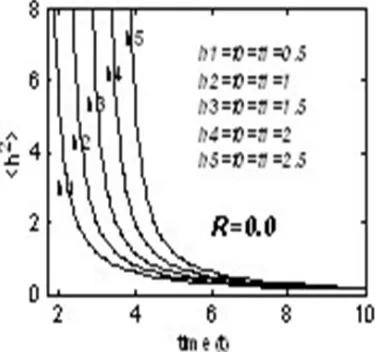
Fig. 4. Effects of energy decay curves of equation (36) for R=0.5.

(9)

Here h1, h2, h3, h4 and h5 are solutions of equation (36) in the chemical reaction at t₀=t₁ =0.5, 1, 1.5, 2, 2.5 corresponding with R =3, 2, 1, 0.5 and 0.0, which indicated in the Fig.1, Fig.2, Fig.3, Fig.4 and Fig.5 respectively. In the clean fluid h1, h2, h3, h4 and h5 are also solution curves of equation (37) which indicated in Fig.5.

.If the quadruple and quintuple correlations were not neglected, than more terms in negative higher power of

) t t

( − ₁ would be added to the equation (36), and for large times the last terms in the equations (36), becomes negligible, leaving the -3/2 power decay law for the final period in the first order chemical reaction. From Figure.1-5, we watch that energy decay curves successively increased for decreasing the values of M and maximum at the point where R is equal to zero. We conclude that the effect of first order reactant is most important that is in the present of chemical of magnetic field fluctuation the energy decay increases with the decreases of R and maximum for clean fluid that is for R=0.

Acknowledgements

Authors (M.A.Bkar Pk, Abdul Malek &M.A.K.Azad) are grateful to the Department of Applied Mathematics, University of Rajshahi, Bangladesh for giving all facilities and support to carry out this work.

References

[1] Azad M.A.K, Aziz M.A and Sarker M.S.A, “Statistical theory of certain distribution functions in MHD turbulent flow for velocity and concentration undergoing a first order reaction in a rotating system.” Bangladesh Journal of Scientific and Industrial Research, 46(1):59-68. 2011.

[2] Bkar Pk, M.A., M.A.K. Azad and M. S. Alam Sarker, “Decay of energy of MHD turbulence for four-point correlation.” International Journal of Engineering & Technology.1 (9):pp1-13. 2012.

[3] Bkar Pk. M.A., M. A. K. Azad and M. S. Alam Sarker, “First-order reactant in homogeneou turbulence prior to the ultimate phase of decay for four-point correlation in presence of dust particle,”Res.J.Appl.Sci.Eng. Technol.,5(2):585-595. 2013a.

[4] Bkar Pk, M.A., M.S.Alam Sarker and M.A.K. Azad, “Decay of MHD turbulence before the final period for four-point correlation in a rotating system.” Res. J. Appl. Sci. Eng. Technol., 6(15), 2789-2798. 2013b.

[5] Chandrasekhar, S., “The invariant theory of isotropic turbulence in magneto-hydrodynamics,” Proc. Roy. Soc., London, and A204:435-449. 1951.

[6] Corrsin, S., “On the spectrum of isotropic temperature fluctuations in isotropic turbulence.”J. Apll. Phys 22:469-473.1951.

[7] Deissler, R.G., “On the decay of homogeneous turbulence before the final period.” Phys.Fluid, 1:111-121. 1958. [8] Deissler, R.G., “A theory of decaying homogeneous

turbulence.” Phys. Fluid, 3:176-187. 1960.

[9] Islam, M.A. and M.S.A Sarker, “First order reactant in MHD turbulence before the final period of decay for the case of multi-point and multi-time.” Indian J. pure appl. Math., 32(8):1173-1184. 2001.

[10] Sarker, M. S. A. and N. Kishore, “Decay of MHD turbulence before the final period.” Int. J. Engng Sci., 29(11):1479-1485. 1991.

[11] Kumar, P. and S.R.Patel, “First-order reactant in homogeneous turbulence before the final period of decay.” Phys .Fluids, 17: 1362-1368. 1974.

[12] Kumar, P. and S.R.Patel, “First order reactant in homogeneous turbulence before the final period for the case of multi-point and multi-time.” Int. Eng. Sci, 13:305-315.1975.

[13] Hossain M. M, M. A. Bkar Pk and M.S. A. Sarker “Homogeneous fluid turbulence before the final period of decay for four-point correlation in a rotating system for first-order reactant.” American Journal of Theoretical and Applied Statistics, 3(4):81-89. 2014b.

[14] Bkar Pk, M.A., M. M. Hossain and M. A. K. Azad, “First-order reactant of homogeneous dusty fluid turbulence prior to the final period of decay in a rotating system for the case of multi-point and multi-time at four-point correlation.” Pure and Applied Mathematics Journal, 3(4):78-86.2014a.