Sufficient Dimensionality Reduction
Amir Globerson [email protected]
Naftali Tishby [email protected]
School of Computer Science and Engineering and The Interdisciplinary Center for Neural Computation The Hebrew University, Jerusalem 91904, Israel
Editors: Isabelle Guyon and Andr´e Elisseeff
Abstract
Dimensionality reduction of empirical co-occurrence data is a fundamental problem in unsuper-vised learning. It is also a well studied problem in statistics known as the analysis of cross-classified data. One principled approach to this problem is to represent the data in low dimension with min-imal loss of (mutual) information contained in the original data. In this paper we introduce an information theoretic nonlinear method for finding such a most informative dimension reduction. In contrast with previously introduced clustering based approaches, here we extract continuous
fea-ture functions directly from the co-occurrence matrix. In a sense, we automatically extract functions
of the variables that serve as approximate sufficient statistics for a sample of one variable about the other one. Our method is different from dimensionality reduction methods which are based on a specific, sometimes arbitrary, metric or embedding. Another interpretation of our method is as generalized - multi-dimensional - non-linear regression, where rather than fitting one regression function through two dimensional data, we extract d-regression functions whose expectation val-ues capture the information among the variables. It thus presents a new learning paradigm that unifies aspects from both supervised and unsupervised learning. The resulting dimension reduction can be described by two conjugate d-dimensional differential manifolds that are coupled through Maximum Entropy I-projections. The Riemannian metrics of these manifolds are determined by the observed expectation values of our extracted features. Following this geometric interpretation we present an iterative information projection algorithm for finding such features and prove its convergence. Our algorithm is similar to the method of “association analysis” in statistics, though the feature extraction context as well as the information theoretic and geometric interpretation are new. The algorithm is illustrated by various synthetic co-occurrence data. It is then demonstrated for text categorization and information retrieval and proves effective in selecting a small set of features, often improving performance over the original feature set.
Keywords: Feature Extraction, Maximum Entropy, Information Geometry, Mutual Information,
Association Analysis.
1. Introduction
A classic scenario in machine learning and statistics is that of identifying a source distribution from an i.i.d. sample generated by it. Given a sample xn= [x1,...,xn]generated i.i.d. by an unknown
distribution p(x|y), a basic task in statistical estimation is to infer the value of y from the sample. It is commonly assumed that the source distribution belongs to some parametric family p(x|y)where distributions’ “indices”, or “parameters” y∈Y may take an infinite set of values.1
A useful approach to this problem is to extract a small set of statistics or features, which are functions of the samples and use only their values for inferring the source parameters. Such statistics are said to be sufficient if they capture all the “relevant information” in the sample about the identity of y∈Y . As is well known, under certain regularity assumptions non-trivial sufficient statistics exist if and only if p(x|y)belongs to an exponential family (Pitman, 1936). Furthermore, the sufficient statistics can then be written as additive functions of the samples.
When p(x|y)does not belong to an exponential family there still exist statistics which capture
some of the information in the sample about the set Y . In this work we suggest a way of quantifying
this information using information theoretic notions and show how features which maximize this information can be extracted. Due to its link with the statistical concept of sufficiency, we call our method Sufficient Dimensionality Reduction (SDR).
An alternative view of this setup is a generalization of the problem of nonlinear regression. In regression problems, one assumes that the “relevant information” between two variables, X and Y , is captured by one unknown function, y= f(x)normally taken as the conditional expectation of x,
hxip(x|y), for each y∈Y . However, conditional expectations, which minimize the square-loss, may
not capture all the structure of the variables. There is often more information between X and Y than can be captured by a single conditional expectation value. Our problem then is to find several such functions, or regressors, that together capture more of the information and structure of the variables. As will be shown in this paper, this problem can be cast as finding dimension reduction which captures the mutual information in a two-way contingency table. It is thus related to a long line of work in statistics that started by Fisher (1940) with his canonical correlation decomposition, through the work of Haberman (1978) on Log-Linear models for frequency tables. Our formalism is most closely related to association models, developed by Goodman and others (see Goodman, 1985, for a thorough review). However, we link these ideas with feature extraction and machine learning and provide a novel information theoretic and geometric interpretations and algorithms for such analysis. Furthermore, our variational formulation of the problem enables further extensions to multivariate dimension reduction and discriminative feature extraction. Our work is also deeply related to a new information theoretic method for relevant clustering, the information bottleneck
method (Tishby et al., 1999), in which a discrete set of clusters that captures the mutual information
in a contingency table is generated. This method, in turn, is related to Rate-Distortion-Theory (lossy compression) on the one hand and to channel coding with letter cost on the other hand (see Cover and Thomas, 1991). Unlike these “classical” coding theorems, in the bottleneck method the relevant “distortion function”, or the “channel-cost” properties, are induced solely from the co-occurrence statistics.
Finally, our feature extraction problem turns out to be equivalent to a special matrix factorization problem, where a data joint distribution is approximated by an exponent of a low rank matrix. As such it is related to the rich literature on factorization of positive matrices (most recently to Lee and Seung, 1999, Hofmann, 2001). In this paper we describe an alternating projection algorithm for solving this special factorization problem, and compare its performance with other linear and non-linear methods. Our algorithm is based on repeated application of I-projections (Csiszar, 1975) where the roles of constraints and Lagrange multipliers are alternated repeatedly. Another feature learning algorithm that is based on a similar entropy Min-Max principle, but in a rather different setting, appeared recently in a paper by Zhu et al. (1997).
vari-able. By defining the information of the observations as the minimal mutual information among all joint distributions consistent with the observations, our problem can be formulated as a Max-Min Mutual-Information variational principle. We then show that this problem is equivalent to finding a model of a special exponential form which is closest to the empirical distribution (contingency ta-ble) in the KL-divergence (or Maximum Likelihood) sense. We next present an iterative algorithm for solving these problems and prove its convergence to a solution. An interesting information ge-ometric formulation of our algorithm is then suggested, which provides a covariant formulation of the extracted features. It also provides interesting sample complexity relations via the Cramer-Rao inequalities for the selected features. We conclude by demonstrating the performance of the algo-rithm, first on artificial data and then on a real-life document classification and retrieval problem.
2. Problem Formulation
To illustrate our motivation, consider a die with an unknown outcome distribution. Suppose we are given the mean outcome of a die roll. What information does it provide about the probability to obtain 6 in rolling this die? One possible “answer” to this question was suggested by Jaynes (1957) using his “Maximum Entropy (MaxEnt) principle”.
Denote by X ={1,...,6} the possible outcomes of the die roll, and by~φ(x) an observation, feature, or function of X . In the example of the expected outcome of the die, the observation is
~φ(x) =x, the specific outcome. Given the result of n rolls x1,...xn, the empirical expected value is ~a=1n∑ni=1~φ(xi). MaxEnt argues that the “most probable” outcome distribution ˜p(x)is the one with
maximum entropy among all distributions satisfying the observation constraint, D
~φ(x)
E
˜ p(x)=~a.
This distribution depends, of course, on the actual value of the observed expectation,~a.
The MaxEnt principle is considered problematic by many since it makes implicit assumptions about the distribution of the underlying “micro-states”, that are not always justified. In this example there is in fact a uniform assumption on all the possible sequences of die outcomes that are con-sistent with the observations. MaxEnt also does not tell us what are the features whose expected values provide the maximal information about the desired unknown - in this case the probability to obtain 6. This question is meaningful only given an additional random variable Y which denotes (parameterizes) a set of possible distributions p(x|y), and one measures feature quality with respect to this variable. In the die case we can consider the Y parameter as the probability to obtain 6. The optimal measurement, or observation, in this case is obviously the expected number of times 6 has occurred, namely, the expectation of the single featureφ(x) =δ(6−x). The interesting question is what is the general procedure for finding such features.
An important step towards formulating such a procedure is to define the information in a
mea-surement of a given feature vector~φ(x): X→ℜd, about the relevant variable Y . This information is also related to the question: how well can one predict the identity of Y from a sample of X generated by the source distribution p(x|y)?
To answer this, consider the set of all distributions ˜p(x,y)which agree with the given expecta-tions and margin distribuexpecta-tions, p(x)and p(y). The assumption that these marginals are known is not very limiting since they can be reliably estimated even from (relatively) small joint samples. This assumption also simplifies our analysis and algorithm considerably. Notice that the true distribu-tion is also in this set (up to possible finite sample errors in the expectadistribu-tions). For every distribudistribu-tion
˜
I[p˜(x,y)] =∑x,yp˜(x,y)logp˜p(˜x()xp,˜y()y)(Cover and Thomas, 1991).2 The measure of mutual information does not rely on any prediction process, but provides a bound on the error rate using any prediction scheme for the given distribution.
The information captured about Y precisely by the expected values of the measured features
~φ(x) can not be larger than the mutual information of any joint distribution consistent with these measurements - since all those distributions can produce these observations. It is thus natural to take the minimal possible value of I[p˜(x,y)], over the distributions consistent with the observations as the measure of the information (about Y) in the observations. Moreover, the distribution which minimizes this information has the largest possible prediction error of Y among all the distributions in this set. As we show later, this principle of minimum information coincides with finding the joint distribution with maximum entropy, subject to the observations and margin constraints, but without the hidden assumptions of the MaxEnt principle.
Formally, we define IM(~φ(x),p), the information in the measurement of~φ(x)on p(x,y)as:
IM(~φ(x),p)≡ min ˜
p(x,y)∈P(~φ(x)),p)
I[p˜(x,y)]. (1)
The set
P
(~φ(x),p)is the set of distributions that satisfy the constraints, defined byP
(~φ(x),p)≡n ˜
p(x,y): D
~φ(x)
E
˜ p(x|y)=
D
~φ(x)
E
p(x|y)
˜
p(x) =p(x)
˜
p(y) =p(y)
o
.
The desired most informative features~φ∗(x) are precisely those whose measurements provide the maximal information about Y . Namely,
~φ∗(x) =arg max ~φ(x)
IM(~φ(x),p).
Plugging in the definition of IMwe obtain the following Max-Min problem:
~φ∗(x) =arg max ~φ(x)
min
˜
p(x,y)∈P(~φ(x),p)
I[p˜(x,y)]. (2)
Notice that this variational principle does not define a generative statistical model and is in fact a model independent approach. As we show later, however, the resulting distribution ˜p(x,y), is necessarily of a special exponential form and can be interpreted as a generative model in that class. There is no need, however, to make any assumption about the validity of such a model for the empirical data. The data distribution p(x,y) is in fact needed only in order to estimate the
expectations D
~φ(x)
E
p(x|y)for every y (besides the marginals), given the candidate features
~φ(x). In practice these expectations are estimated from finite samples and empirical distributions. From a machine learning view our method thus requires only “statistical queries” on the underlying joint distribution (Kearns, 1993).
In the next section we show that the problem of finding the optimal functions~φ(x)is dual to the problem of extracting the optimal features for Y that capture information on the variable X , and in fact the two problems are solved simultaneously.
3. The Nature of the Solution
We first show that the problem as formulated in Equation 2 is equivalent to the problem of minimiz-ing the KL divergence between the empirical distribution p(x,y)and a special family of distributions of an exponential form. To simplify notation, we sometimes omit the suffix of(x,y)from the distri-butions. Thus ˜pt stands for ˜pt(x,y)and p for p(x,y)
Minimizing the mutual information in Equation 1 under the linear constraints on the expecta-tions
D
~φ(x)
E
p(x|y)is equivalent to maximizing the joint entropy:
H[p˜(x,y)] =−
∑
x,y
˜
p(x,y)log ˜p(x,y)
under these constraints, with the additional requirement that the marginals are not changed, ˜p(x) = p(x)and ˜p(y) =p(y). Due to the concavity of the entropy and the convexity of the linear constraints, there exists a unique maximum entropy distribution (for compact domains of x and y) which has the exponential form3(Cover and Thomas, 1991):
˜
p~∗φ(x)(x,y) = 1 Zexp
~φ(x)·~ψ(y) +A(x) +B(y) , (3)
where Z, the normalization (partition) function is given by:
Z≡
∑
x,yexp
~φ(x)·~ψ(y) +A(x) +B(y)
,
and the functions~ψ(y),A(x),B(y) are uniquely determined as Lagrange multipliers from the
ex-pectation values D
~φ(x)
E
p(x|y) and the marginal constraints. It is important to notice that while the
distribution in Equation 3 which maximizes the entropy is unique, there is freedom in the choice of the functions in the exponent. This freedom is however restricted to linear transformations of the vector-functions~ψ(y) and~φ(x) respectively, as long as the original variables X and Y remain the same, as we show later on.
The distributions of the form Equation 3 can also be viewed as a distribution class parametrized by the infinite family of functionsΘ= [~ψ(y),~φ(x),A(x),B(y)](note that we treatψandφ symmet-rically). We henceforth denote this class by PΘ.
The discussion above shows that for every candidate feature~φ(x), the minimum information in Equation 2 is the information in the distribution ˜p~∗φ
(x). As argued before, this is precisely the
information in the measurement of~φ(x)about the variable Y . We now define the set of information minimizing distributions
PΦ
⊂PΘ, as follows:PΦ
≡np˜∈PΘ:∃~φ(x): p˜=p˜~∗φ(x) o.
It can be easily shown that ˜p~∗φ
(x)is the only distribution in PΘsatisfying the constraints in
P
(~φ(x),p)(see: Della-Pietra et al. (1997)). Thus,
PΦ
can alternately be defined as:PΦ
=np˜∈PΘ:∃~φ(x): p˜∈P
(~φ(x),p)o
. (4)
Finding the optimal (most informative) features~φ∗(x)amounts now to finding the distribution in
PΦ
which maximizes the information:˜
p∗=arg max
˜ p∈PΦ
I[p˜].
The optimal~φ∗(x)will then be theφparameters of ˜p∗, as in Equation 2. For every ˜p∈
PΦ
one can easily show thatI[p˜] =I[p]−DKL[p|p˜], (5)
where DKL[p|q] =∑x,yp logpq is the Kullback-Liebler divergence between p and q. Equation 5
has two important consequences. First, it shows that maximizing I[p˜]for ˜p∈
PΦ
is equivalent to minimizing DKL[p|p˜]for ˜p∈PΦ
:˜
p∗=arg min
˜
p∈PΦDKL[p|p˜]. (6)
Second, Equation 5 shows that the information in I[p˜∗]cannot be larger than the information in the original data (the empirical distribution). This supports the intuition that the model ˜p∗ maintains only properties present in the original distribution that are captured by the selected features~φ∗(x).
A problem with Equation 6 is that it is a minimization over a subset of PΘ, namely
PΦ
. The following proposition shows that this is in fact equivalent to minimizing the same function over all of PΘ. Namely, the closest distribution to the data in PΘ satisfies the conditional expectation constraints and thus inPΦ
.Proposition 1
arg min
˜
p∈PΦDKL[p|p˜] =arg minp˜∈PΘDKL[p|p˜]
Proof: We need to show that the distribution which minimizes the right hand side is in
PΦ
. Indeed,by taking the (generally functional) derivative of DKL[p|p˜]w.r.t. the parametersΘin ˜p, one obtains
the following conditions:
∀y
D
~φ(x)
E
˜ p(x|y)=
D
~φ(x)
E
p(x|y) ∀x h~ψ(y)ip˜(y|x)=h~ψ(y)ip(y|x) ∀x p˜(x) =p(x) ∀y p˜(y) =p(y).
(7)
Clearly, this distribution satisfies the constraints in
P
(~φ(x),p)and from the definition in Equation 4 we conclude that it is inPΦ
.Our problem is thus equivalent to the minimization problem:
p∗=arg min
˜
p∈PΘDKL[p|p˜]. (8)
Notice that this minimization problem can be viewed as a Maximum Likelihood fit to the given
p(x,y) in the class PΘ, known as an association model in the statistical literature (see Goodman, 1985), though the context there is quite different. It is also interesting to write it as a matrix factor-ization problem (Matrix exponent here is element by element)
P= 1 Ze
ΦΨ (9)
where P is the distribution p(x,y), Φ is a |X| ×(d+2) matrix whose (d+1)th column is ones, and Ψ is a d+2× |Y| matrix whose (d+2)th row is ones (the vectors A(x),B(y) are the (d+
2)th column of Φ and (d+1)th row of Ψ). While the vectors A(x),B(y) are clearly related to the margin distributions p(x) and p(y), it is in general not possible to eliminate them and absorb them completely in the marginals. We therefore consider the more general form of PΘ. In the maximum-likelihood formulation of the problem, however, nothing guarantees the quality of this fit, nor justifies the class PΘ from first principles. We therefore prefer the information theoretic, model independent, interpretation of our approach. As will be shown, this interpretation provides us with powerful geometric structure and analogies as well.
4. An Iterative Projection Algorithm
The previous section showed the equivalence of the Max-Min problem, Equation 2 to the KL diver-gence minimization problem in Equation 8. We now present an iterative algorithm which provably converges to a local minimum of Equation 8, and hence solves the Max-Min problem as well. This minimization problem can be solved by a number of optimization tools, such as gradient descent or such iterative procedures as described by Goodman (1979). In what follows, we demonstrate some information geometric properties of this optimization procedure, thus constructing a general framework from which more general convergent algorithms can be generated.
The algorithm is described using the information geometric notion of I-projections (Csiszar, 1975). The I-projection of a distribution q(x)on a set of distributions
F
is defined as the distribution inF
which minimizes the KL-divergence DKL[p|q]. We denote this distribution by IPR(q,F):IPR(q,F)≡arg min
p∈FDKL[p|q].
An important property of the I-projection is the, so called, Pythagorean property (see e.g. Cover and Thomas, 1991, Ch. 12). If the set
F
is convex, then for every distribution p inF
, the following holds:DKL[p|q]≥DKL[p|IPR(q,
F
)] +DKL[IPR(q,F)|q].We now focus on the case where the set
F
is determined by expectation values. Given a d dimensional feature function~φ(x)and a distribution p(x), we consider the set of distributions which agree with p(x)on the expectation values of~φ(x), and denote it byF
(~φ(x),p(x)). Namely,F
(~φ(x),p(x))≡n ˜
p(x): D
~φ(x)E ˜ p(x)=
D
~φ(x)E p(x)
o
which is clearly convex due to the linearity of expectations. The I-projection in this case has the exponential form
IPR(q(x),F(~φ(x),p(x))) = 1
Z∗q(x)exp(~λ
Input:Joint (empirical) distribution p(x,y)
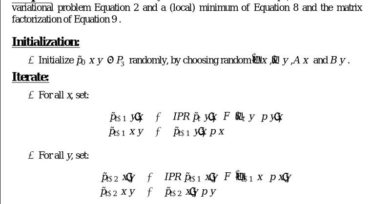
Output: 2d feature functions: ~ψ(y) and~φ(x) that result from ˜p∗, a solution of the variational problem Equation 2 and a (local) minimum of Equation 8 and the matrix factorization of Equation 9 .
Initialization:
• Initialize ˜p0(x,y)∈PΘrandomly, by choosing random~φ(x),~ψ(y),A(x)and B(y). Iterate:
• For all x, set:
˜
pt+1(y|x) = IPR(p˜t(y|x),F(~ψt(y),p(y|x))) ˜
pt+1(x,y) = p˜t+1(y|x)p(x).
• For all y, set:
˜
pt+2(x|y) = IPR(p˜t+1(x|y),F(~φt+1(x),p(x|y))) ˜
pt+2(x,y) = p˜t+2(x|y)p(y).
• Halt on convergence (when small enough change in ˜pt(x,y)is achieved).
Figure 1: The iterative projection algorithm.
where~λ∗ is a vector of Lagrange multipliers corresponding to the expectation D
~φ(x)
E
p(x)
con-straints. In addition, for this special exponential form, the Pythagorean inequality is tight and becomes an equality (Csiszar, 1975). This property is further linked to the notion of “geodesic lines” on the curved manifold of such distributions.
Before describing our algorithm, some additional notations are needed:
• p˜t(x,y)- the distribution after t iterations. • ~ψt(y)- the~ψ(y)functions for ˜pt(x,y). • ~φt+1(x)- the~φ(x)functions for ˜pt+1(x,y). • Θt - the full parameter set for ˜pt(x,y).
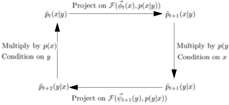
The iterative projection algorithm is outlined in Figure 1 and described graphically in Figure 2.
I-projections of (exponential) distributions are applied iteratively: Once for fixed~ψ(y) and their expectations, and then for fixed~φ(x)and their expectations. Interestingly, during the first projection, the functions~φ(x)are modified as Lagrange multipliers forh~ψ(y)ip˜(y|x), and vice-versa in the second projection. The iterations can thus be viewed as alternating mappings between the two sets of d-dimensional functions,~ψ(y)and~φ(x). This is also the direct goal of the variational problem.
We proceed to prove the convergence of the algorithm. We first show that every step reduces
DKL[p(x,y)|p˜t(x,y)].
Figure 2: The iterative projection algorithm: The dual roles of the projections that determine~ψ(y)
and~φ(x)as dual Lagrange multipliers in each iteration. These iterations always converge and the diagram becomes commutative.
1. ˜pt+1(y|x)is the I-projection of ˜pt(y|x)on the set
F
(~ψt(y),p(y|x)).2. p(y|x)is also in
F
(~ψt(y),p(y|x)).Using the Pythagorean property, (which is an equality here) we have:
DKL[p(y|x)|p˜t(y|x)] =DKL[p(y|x)|p˜t+1(y|x)] +DKL[p˜t+1(y|x)|p˜t(y|x)].
Multiplying by p(x)and summing over all x values, we obtain:
DKL[p|p˜t]−DKL[p(x)|p˜t(x)] =DKL[p|p˜t+1] +DKL[p˜t+1|p˜t]−DKL[p(x)|p˜t(x)].
where we used ˜pt+1(x) =p(x). Elimination of DKL[p(x)|p˜t(x)]from both sides gives:
DKL[p|p˜t] =DKL[p|p˜t+1] +DKL[p˜t+1|p˜t]. (10)
Using the non-negativity of DKL[p˜t+1|p˜t]the desired inequality is obtained: DKL[p|p˜t]≥DKL[p|p˜t+1].
Note that equality is obtained iff DKL[p˜t+1|p˜t] =0.
An analogous argument proves that:
DKL[p|p˜t+2]≤DKL[p|p˜t+1]. (11)
Proposition 3 If ˜pt =p˜t+2then the correspondingΘt satisfies ∂DKL[∂Θp|pΘ]Θ=Θt =0 .
In order to see that the algorithm indeed converges to a (generally local) minimum of DKL[p|pΘ],
note that DKL[p|p2t˜ ]is a monotonously decreasing bounded series, which therefore converges. Its
difference series (see Equation 10,11),
DKL[p|p˜t]−DKL[p|p˜t+2] =DKL[p˜t+1|p˜t] +DKL[p˜t+2|p˜t+1],
therefore converges to zero. Taking t to infinity, we get ˜pt+2= p˜t+1 =p˜t. Thus, the limit is a
stationary point of the iterations, and from proposition 3 it follows that it is indeed a local minimum of DKL[p|pΘ].4
4.1 Implementation - Partial I-projections
The description of the iterative algorithm assumes the existence of a module which calculates I-projections on linear (expectation) constraints. Because no general closed form solution for such a projection is available, it is found by successive iterations which asymptotically converge to the solution. It is rather straightforward to show that even if the projection algorithm uses only a ”Partial
I-projection” as its IPR module, it still converges to a minimum.
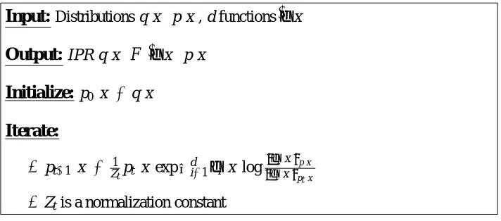
In this work, IPR was implemented using the Generalized Iterative Scaling (GIS) procedure (see Darroch and Ratcliff, 1972), described in Figure 3.
We now briefly address the computational complexity of our algorithm. The overall time com-plexity naturally depends on the number of iterations needed till convergence. In the experiments described in this work we ran the algorithm for up to 100 iterations, which produced satisfactory re-sults. The I-projection steps, which are performed using GIS, are iterative as well. We used 100-200 GIS iterations for each I−projection with a stopping condition when the ratio between empirical and model expectations was close enough to 1. Each step of the GIS has linear complexity in|X|d, where|X|is the size of the X variable and d the number of features. Since in each SDR iteration we perform I-projections for all X ’s and Y ’s, each iteration performs O(|X||Y||d|)operations.
The run-time of the algorithm is most influenced by the implementation of the I-projection algorithm. GIS is known to be slow to converge , but was used in this work for the simplicity of the presentation and implementation. Other methods that can speed this calculation by a factor of 20 have been suggested in the literature (Malouf, 2002) and should be used to handle large datasets and many features. This is expected to make SDR comparable to SVD based algorithms in computational complexity.
The parameters were always initialized randomly, but different initial conditions did not affect the results noticeably. Initializing the parameters using the SVD of the log of p(x,y) generated a better initial distribution but did not improve the final results, nor convergence time.
5. Information Geometric Interpretation
The iterative algorithm and the exponential form provide us with an elegant information geometric insight and interpretation of our method. The values of the variable X are mapped into the d-dimensional differential manifold described by~φ(x), while values of the variable Y are mapped into
4. In order to take this limit, we use the fact that ˜pt+1and ˜pt+2are continuous functions of ˜ptbecause the I projection
Input:Distributions q(x),p(x), d functions~φ(x)
Output:IPR(q(x),
F
(~φ(x),p(x)))Initialize:p0(x) =q(x) Iterate:
• pt+1(x) =Z1tpt(x)exp∑di=1φi(x)log h φi(x)ip(x)
hφi(x)ipt(x)
• Zt is a normalization constant
Figure 3: The Generalized Iterative Scaling Algorithm.
a d-dimensional manifold described by~ψ(y). Empirical samples of these variables are mapped into the same d-dimensional manifolds through the empirical expectations
D
~φ(x)
E
p(x|y)andh~ψ(y)ip(y|x)
respectively. These geometric embeddings, generated by the feature vectors Φand Ψ, are in fact curved Riemannian differential manifolds with conjugate local metrics (see Amari and Nagaoka, 2000).
The differential geometric structure of these manifolds is revealed through the normalization (partition) function of the exponential form, Z(φ;ψ). We note the following relations:
δlog Z
δφ = h~ψ(y)ip(y|x) (12)
δlog Z
δψ =
D
~φ(x)
E
p(x|y) (13)
and the second derivatives,
δ2log Z
δφiδφj =
(ψi(y)− hψi(y)i)(ψj(y)−
ψj(y)
)p(y|x) (14)
δ2log Z
δψiδψj =
(φi(x)− hφi(x)i)(φj(x)−
φj(x)
)p(x|y) . (15)
The last two matrices, which are positive definite, are also known as the Fisher information matrices for the two sets of parametersΦandΨ. Using the Information Geometry formalism of Amari, one can define the natural coordinates of those manifolds, as well as the geodesic projections, which are equivalent to the previously defined I-projections. The natural coordinates of the manifold are those that diagonalize the Fisher matrices locally, i.e. are locally uncorrelated. Moreover, the intrinsic geometric properties of these manifolds, such as their local curvature and geodesic distances are invariant with respect to transformations (including nonlinear) of the coordinates φand ψ. Since our iterative algorithm can be formulated through covariant projections, its fixed (convergence) point is also invariant to local coordinate transformations, as long as the above coupling between the two manifolds is preserved.
should be invariant to permutations of the rows and columns of the original co-occurrence matrix. This fact is illustrated in the next section. The information geometric formulation of the algorithm and its application to the study of geometric invariants requires further analysis.
5.1 Cramer-Rao Bounds and Uncertainty Relations
The special exponential form provides us with an interesting uncertainty relation between the con-jugate manifoldsΨandΦand a way to deal with finite sample effects.
For a general parametric family, p(x|θ), withθ the parameter vector, the Fisher information matrix,
Ji,j(θ) =
∂
log p(x|θ)
∂θi
∂log p(x|θ)
∂θj
x
=
−∂2log p∂θ (x|θ) i∂θj
x ,
provides bounds on the covariance matrix of any estimator of the parameter vector from a sample. Denoting such an estimator from an i.i.d. sample of size n, x(n), by ˆθ(xn), the covariance matrix of the estimators, Cov(θˆi,θˆj)is symmetric definite (if the parameters are linearly independent) and can
be diagonalized together with the Fisher information matrix. In particular, the diagonal elements of the two matrices satisfy the Cramer-Rao bound,
Ji,i(θ)Var(θˆi(xn))≥
1
n .
For our special exponential form this inequality yields a particularly nice uncertainty relation be-tween finite sample estimates of the feature vectors~φ(x) and~ψ(y), since for the exponential form the Fisher information matrices are dual as well,
Ji,j(ψ) = Cov(φˆ(xn))
Ji,j(φ) = Cov(ψˆ(xn))
and the Cramer-Rao inequalities, for the diagonal terms, become
Var(ψ)Var(φˆ(xn)) ≥ 1
n (16)
Var(φ)Var(ψˆ(xn)) ≥ 1
n (17)
as the Fisher information of theφfeature is just the variance of its adjointψvariable, and vice versa. In fact we know that this bound is tight precisely for exponential families, and Equations 16,17 are equalities.
These intriguing “uncertainty relations” between the conjugate features are strictly true only for the exponential form ˜p∗and hold only approximately for the true variances. Yet they provide a way to analyze finite sample fluctuations in the estimates of the features.
The information-geometric structure of the problem allows us to interpret our algorithm as alter-nating (geodesic) projections between the two Riemannian manifolds ofΨandΦ. These manifold allow an invariant formulation of the feature extraction problem through geometric quantities that do not depend on the choice of local coordinates, namely the specific choice of the functionsφ(x)
andψ(y). Among these invariants, the metric tensors of the manifolds provide us with the way to define and measure the geodesic projections. On the other hand, since these tensors are just the Fisher information matrices for the exponential forms, they provide us with bounds on the finite
6. Applications
The derivation of the SDR features suggests that they should be efficient in identifying a source distribution Y given a sample X1,...,Xnby using just the empirical expectations 1n∑in=1~φ(xi). We
next show how the SDR algorithm can extract non-trivial structure from both artificial data, and real-life problems.
6.1 Illustrative Problems
In this section, some simple scenarios are presented where regression, either linear or non-linear, does not extract the information between the variables. SDR is then shown to find the appropriate regressors and uncover underlying structures in the data.
The construction of the SDR features is based on the assumption that only the knowledge of the function~φ(x)and its expected values
D
~φ(x)
E
p(x|y) is required for estimating Y from X . Thus,
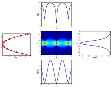
assuming the SDR approximation is valid, we can replace p(x,y) with the above two functions. However, it is clear that one can use the Lagrange multipliers~ψ(y)instead of the expected values, since there is a one to one correspondence between these two functions of Y . Finally, because the problem is symmetric w.r.t X and Y , we are also interested in the regressor averages h~ψ(y)ip(y|x), which together with~ψ(y)should provide optimal information about X . Figure 4 depicts these plots for running SDR with d=1 for the distribution:
p1(y|x)∼
N
(0,0.2+0.4|sin 2x|)where
N
(µ,σ) is a normal distribution with mean µ and standard deviation σ. This distribution is of an exponential form and has a single sufficient statistic: y2. The SDR single feature ψ(y)turns out to be nearly identical to y2, up to scaling and translation. The averageshψ(y)ip(y|x)and the corresponding φ(x) indeed reveal the periodic structure in the data, and are thus appropriate regressors for this problem.
In Figure 4, the numerical value of x,y was used for plotting the SDR features. However,
variables often cannot be assigned meaningful numerical values (e.g. terms in documents), and this approach cannot be used. One can still extract a description invariant representation in these cases by plotting the points~φ(x),~ψ(y)inℜd. This allows the analysis of the functional relation between the two statistics, without assuming any order on the x or y domains. To illustrate this, consider a scrambled version of the distribution:
p2(y|x) =
N
(2πsin x,0.8+0.1x)where both variables have undergone a random permutation. The scrambled distribution is shown in Figure 5, along with scatter plots of~ψ(y) and~φ(x). These plots illustrate the structure of the differential manifolds described in the previous section. Since both scatter plots are clearly one dimensional curves, the correct order of x and y was recovered by traversing the curves, and the resulting ”unscrambled distribution” is shown in Figure 5. It clearly demonstrates that the original continuous ordinal scale has been recovered.
Similar procedures can be used for recovering continuous structure from distributions with more than two statistics. Figure 6 shows the distribution:
p3(y|x) = 1 Zx
e−
(y−sin 2πx)2 2(0.8+0.1x)2−(
−2 −1 0 1 2 −2.5 −2 −1.5 −1 −0.5 φ (x) x
0 5 10 15 20
−2 −1.5 −1 −0.5 0 0.5 1 1.5 2 ψ(y) y x y
−2 −1 0 1 2
−2 −1.5 −1 −0.5 0 0.5 1 1.5 2
−1 −0.9 −0.8 −0.7 −0.6 −2 −1.5 −1 −0.5 0 0.5 1 1.5 2
<φ(x)>
y
−2 −1 0 1 2
−1 −0.5 0 0.5 1 < ψ (y)> x
Figure 4: SDR feature extracted for the distribution p1(y|x)∼
N
(0,0.2+0.4|sin 2x|). Middle: Thedistribution p1. Left: The SDR feature for y: ~ψ(y)in blue, and a scaled and translated y2 in red dots. Bottom: Expected valueh~ψ(y)ip(y|x) as a function of x. Top: The SDR feature for x:~φ(x). Right: Expected value
D
~φ(x)
E
p(x|y)as a function of y.
x
y φ(x)2
φ1(x)
ψ2
(y)
ψ1(y) x
y
Figure 5: Reordering X and Y using SDR. From left to right: 1: The scrambled version of p2(y|x) =
N
(2πsin x,0.8+0.1x)2: Scatter plot of φ2(x)vs. φ1(x)- the~φ(x) curved manifold. 3:This distribution has four sufficient statistics, namely y,y2,y3,y4. However, SDR can still be used with d=2 to represent both X and Y as two dimensional curves, as shown in Figure 6. Although two statistics do not capture all the information in the distribution, the two curves still reveal the underlying parameterization. Specifically, the original order in the X and Y domains can be recon-structed.
x
y φ(x)2
φ1(x)
ψ2
(y)
ψ1(y)
Figure 6: SDR analysis of p3(x,y). Left The distribution p3(x,y). Middle: Scatter plot for the
manifold~φ(x). Right: Scatter plot for the manifold~ψ(y).
6.2 Document Classification and Retrieval
The analysis of large databases of documents presents a challenge for machine learning and has been addressed by many different methods (see Yang and Liu, 1999, for a recent review). Important applications in this domain include text categorization, information retrieval and document cluster-ing.
Several works use a probabilistic and information theoretic framework for this analysis (Hof-mann, 2001, Slonim and Tishby, 2000), whereby documents and terms are considered stochastic variables. The probability of a term w∈ {w1,...,w|W|}appearing in a document doc∈ {doc1,...,doc|doc|}
is denoted p(w|doc)and is obtained from the normalized term count vector for this document:
p(w|doc) = n(doc,w)
∑wn(doc,w) ,
where n(doc,w) is the number of occurrences of term w in document doc. The joint distribution
p(w,doc) is then calculated by multiplying by a document prior p(doc) (e.g. uniform or propor-tional to document size). This stochastic relationship is then analyzed using an assumed underlying generative model, e.g. a linear mixture model as in the paper of Hofmann (2001), or a maximum entropy model as in the paper of Nigam et al. (1999). An optimal model is found, and used for predicting properties of unseen documents.
In the current work, SDR is used for finding term features~φ(w) such that using their mean values alone we can infer information about document identity. This approach is nonlinear and thus significantly differs from linear based approaches such as LSI (Deerwester et al., 1990) or PLSI (Hofmann, 2001).
50 100 150 200 250 0.2
0.4 0.6 0.8 1 1.2 1.4 1.6
KL(p;p
*)
d
50 100 150 200 250 0.5
1 1.5 2 2.5 3 3.5
I(p
*)
d
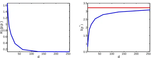
Figure 7: Left: KL between the original distribution and the model, for different d values. Right: Information in the model. The horizontal line marks the information in the original dis-tribution.
space (e.g. positivity, range etc.) and performs a completely unsupervised search for the optimal
~φ(w).
6.2.1 DOCUMENTINDEXING USINGSDR
The output of the SDR algorithm can be used to represent every document by an index in ℜd. This transformation reduces the representation of a document from|W|, the number of terms in the corpus, to d dimensions. Such a dimensionality reduction serves two purposes: First, to extract relevant information and eliminate noise. Second, low dimensional vectors can allow faster, more efficient information retrieval, an important feature in real world applications. The resulting indices can be used for document retrieval or categorization.
A natural index is the expected value of~φ(w)for the given document: ˆφ(doc)≡
D
~φ(w)
E
p(w|doc).
Since the SDR formulation assumes only knowledge of expected values can be used, it is sensible to represent a document using this set of values. Alternatively, one can use the set of Lagrange multipliers ~ψ(doc) for each document in the training data. Given a new document, not in the training data, one can find~ψ(doc)using a single I-projection of p(w|doc)on the linear constraints imposed by~φ(w).
6.2.2 DOCUMENTCLASSIFICATION APPLICATION
We used the 20Newsgroups database (Lang, 1995) to test how SDR can generate small features sets for document classification.
We start with an illustrative example, which shows how SDR features capture information about document content. We chose two different newsgroups with subjects : ”alt.atheism” and ”comp.graphics”, and preselected 500 terms and 500 documents per subject, using the informa-tion gain criterion (Yang and Liu, 1999). The projecinforma-tion algorithm was then run on the resulting
p(w,doc)matrix, for values of d=1,2,4,8,... ,256. Figure 7 shows DKL[p|p∗], I[p∗]as a function
of d. It can be seen that as larger values of d are used, the original distribution is approached in the KL sense and in the mutual information sense (as in Equation 5).
−200 −10 0 10 20 0.1
0.2 0.3 0.4 0.5
Val
p(Val)
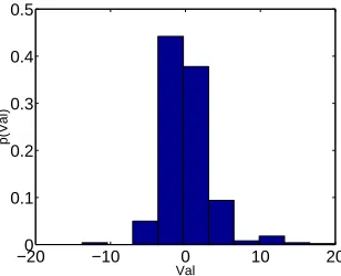
Figure 8: Histogram of~φ(w)values.
fatwa rushdie islam muslims islamic
correction gamma jfif fullcolor lossless
Figure 9: Terms with high (right) and low (left)φ1(w)values
the terms with high~φ(w)correspond to the ”comp.graphics” subject, and the ones with low~φ(w)
correspond to ”alt.atheism”. This single feature thus maps the terms into a continuous scale through which it assigns positive weights to one class, negative weights to the other, and negligible weights to terms which are possibly irrelevant to the classes.
We next performed classification on eight different pairs of newsgroups. The ˆφ(doc) index was used as input to a support vector machine (SVM-Light Joachims, 1998), which was trained to classify documents according to their subjects. Baseline results were obtained by running the SVM classifier on the original p(w|doc) vectors. The training and testing sets consisted of 500 documents per subject, and 500 terms. We experimented with values d =1,2,4,8,... ,256,500 to test how well we can classify with relatively few features. Figure 10 shows the fraction of the baseline performance that can be achieved using a given number of features. It can be seen that even when using only four features, 98% of the baseline performance can be achieved.
Thus, classification based on the SDR index achieves performance comparable to that of the baseline, even though it uses significantly less features (compared to the 500 features used by the baseline classifier). Importantly, the features were obtained in a wholly unsupervised manner, and have still discovered the document properties relevant for classification.
6.2.3 INFORMATIONRETRIEVAL APPLICATION
Automated information retrieval is commonly done by converting both documents and queries into a vector representation, and then measuring their similarity using the cosine of the angle between these vectors (Deerwester et al., 1990).
SDR offers a natural procedure for converting documents into d dimensional indices, namely ˆ
100 101 102 0.92
0.94 0.96 0.98 1
SDR/Baseline Accuracy
Figure 10: Fraction of baseline performance achieved by using a given number of SDR features. Results are averaged over eight newsgroup pairs.
The following databases were used to test information retrieval: MED(1033 documents, 5381 terms), CRAN (1400 documents, 4612 terms) and CISI (1460 documents, 5609 terms).5 For each database, precision was calculated as a function of recall at levels 0.1,0.2,... ,0.9. The performance was then summarized as the mean precision over these 9 recall levels (see Hofmann, 2001).
We compared the performance of the SDR based indices with that of indices generated using the following algorithms:
• RAW-TF: Uses the original normalized term count vector p(w|doc)as an index. The dimen-sion of the index is the number of terms.
• Latent Semantic Indexing (LSI): LSI is, like SDR, a dimensionality reduction mechanism, which uses the Singular Value Decomposition (SVD) to obtain a low rank approximation of the term-frequency matrix: p(doc,w)≈U SV , where U is a|doc|×d matrix , S is d×d and V
is d× |w|. A new document vector~x is then represented by the d dimensional vector S−1V~x. • Log LSI: Since SDR is related to performing a low rank approximation of the log of p(w,doc),
we also tried to perform LSI where the input matrix is log p(w,doc). In order to avoid taking a log of zero, we thresholded the matrix to 10−7.
• Locally Linear Embedding (LLE) (Roweis and Saul, 2000): LLE performs a non linear ap-proximation of the manifold on which the vectors p(w|doc) lie. It maps these vectors into a d dimensional space, while preserving the neighborhood structure in the original, high-dimensional, space. LLE has been shown to perform well for image, as well as document data. For the experiments described here, we followed the procedure used by Roweis and Saul (2000),6 using the dot product between document vectors as the neighborhood metric, and taking 10 nearest neighbors (other values were experimented with, but 10 gave optimal performance). The version of LLE used here cannot index new vectors (although such an
5. The list of terms used can be obtained from www.cs.utk.edu/∼lsi/corpora.html
20 40 60 80 100 120 0.25
0.3 0.35 0.4 0.45 0.5 0.55
20 40 60 80 100 120
0.15 0.2 0.25 0.3 0.35 0.4
20 40 60 80 100 120
0.08 0.1 0.12 0.14 0.16 0.18
Figure 11: Mean precision as a function of index dimension for four indexing algorithms (SDR in circles, LSI in triangles, LogLSI in diamonds and LLE in squares), and three databases (from left to right: MED,CRAN,CISI). Horizontal line is the mean precision of the RAW-TF algorithm.
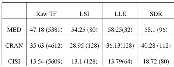
Raw TF LSI LLE SDR
MED 47.18 (5381) 54.25 (80) 58.25(32) 58.1 (96)
CRAN 35.63 (4612) 28.95 (128) 36.13(128) 40.28 (112)
CISI 13.54 (5609) 13.1 (128) 13.79(64) 18.72 (80)
Table 1: Mean precision results for information retrieval for several databases and different index-ing algorithms. Numbers in brackets are the number of features for which the optimal performance is obtained
extension was given by Roweis et al., 2001), so document and query data were indexed si-multaneously. Note that this gives LLE an advantage over the other indexing algorithms, since the test data (i.e. the queries) is used in the training procedure.
For each of the databases, indexing dimensions of d=8,16,32,48,... ,128 were used. Figure 11 shows the mean precision as a function of index dimension for the four indexing algorithms. Table 1 gives the peak performance on each of the databases for each of the algorithms (LogLSI is not in-cluded since it was inferior to LSI). It can be seen that SDR performs uniformly better than the other algorithms for most index sizes. Moreover, SDR achieves high performance for a small number of features, where other methods perform poorly. This suggests that SDR succeeds at capturing the low dimensional manifold on which the documents reside. The fact that LogLSI performs poorly shows that SDR is not equivalent to an SVD low rank approximation of log p(w,doc).
7. Discussion
inferring an unknown “variable” or other “relevant property” of the statistical data. The main goal of this procedure is to reveal possible continuous low-dimensional underlying structure that can “explain” the dependencies among the variables. Yet our applications suggest that the extracted continuous features can be used successfully for prediction of the relevant variable. An interesting question is in what sense is this resulting prediction close to optimal? In other words, how well can one infer using the extracted features compared the optimal inference procedure? The prediction error of an optimal procedure is the Bayes error (Devroye et al., 1996). When the true underlying distribution is of an exponential form with the correct dimensionality SDR is equivalent to max-imum likelihood estimation of its parameters/features, and as such is consistent (Devroye et al., 1996) and achieves asymptotically the optimal error in this case.
In the more interesting case, where the source distribution is not in the special exponential form, SDR should be interpreted as an induction principle, similar - but better motivated - than the maximum entropy principle. In fact it solves an inverse problem to that of MaxEnt, by finding the
optimal set of constraints - or observables - that capture the mutual information in the empirical
joint distribution. It is obvious that methods that exploit prior knowledge about the true distribution can do better in such cases. However, assuming that only empirical conditional expectations of given single variable functions are known about the source joint distribution (similar to “statistical queries” in machine learning, see Kearns, 1993) our Max-Min mutual information principle is a most reasonable induction method.
We briefly address several other important issues that our procedure raises.
7.1 Information in Individual Features
The low rank decomposition calculated using SVD suggests a clear ordering on the features using their associated singular values. Moreover, the SVD solutions are nested (i.e. the optimal features for d=2 are a subset of those for d=3). Due to its non-linear nature, the SDR solution is not necessarily nested (this is also true for solutions of linear based methods like those in Hofmann, 2001, Lee and Seung, 1999).
However, given a set of optimal SDR features~φ∗(x), the information in a single feature can be quantified in several ways. The simplest measure is IM(φ∗i(x)) (as defined in Equation 1), which
reflects the information obtained when measuring only φ∗i(x). Another measure is IM(~φ∗(x))− IM(φ∗1(x),...,φ∗i−1(x),φ∗i+1(x),φ∗d(x)) which is the information lost as a result of not measuring
φ∗
i(x). The two measures reflect different properties of the feature, and further research is required to
test their usefulness, for example in assigning confidence to the measurement of different features.
7.2 Finite Samples
The basic assumption behind our problem formulation is that we have access to the true expectation values h~ψ(y)i and h~φ(x)i. These can be estimated uniformly well from a finite sample under the standard uniform convergence conditions. In other words, standard learning theoretical techniques can give us the sample complexity bounds, given the dimensions of X and Y and the reduced di-mension d. For continuous X and Y further assumptions must be made, such as the fat-shattering dimension of the features.
the finite sample effects, as we discussed in section 5.1. We can then bound the prediction errors in terms of the empirical covariance matrices of the obtained features.
7.3 Uniqueness of the Solution
The optimal features are not unique in the following sense: since only the dot-product~φ(x)·~ψ(y)
appears in the distribution ˜p(x,y), any invertible matrix R can be applied such that~φ(x)R−1 and
R~ψ(y)are equivalent to~φ(x) and~ψ(y). Note, however, that although the resulting functions~ψ(y)
and~φ(x)may depend on the initial point of the iterations, the information extracted does not (for the same optimum).
One can remove this ambiguity by orthogonalization and scaling of the feature functions, for ex-ample by applying Singular Value Decomposition (SVD) to log ˜p(x,y)(see Becker and Clogg, 1989, for additional normalization schemes). Another is to de-correlate the~φ(x)using an appropriate lin-ear transformation. Notice, however, that our procedure is very different from direct application of SVD to log p(x,y). These two coincide only when the original joint distribution is already of the exponential form of Equation 3. In all other cases SVD based approximations (LSI included) will not preserve information as well as our features at the same dimension reduction.
7.4 Information Theoretic Interpretation
Our information MaxMin principle is close in its formal structure to the problem of channel capacity with some channel uncertainty (see e.g. Lapidoth and Narayan, 1998). This suggests the interesting interpretation for the features as channel characteristics. If the channel only enables the reliable transmission of d expected values, then our~ψ(y) exploit this channel in an optimal way. The channel decoder of this case is provided by the vector~φ(x)and the decoding is performed through a dot-product of these two vectors. This intriguing interpretation of our algorithm obviously requires further analysis.
7.5 Relations to Other Methods
Dimension reduction and clustering algorithms have become a fundamental component in unsu-pervised large scale data analysis. SDR is a dimension reduction method in that it reduces the description of the distribution p(x,y)from|X||Y|components to(d+1)(|X|+|Y|). There is a large family of algorithms with a similar purpose, which are based on a linear factorization of p(x,y). For example Hofmann (2001) and Lee and Seung (1999) suggest finding positive matrices Q of size
|X| ×d and R of size d× |Y|such that p=QR. Their procedure relies on the fact that the rows (or
columns) of p lie on a d dimensional plane. The SVD based LSI method (Deerwester et al., 1990) also performs a linear factorization of p, but it is not required to be positive.
Our approach is equivalent to approximating p (in the KL-divergence sense) by Z1eQR where
Q and R are matrices of size|X| ×(d+2)and (d+2)× |Y|respectively. Since the exponent can
An information theoretic approach to feature selection is also used by Zhu et al. (1997), in the context of texture modeling in vision. Their approach is similar to ours in that they arrive at a min-max entropy formulation. However, in contradistinction with the current work, they assume a specific underlying parametric model, and also define a finite feature set from which features are chosen using a greedy procedure. In this sense, their algorithm is more similar to the feature selection mechanism of Della-Pietra et al. (1997). There are also several works which search for approximate sufficient statistics (see Wolf and George, 2000, Geiger et al., 1998) by directly calcu-lating the information between the statistic and the parameter of interest. This results in a formalism different from ours, and usually necessitates some modeling assumptions to make computation fea-sible.
Since SDR finds a mapping from the X and Y variables into d dimensional space, it can be considered an embedding algorithm. As such, it is related to non-linear embedding algorithms, notably multi-dimensional scaling (Cox and Cox, 1994), Locally Linear Embedding (Roweis and Saul, 2000) and IsoMAP (Tenenbaum et al., 2000). Such algorithms try to preserve properties of points in high dimensional space (e.g. distance, neighborhood structure) in the embedded space. SDR is not formulated in such a way, but rather requires that the original points can be reconstructed optimally from the embedded points, where the quality of reconstruction is measured using the KL-divergence.
7.5.1 RELATIONS TO THEINFORMATIONBOTTLENECK
A closely related idea is the Information Bottleneck (IB) Method (originated in Tishby et al., 1999) which aims at a clustering of the rows of p(x,y)that preserves information. In a well defined sense, the IB method can be considered as a special case of SDR, when the features functions are restricted to a finite set of values that correspond to the clusters. However, clustering may not be the correct answer for many problems where the relationship between the variables comes from some hidden low dimensional continuous structures. In such cases clustering tends to quantize the data in a rather arbitrary way, while low dimensional features are simpler and easier for interpretation.
On the other hand, the motivation behind SDR is essentially the same as that of the IB, to find low-dimensional/complexity representations of one variable that preserve the mutual information about another variable. The algorithm in that case is however quite different and it solves in fact a more symmetric problem - find low dimensional representations of both variables (X and Y ) such that the mutual information between them is captured as good as possible. This is closely related to the symmetric version of the information bottleneck that is discussed by Friedman et al. (2001). As in the IB, the quality of the procedure can be described in terms of the “information curve” - the fraction of the mutual information that can be captured as a function of the reduced dimension. An interesting open question, at this point, is if we can extend the SDR algorithm to deal with different dimensions simultaneously. One would like to move continuously through more and more complex representations, as done in the IB through a mutual information constraint on the complexity of the representation. There are good reasons to believe that such an extension, that may “soften” the notion of the dimension, is possible also with SDR.
8. Conclusions and Further Research
nonlinear, and aims directly at preserving mutual information in a given empirical co-occurrence matrix. This is achieved through an information variation principle that enables us to calculate simultaneously informative feature functions for both random variables. In addition we obtain an exponential model approximation to the given data which has precisely these features as dual sets of sufficient statistics. We described an alternating projection algorithm for finding these features and proved its convergence to a (local) optimum. This is in fact an algorithm for extracting optimal sets of constraints from statistical data.
Our experimental results show that our method performs well on language related tasks, and does better than other linear models, which have been used extensively in the past. Performance is enhanced both in using smaller feature sets, and in obtaining better accuracy. Initial experiments on image data also show promising results. Taken together, these results suggest that the underly-ing structure of non-negative data may often be captured better by SDR than usunderly-ing linear mixture models.
One immediate extension of our work is to the multivariate case. The natural measure of infor-mation in this case is the multi-inforinfor-mation (see Friedman et al., 2001). One can then generalize the bivariate SDR optimization principle, thus defining an optimal measurement on a large set of variables.
Acknowledgments
We thank Noam Slonim, Gal Chechik and Amir Navot for helpful discussions and comments and for help with the experimental data. This research was supported by grants from the Israeli Academy of Science and from the Ministry of Science. A.G. is supported by the Eshkol Foundation.
References
S. Amari and N. Nagaoka. Methods of Information Geometry. Oxford University Press, 2000.
M.P. Becker and C.C. Clogg. Analysis of sets of two-way contingency tables using association models. Journal of the American Statistical Association, 84(405):142–151, 1989.
A.L. Berger, S.A. Della-Pietra, and V.J. Della-Pietra. A maximum entropy approach to natural language processing. Computational Linguistics, 22(1):39–71, 1996.
T.M. Cover and J.A Thomas. Elements of information theory. Wiley, 1991.
T. Cox and M. Cox. Multidimensional Scaling. Chapman and Hall, 1994.
I. Csiszar. I-divergence geometry of probability distributions and minimization problems. Annals
of Probability, 3(1):146–158, 1975.
J.N. Darroch and D. Ratcliff. Generalized iterative scaling for log-linear models. Ann. Math. Statist., 43:1470–1480, 1972.