A Generalized Kernel Approach to Dissimilarity-based Classification

A Generalized Kernel Approach to Dissimilarity-based

Classification

El ˙zbieta Pekalska [email protected]

Pavel Pacl´ık [email protected]

Robert P.W. Duin [email protected]

Pattern Recognition Group, Faculty of Applied Sciences Delft University of Technology

Lorentzweg 1, 2628 CJ Delft, The Netherlands

Editor:Nello Cristianini, John Shawe-Taylor and Robert Williamson

Abstract

Usually, objects to be classified are represented by features.In this paper, we discuss an alternative object representation based on dissimilarity values.If such distances separate the classes well, the nearest neighbor method offers a good solution.However, dissimilarities used in practice are usually far from ideal and the performance of the nearest neighbor rule suffers from its sensitivity to noisy examples.We show that other, more global classification techniques are preferable to the nearest neighbor rule, in such cases.

For classification purposes, two different ways of using generalized dissimilarity kernels are considered.In the first one, distances are isometrically embedded in a pseudo-Euclidean space and the classification task is performed there.In the second approach, classifiers are built directly on distance kernels.Both approaches are described theoretically and then compared using experiments with different dissimilarity measures and datasets including degraded data simulating the problem of missing values.

Keywords: dissimilarity, embedding, pseudo-Euclidean space, nearest mean classifier, support vector classifier, Fisher linear discriminant

1. Introduction

Since a lot of attention has been paid to similarity kernels, this paper is devoted to classification aspects using dissimilarity (or distance) kernels.Here, we want to emphasize the importance of recognition tasks for which dissimilarity kernels are built directly on images or shapes.Therefore, no feature space is (or needs to be) originally defined, but dissimilarities arise directly from the application.Examples are Jain and Zongker (1997) and Jacobs et al.(2000). Therefore, concerning the notation, if we generally refer to objects, like r, s orx, they will not be printed in bold, to emphasize that they are not (or might not) be feature vectors.The distance kernel represents the information in a relative way, i.e. through pairwise dissimilarity relations between objects.The goal now is to learnonly from such relational data, i.e. without any use (different than computing distances if necessary) of a starting original representation.The question studied here is, therefore, how to learn from data, given only dissimilarity kernels.

Recently, Sch¨olkopf (2000) has proposed to treat kernels as generalized distance mea-sures and also strengthened the link to algorithms based on positive definite kernels, such as the support vector classifier (SVC) (Vapnik, 1995, Sch¨olkopf, 1997) or the kernel prin-cipal component analysis (Sch¨olkopf et al., 1999, Sch¨olkopf, 1997).There is, however, an essential difference with our approach.Sch¨olkopf starts his reasoning from a feature space representation, where, in our case, this is not possible; we start a learning task from a dissimilarity kernel.For a more elaborate discussion, see Section 4.4.

Our principal question is how, given a dissimilarity kernel, a recognition problem can be tackled.To this end, we collected a set of methods which can be used by a researcher.In the paper we analyze the problem and illustrate possible solutions.Given a good dissimilarity measure, thek-nearest neighbor (k-NN) classifier is expected to perform well.It is, however, difficult to build such a measure for a complex recognition problem.In case of imperfect dissimilarities, thek-NN rule suffers from its sensitivity to noisy examples, but more global classifiers can perform better.How to design them is the goal of this research.

Two distinct approaches for classification tasks are studied in this paper.In the first one, a dissimilarity representation is isometrically embedded in a feature space, as presented in Section 3.This is always possible for a finite representation, although such a space may be pseudo-Euclidean (Goldfarb, 1985).Objects mapped to such a space preserve the structure of the data revealed in original distances.It means that if the dissimilarity measure defines classes which are bounded and compact, the configuration found in an underlying feature space should reflect those properties.An underlying feature space is constructed in the process of embedding.For this purpose, both the compactness hypothesis and its reverse should hold (see Section 2).If the dimensionality of such a feature space is low, then a classification task can be easily performed.

In the second approach, a dissimilarity kernel is interpreted as a mapping based on a chosen representation setRof objects (Duin, 2000, Pekalska and Duin, 2001), as presented in Section 5.In this formulation, classifiers can be constructed directly on the dissimilarity kernels, as in dissimilarity spaces.

dissimilarity kernels.Sections 6 and 7 describe the experiments conducted, and discuss the results.Conclusions are summarized in Section 8.

2. On dissimilarity measures

In general, a classification problem can be solved based on the so-called compactness hy-pothesis (Arkadev and Braverman, 1966, Duin, 1999), which states that objects that are similar, are also close in their representations.Effectively, this puts a constraint on the dissimilarity measure d, which has to be such that d(r, s) is small if objects r and s are similar, i.e. it should be much smaller for similar objects than for objects that are very different.For feature representations, the above does not hold the other way around: two entirely different objects may have the same feature representation.This does not cause a problem if these feature values are improbable for all or for all but one of the classes.For a dissimilarity kernel, however, the reverse of the compactness hypothesis also holds provided that the dissimilarity measure d poses some continuity.If we demand that d(r, s) = 0, if and only if objects r and s are identical, this implies that they belong to the same class. This can be extended somewhat by assuming that all objectsswith a small distance to the object r, i.e. for which d(r, s) < for a positive being sufficiently small, are so similar tor, that they belong to the same class.Consequently, the dissimilarities ofr ands to all objectsxunder consideration should be about the same, i.e. d(r, x)≈d(s, x).We conclude, therefore, that for dissimilarity representations satisfying the above continuity, the reverse of the compactness hypothesis holds: objects that are similar in their representation are also similar in reality and belong, thereby, to the same class (see Duin and Pekalska, 2001). As a result, classes do not overlap and the classification error may become zero for large training sets.

In order to interpret further such a hypothesis, let us recall the notion of metric.A dis-tance measuredis called a metric when the following conditions are fulfilled:

• reflectivity, i.e. d(x, x) = 0

• positivity, i.e. d(x, y)>0 if x is distinct fromy

• symmetry, i.e. d(x, y) =d(y, x)

• triangle inequality, i.e. d(x, y)< d(x, z) +d(z, y) for everyz

3. Linear embedding of dissimilarities

There is a number of ways to embed dissimilarity data in a feature space.Since, we are interested in a faithful configuration, a (non-)linear embedding is performed such that the distances are preserved as well as possible.Since nonlinear projections require more compu-tational effort and, moreover, the way of projecting new points to the existing configuration is not straightforward (or not defined), the linear mappings are preferable.Here, isometric embeddings are considered.

3.1 Embedding of Euclidean distances

Let the representation set R = {p1, p2, . . . , pn} refer to n objects (Duin, 2000, Pekalska

and Duin, 2001).Given an Euclidean distance matrix D∈ Rn×n between those objects, a distance preserving mapping onto an Euclidean space can be found.Such a projection is known in the literature as a classical scaling or a metric multidimensional scaling (Young and Householder, 1938, Borg and Groenen, 1997, Cox and Cox, 1995).In other words, the dimensionalityk≤nand the configurationX ∈ Rn×kcan be found such that the (squared) Euclidean distances are preserved.Note that having determined one configuration, another one can be found by a rotation or a translation.To remove the last degree of freedom, without loss of generality, the mapping will be constructed such that the origin coincides with the centroid (i.e. the mean vector) of the configuration X.1

To define X, the relation between Euclidean distances and inner products are used. First, it can be proven that

D(2)=b1T +1bT −2B,

(see Borg and Groenen, 1997, Appendix A.2), where D(2) is a matrix of square Euclidean distances, B is the matrix of inner products of the underlying configuration X, i.e. B = X XT and bis a vector of the diagonal elements ofB. B can also be expressed as:

B=−1 2J D

(2)_{J, (1)}

where J is the centering matrix J = I − 1_n1 1T _{∈ R}n×n _{and I is the identity matrix. J}

projects2the data such that the final configuration has zero mean. Bis positive definite since it is a Gram matrix (Greub, 1975).Then, the factorization of B by its eigendecomposition can be found as:

X XT =B =QΛQT, (2)

where Λ is a diagonal matrix with the diagonal consisting of the first non-negative eigen-values, ranked in descending order, followed by the zero eigen-values, and Q is an orthogonal matrix of the corresponding eigenvectors (Borg and Groenen, 1997).For k ≤ n non-zero eigenvalues, a k-dimensional representationX can be then found as:

X=QkΛ 1 2

k, Qk∈ R

n×k_{, Λ}12 k ∈ R

k×k_{, (3)}

1. It is also possible that any arbitrary point ofX would become the centroid.

2. A more general projection can be achieved, imposing that a weighted mean becomes zero, by which

where Qk is a matrix of the firstk leading eigenvectors and Λ 1 2

k contains the square roots

of the corresponding eigenvalues.Note that X, determined in this procedure, is unique up to rotation (the centroid is now fixed), since for any orthogonal matrix T, X XT ₌

(XT) (XT)T.Note also, that features ofXare uncorrelated, since the estimated covariance matrix of X becomes:

Cov(X) = 1 n−1X

T _X= 1

n−1Λ

1 2 k Q

T kQkΛ

1 2 k =

1

n−1Λk, (4)

because Qk is orthogonal.

3.2 Embedding of non-Euclidean distances

The matrixB=−1₂J D(2)J is positive definite if and only if the distance matrixD∈ Rn×n is Euclidean (Borg and Groenen, 1997, Gower, 1986, 1982).Therefore, for a non-Euclidean D, B is not positive definite, i.e. B has negative eigenvalues.As a result, X cannot be constructed fromB, since it relies on the square roots of eigenvalues; see Formula (3).Two approaches are possible to address this problem in an Euclidean space:

• Only p positive eigenvalues are taken into account, resulting in ap-dimensional con-figuration X = QpΛ

1 2

p (p < k), for which distances approximate the original ones.

Since the distances are positive, the largest negative eigenvalues in magnitude, are smaller than the largest positive eigenvalues.Also the sum of the positive eigenvalues is larger than the sum of magnitudes of the negative ones.

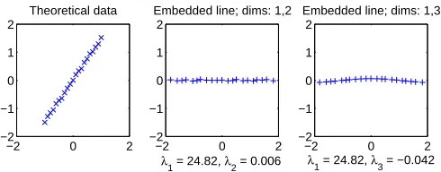
A justification for choosing only positive eigenvalues can be found in Section 3.4, where the issue of noise influence is discussed.We argue that, in general, directly measured distances may be noisy, and therefore, they may not be perfectly Euclidean, which will result in small negative eigenvalues of B; see Figure 1 for an illustration. Therefore, by disregarding them, noise can be diminished.

• It is known that there exists a positive constant c > |λ|, where λ is the smallest (negative) eigenvalue of B, such that a new square Euclidean distance matrix might be created fromD(2)by addingcto off-diagonal elements (Cox and Cox, 1995, Gower, 1986), i.e.:

D(2)_n =D(2)+c(1 1T −I). (5)

Then,X can be again expressed in an Euclidean space.In practice, the eigenvectors remain the same and the value c₂ is added to the non-zero eigenvalues, giving the new eigenvalue matrix Λk+₂cI.This is equivalent to regularizing the covariance matrix

of our configurationX, i.e. Cov(X) = _n−1₁(Λk+c₂I) and changing X respectively.

−2 0 2 −2

−1 0 1 2

Theoretical data

−2 0 2

−2 −1 0 1 2

Embedded line; dims: 1,2

λ₁ = 24.82, λ

2 = 0.006

−2 0 2

−2 −1 0 1 2

Embedded line; dims: 1,3

λ₁ = 24.82, λ₃ = −0.042

Figure 1: An example on the usefulness of disregarding the negative eigenvalues.Assume that the theoretical, original data is a perfect line, however due to the measure-ment process, somewhat distorted, as observed in the first plot.The distance kernel D is computed with distances dij = ||xi−xj||1.004, which is nearly

Eu-clidean.During the embedding process 16 eigenvalues are revealed, where 14 are negative (the largest negative in magnitude equals−0.042).This would suggest a possible 16-dimensional configuration, however, one significant positive eigenvalue indicates that the ‘real’ intrinsic dimensionality of the data is 1 (for an Euclidean distance and a perfect line, the embedded configuration is 1-dimensional).The second plot shows the projection onto first two dimensions (the configuration is retrieved up to a rotation).The last plot presents the projection onto the 1st and the 3rd dimensions, where the 3rd dimension corresponds to the largest (in magnitude) negative eigenvalue (how the embedding is done in such a case is ex-plained by Formula 8).Notice how a tiny change of both the theoretical data and the Euclidean distance of a very simple problem enlarges the number of retrieved dimensions, from 1, in the perfect case, to 16.

Another possibility exists for problems in which the Euclidean space is not ‘large enough’. Goldfarb (1984, 1985) proposed to project the data onto a pseudo-Euclidean space, which can be performed for any symmetric distance matrix.The pseudo-Euclidean space can be seen as consisting of two Euclidean spaces, for which the inner product operation is positive definite on the first space and negative definite on the second one (see Greub, 1975, Appendix Appendix A.1).For a simple illustration, see Figure 2.To embed the data, the same reasoning as for an Euclidean space is applied here.The essential difference refers to the notion of an inner product and a distance.Now,B =−1₂J D(2)J, is still the matrix of inner products, but it is expressed as (see Appendix A.1):

B =X M XT, (6)

whereM is a matrix of the inner product operation in a pseudo-Euclidean space.Following Goldfarb (1985), we can write (compare to Formula 2):

X M XT =B =QΛQT =Q|Λ|12

M 0

|Λ|12 QT, where M =

Ip×p 0

0 −Iq×q,

(7)

−4 −3 −2 −1 0 1 2 3 4 −4

−3 −2 −1 0 1 2 3 4

R(1,1) <x,y> = x

1 y1 − x2 y2 = x

T

M y

vT _{M x = 0}

v

A B C E

F

G

<x,x> < 0 <x,x> < 0

<x,x> > 0 <x,x> > 0 w = Mv

D

O

Figure 2: A pseudo-Euclidean spaceR(1,1), whered2(x,y) = (x−y)TM(x−y).Here, the length of any vector of the form [x1 ±x1]T, is zero.The orthogonal vectors are

mirrored w.r.t. the lines x2 = x1 or x2 = −x1, e.g. OA, OC = 0.Vector v

defines the plane vTMx= 0 in this space.Vector w=Mv, a ‘flipped’ version ofv, describes the plane as if in an Euclidean space, i.e. it is perpendicular. This explains that in any pseudo-Euclidean space, the inner product operation can be seen as an Euclidean operation where one vector is ‘flipped’ by M.In general, distances can be of any sign, e.g.: d2(A, C) = d2(F , G) = 0, d2(A, B) = 1, d2_{(B, C) =−1,d}2_{(D, A) =−8, d}2_{(F , A) = 21 and d}2_{(E, C) = 8.}

in a pseudo-Euclidean spaceRk_=R(p,q)_{of, the so-called, signature (p, q) (Goldfarb, 1984),}

as follows:

X=Qk|Λk| 1

2. (8)

Note that X has uncorrelated features, since the estimated pseudo-Euclidean covariance matrix (which is not positive definite as in an Euclidean space) is given as (Goldfarb, 1985):

Cov(X) = 1 n−1X

T _{X M =} 1

n−1|Λk|M = 1

n−1Λk. (9)

This means that X is a result of a mapping in the sense of the PCA projection and the whole embedding procedure can be also interpreted as a sort of a kernel-PCA (Sch¨olkopf et al., 1999, Sch¨olkopf, 2000) approach, where the kernel B is a reproducing kernel for the pseudo-Euclidean feature space (see Section 4.4).

configu-rationX, a linear classifiery=vTMx+v0 can be found by addressing it as in a standard,

Euclidean case, i.e. y=wTx+v0. 3.3 Embedding new points

Having found a configuration X in a pseudo-Euclidean space that preserves all pairwise distances D(R, R), new objects can be can added to this space via the linear projection. Given the square distance matrix Dn(2) ∈ Rs×n, expressing dissimilarities between s novel

objects and all objects of the representation setR, a configuration Xn is to be determined

in a pseudo-Euclidean space Rk _{= R}(p,q)_{.First, the matrix B}

n ∈ Rs×n of inner products

relating all new objects to all objects fromRshould be found, which becomes (see Appendix A.3):

Bn=−

1 2(D

(2)

n J−U D(2)J), (10)

whereJ is the centering matrix and U = _n11T1∈ Rs×n.Since Bn can be expressed as: XnM XT =Bn, with

M =

    

I ∈ Rk×k if the space Rk is Euclidean,

Ip×p 0

0 −Iq×q

∈ Rk×k _{if the space R}k _{is pseudo-Euclidean,} (11)

therefore, Xn is found as the mean-square error solution to XnM XT = Bn, i.e. Xn = BnX(XT X)−1M.Knowing that XTX = |Λ| and X = Qk|Λk|

1

2, Xn is alternatively

presented as:

Xn=BnX|Λ|−1M or Xn=BnQk|Λk|− 1 2 M.

3.4 Reduction of dimensionality

By adding one object to the representation set R, (and, therefore, to the dissimilarity kernelD(R, R)), in practice one point is added to a finite pseudo-Euclidean space, but the dimensionalitykof the vector representation might increase by more than one, contrary to the Euclidean case (Goldfarb, 1985).This means that both outliers and noise can contribute significantly to the resulting dimensionalityk.In practice, when new points are added, they are projected onto the space determined by the starting configuration X.Therefore, the reliability of X, i.e. whether D(R, R) describes a sufficiently well sampled representation set, plays an essential role in the process of representing new data, and consequently, the classification performance.

−10 0 10 −10

−5 0 5 10

Theoretical data A

−10 0 10

−10 −5 0 5 10

Λ’s: 5251.5, 1725.5 Based on D(A)

−10 0 10

−10 −5 0 5 10

Λ’s: 5251.5, 1725.4, 2.3,..,0.01,−2.4,..,−0.004

Based on D(A)+noise

−10 0 10

−10 −5 0 5 10

Λ’s: 5251.5, 1725.5, 0.006, 0.003 Based on D(A+noise)

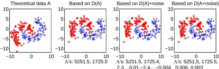
Figure 3: Noise influence on eigenvalues ofB.The first, leftmost plot presents the 2D the-oretical banana data (consisting of 200 points), for which the Euclidean distance matrixDhas been computed.The second plot shows the result of the embedding of Dinto a 2D space (note that the retrieved configuration is up to a rotation). The third plot presents the projection onto the first 2 dimensions of the 199D data obtained via embedding of distorted distances ˜D, (where ˜dij = dij +sij

and sij ∼N(0,0.001)), which become non-Euclidean.The last plot presents the

projection onto the first 2 dimensions of the 4D data obtained via embedding of D( ˜A), where ˜A consists of the theoretical data A to which 2 noisy features were added.Note that the first 2 largest eigenvalues, as given under the graphs, are about the same for non-distorted as well as for distorted data, which gives practically the same results in all cases.Therefore, by rejecting relatively small eigenvalues, noise is diminished.

In such a case, distances will be preserved approximately.One has, however, a control over the dimensionality of the reduced vector representation.Basically, the dimensional-ity reduction can be achieved by the orthogonal projection, governed by the PCA.The particular construction of X = Qk|Λk|

1

2 and the fact that X is an uncorrelated vector representation, i.e. Cov(X) = _n−1₁Λk, stand for X being given in the form of the

orthog-onal PCA projection; see Formula (9).It means that the reduction of dimensiorthog-onality is performed in a simple way by neglecting directions corresponding to eigenvalues small in magnitude.The reduced representation (being an orthogonal projection) is then deter-mined by the p significant positive eigenvalues and q significant (in magnitude) negative eigenvalues.Therefore,X ∈ Rn×k,k < k, is found as X =Qk|Λk|

1

2, where k =p+q and Λk is a diagonal matrix of first, decreasing positive eigenvalues and then increasing

negative eigenvalues, and Qk is the matrix of corresponding eigenvectors.

4. Classification in a pseudo-Euclidean space

4.1 Generalized nearest mean classifier

Nearest mean classifier (NMC) is the simplest linear classifier which assigns an unknown object to a class of the nearest mean.In a (pseudo-)Euclidean space Rk, such a decision rule is based on the (pseudo-)Euclidean distance.GivenD, assume a 2-class problem with the classesω1 and ω2.The vector representation {x1, . . . ,xn} is such that it preserves the

originally considered squared distances D(2).Let x(i) be the mean vector of the class ωi.

For a new objectz represented in this space, aszx, the classification rule is defined as:

Assignz toω1 iffd2(zx,x(1))< d2(zx,x(2))

Assignz toω2 otherwise

where d2_{(x,y) = ||x−y||}2 _{= x−y,x−y = (x−y)}T_{M(x−y) andM is defined by}

Formula (11).Embedding a dissimilarity kernel D can be avoided when only class mean vectors and distances have to be computed.Therefore, we propose an alternative approach. A similar classification process can be carried out, however, without performing the exact mapping.As a result, the generalized nearest mean classifier (GNMC) will be obtained.

Assume first that a class ω is represented by a distance matrix D(R, R) based on the representation set R={p1, . . . , pn}.Let a new objectz be represented by distances to the

set R.Then, the proximity of zto the class ω is measured by the function fω defined as:

fω(z) = _n1 n_j=1 d2(z, pj)−Vd(R), Vd(R) = _2n12 nj=1

n

k=1 d2(pj, pk),

(12)

where Vd(R) is a generalized variability of the underlying feature space.It can be shown

(see Appendix A.4) that the following holds:

fω(z) = ||zx−x||2 =d2(zx,x), Vd(X) = _n1 nj=1||xj||2− ||x||2,

(13)

where {x1, . . . ,xn} is found by a linear embedding, as introduced in Section 3 and zx is

the representation of the object zin space Rk.

From dependencies given in (13), two important observations can be made.The first one refers toVdexpressing a variability inX.IfX is a 1-dimensional vector, thenVdcoincides

with the variance ofX.For X being a higher dimensional Euclidean representation, Vd is

equal to the sum of variances, i.e. trace (cov(X)).For a pseudo-Euclidean space,Vdstands

for a generalized variability, based on the pseudo-Euclidean covariance matrix; see Formula (9).The second observation refers to the function fω(z) which measures the distance of

the point zx to the mean of the classω, both represented in the space Rk.The interesting

point is that such a distance can be computed without performing the embedding process explicitly, since it operates only on the given distancesD, as presented in (12).

This result allows us to define a generalized nearest mean classifier as follows:

Assignz toωj :fω_j(z) = min

i {fωi(z)}, (14)

wherefω_i is defined as in (12).In other words, zis assigned to a class of the nearest mean

The NMC and the GNMC in a pseudo-Euclidean space are not, in general, identical classifiers.The NMC finds a linear embedding onto a feature space Rk based on the whole distance matrixD(2).Therefore, the dimensionality of such a space is determined by both the within-class and between-class distances.The GNMC operates only on the within-class distances.Although the embedding is not performed directly, the GNMC works in the underlying feature spacesRk_ωi, for each class separately.It may happen that the signatures of feature spacesRk_ωi are not the same.In such a case, the performances of the the NMC and the GNMC differ, because the NMC unifies pseudo-Euclidean space and the signature for all classes, while the GNMC treats them separately, which allows to describe them properly. Since the GNMC makes use of the distinct signatures, its accuracy is expected to be higher for problems in which the classes behave differently.

4.2 Fisher linear discriminant

The linear classifier (or a separating hyperplane) in a pseudo-Euclidean space Rk _=R(p,q)

is defined as follows (Greub, 1975, Goldfarb, 1985):

f(x) =vT Mx+v0, where M =

Ip×p 0

0 −Iq×q

(15)

To construct the Fisher linear discriminant (FLD), the notion of a pseudo-Euclidean co-variance matrix is needed.For the representationX, it is defined as (Goldfarb, 1985):

cov(X) = 1 n−1

_n

i=1

(xi−x) (xi−x)T

M, where x= 1 n

n

i=1

xi.

Making use of the above definition and following Goldfarb (1985), the FLD, obtained by maximizing the ratio of between-scatter to within-scatter (Fisher criterion) (Fukunaga, 1990), for a 2-class problem is given by:

v = M C_W−1(m1−m2), n

v0 = −1₂(m1+m2)T M M =I

C_W−1(m1−m2),

whereCWM is the pooled within-class covariance matrix in a pseudo-Euclidean space (CW

is the pooled within-class covariance matrix as computed for the Euclidean case) and m1

andm2stand for the class means.The FLD in a pseudo-Euclidean space can be constructed

as the hyperplanef(x) =wTx+v0, wherew=Mv and wTxrefers to an Euclidean inner

product.See Figure 4 as an illustration of a simple problem.

4.3 Support vector classifier

Letnpointsxi,i= 1,2, . . . , nbe given in an Euclidean spaceRk.Each pointxi belongs to

one of two classes as described by the corresponding label yi ∈ {−1,1}.The goal for

non-overlapping classes is to find the optimal hyperplane: f(x) =wTx+w0, which maximizes

−5 0 5 −5

0 5

R2 Theoretical data

−5 0 5

−5 0 5

R(1,1) Embedding; L_0.6

−5 0 5

−5 0 5

R(1,1) Embedding; L_0.9

−5 0 5

−5 0 5

R2 Embedding; L_1.5

−5 0 5

−5 0 5

R2 Embedding; L₂

Figure 4: An illustration of the decision boundary of the FLD in an embedded space.The leftmost plot presents a 2D theoretical, artificial data.There are 3 training points, marked by circles.Only 3 objects are taken for training, because then the data can be perfectly embedded in not more than 2 dimensions.The remaining points, marked by ‘+’ and ‘*’ belong to the examples of testing data, which illustrate how the new objects are projected on the retrieved (pseudo-)Euclidean space. The following plots show the embedding results of the Lp distance D, where dij = ( 2k=1 |xik−xjk|p)1/p, forp={0.6,0.9,1.5,2}.For positivepsmaller than

1, the Lp distance is not metric and in such cases the distances between close

objects are emphasized.In all subplots, the FLD, determined by the 3 circles, in the original (first subplot) or the embedded spaces is drawn.For p = 2, the original, theoretical data is retrieved up to a rotation.

classification errors, so that the soft margin linear support vector classifier (SVC) (Vapnik, 1995, Burges, 1998) is found as the solution of the quadratic programming procedure:

Minimize 1₂wTw+C n_i=1ξi

s.t. yi(wTxi+w0)≥1−ξi, i= 1,2, . . . , n ξi ≥0

(16)

The term n_i=1ξi is an upper bound on the misclassification of the training samples and C can be regarded as a regularization parameter, a trade-off between the number of errors and the width of the margin.The dual programming formulation is given as follows:

Maximize −1₂αT diag(y)Kdiag(y)α+αT1

s.t. αT y= 0

0≤αi ≤C, i= 1,2, . . . , n

(17)

where K is an n×n kernel matrix such that Kij = xi,xj.After solving the problem

(17), the weight vector w is found to be a linear combination of the data vectors, giving w= n_i=1αiyixi.Since manyαi become zero, the data pointsxi with positiveαi, are the

so-called support vectors.Only they contribute to the hyperplane equation.As a result, the discrimination function can be presented in terms of inner products as follows:

f(x) =

α_i>0

αiyix,xi+w0. (18)

Since the linear SVC is based only on inner products, and by the linear relation (1) between D(2) and B (= K), the SVC can be easily constructed in the underlying feature space without performing the embedding explicitly, provided that the distances are Eu-clidean.For novel objects, represented by the distances to the representation set R, the SVC can be immediately tested by using Bn, the matrix of inner products between new

objects and objects embedded originally, as provided by Formula (10).

For a non-Euclidean dissimilarity matrixD, the matrix of inner products is not positive definite, resulting in a pseudo-Euclidean space, The configuration X is given by (8), i.e. X =Q|Λ|12, for which a linear classifier is defined by (15).If we now assignwT =vT M, then the classifierf(x) =wTx+v0 can be treated in an Euclidean space.The operation of

vT _{M is seen as flipping the values of thewvector in all ‘negative’ directions of the}

pseudo-Euclidean space.As suggested by Graepel et al.(1999a), this is equivalent to flipping the negative eigenvalues to positive ones, and considering the inner product B = Q|Λ|QT in an Euclidean space as being positive definite.

Summarizing, for a dissimilarity kernelD, the SVC classifier can be built in the under-lying feature space as follows.First, the matrixB is computed according to (1).IfB is not positive definite, then the matrix B is computed as B =Q|Λ|QT, otherwise B =B.It describes a positive definite kernel, used to construct the SVC according to (18).Note also that any polynomial SVC classifier (Vapnik, 1995) can be built by usingB directly.

4.4 Discussion on the kernel trick for distances

Recently, Sch¨olkopf (2000) has considered kernels as generalized dissimilarity measures.His reasoning starts from the observation that a Mercer kernelK (Vapnik, 1995), i.e. a positive definite kernel, can be seen as a (nonlinear) generalization of the similarity measure based on inner products.This is possible because such a kernel can be expressed as an inner product operation in some high-dimensional feature space G, i.e. K(x,y) = φ(x), φ(y), where φ is a mapping, φ : F → G and φ(x) is the image of x in the space G.Following the same idea, Sch¨olkopf considers a generalization of the squared Euclidean distance in the space G, by using, the so-called kernel trick:

||φ(x)−φ(y)||2=K(x,x) +K(y,y)−2K(x,y),

which allows to express this distance only by using the kernel, without explicitly performing the mapping.Next, Sch¨olkopf argues that a larger class of kernels, namely theconditionally

positive definite kernels, can be used.A symmetric function K :F × F → R which for all

m∈ N, all vectors c∈ Rm×1 and all xi∈ F fulfills:

cT _{Kc≥0, where K}

ij =K(xi,xj) (19)

is called a positive definite (p.d.) kernel. When the inequality (19) is satisfied for c such thatcT1= 0, the kernel is called conditionally positive definite (c.p.d.). A relation between the p.d. and c.p.d. kernels can be established as (‘†’ stands for a conjugate transpose):

˜

K= 1

2(I−1w

†_)K(I−w1†_{), where w1}†_{= 1 (20)}

In the simplest case,ci= _n1 for alli, (20) is then equal to Formula (1), if we readB = ˜K

and D(2) =−K.This means that D is an Euclidean distance matrix, if and only if−D(2) is a c.p.d. kernel.

For K, being a c.p.d. kernel, with K(x,x) = 0 for all x ∈ F, there exists a Hilbert space Hof real-valued functions onF and a mapping φ:F → H, such that

||φ(x)−φ(y)||2 =−K(x,y). (21)

This supports the fact that an Euclidean distance kernelDcan be embedded in an Euclidean space, which is an example of a Hilbert space.This is justified byK =−D(2) being a c.p.d. kernel.This means that in this paper a particular case of the mappingφ is considered.

More generally, Sch¨olkopf proves that for a real-valued, symmetric kernel ˜K, there exists a linear spaceH(which might not be a Hilbert space) of real-valued functions onF, endowed with a symmetric, bilinear formQ(·,·) and a mappingφ:F → H, such that

˜

K(x,y) =Q(φ(x), φ(y)).

˜

K is then a reproducing kernel for a feature spaceH (Wahba, 1999).

According to the definition, a pseudo-Euclidean space (Greub, 1975)is equipped with a non-degenerate, indefinite, symmetric bilinear form Q =·,·, seen as a generalized inner product (see Appendix A.1). This justifies that for a non-Euclidean distance kernel D,

˜

K =B = 1₂J K J, where K=−D(2) (see Formula 1), is a reproducing kernel for a pseudo-Euclidean feature spaceH.

Sch¨olkopf argues also that the c.p.d. kernels K are ‘ a natural choice whenever we are dealing with a translation invariant problem’, where the SVC or the kernel-PCA are of an example.From Formula (21) it follows that−K is the squared Euclidean distance in some Hilbert space.

In summary, Sch¨olkopf provides a new framework for distance based algorithms.The squared Euclidean distance can now be realized in another feature space by using a suitable kernel function, which should be conditionally positive definite. Using Formula (20), a c.p.d. kernel can be transformed into a p.d. kernel, to which, again, the kernel algorithms could be applied.In this way, Sch¨olkopf’s work provides a mathematical context of our approach of embedding distances. It gives more information on relations between the c.p.d. kernels and p.d. kernels, or in other words, it names the class of c.p.d. kernels that can be isometrically embedded in an Euclidean space.However, Sch¨olkopf starts from a given feature space and a known dissimilarity measure.We assume that a distance kernel is given implicitly by a dataset, maybe not even knowing what type of a measure it is or how it was computed.One of our approaches relies on a linear embedding, which is a particular case of a mapping φ considered by Sch¨olkopf.While Sch¨olkopf focuses mostly on a mathematical formulations, we try to study how the methods work in practice.

5. Classification on dissimilarities

The second approach, mentioned in the introduction, addresses the dissimilarity kernel as a mapping defined by the representation setR={p1, . . . , pn}.A mappingD(z, R) :F → Rn

0 5 10 15 −5

0 5

Theoretical data

0 5 10 0

5 10

Dissimilarity data

D(.,p 1)

D(.,p

2

)

0 5 10 15 −5

0 5

Theoretical data

0 5 10 0

5 10

Dissimilarity data

p₁

p 2

D(.,p

2

)

D(.,p 1) p₁ p

2

Figure 5: A simple illustration of a 2D dissimilarity space.The first and third plots show the theoretical, artificial data, with a quadratic classifier.TheLp distance D, where dij = ( 2k=1 |xik−yjk|5/2)2/5 was computed for this data.The representation set

consist of two objects, i.e. R= [p1, p2].The second and the fourth plots present

the dissimilarity spacesD(·, R), where the representative objects are marked by circles on the first and third plots.Note that ifRis well chosen, a linear classifier on a dissimilarity kernelD(·, R) separates the data very well.

feature space of objects, which might not be given explicitly.The dimensionality of such a dissimilarity space is controlled by the size of R.Using this formulation, classifiers can be constructed directly on the dissimilarity kernels, as in the dissimilarity space.

A justification to construct classifiers in dissimilarity space is as follows.The property that distances should be small for similar objects, i.e. belonging to the same class, and larger for objects of different classes, gives a possibility for a discrimination and, thereby, D(·, pi), defined by the distances to the representative pi, can be interpreted as a feature.

If,pi is a characteristic object of a particular class, then the discrimination power ofD(·, pi)

can be large.On the other hand, if pi is a non-typical object of its class, then theD(·, pi)

may discriminate poorly.

Defining a well-discriminating dissimilarity measure for a non-trivial recognition prob-lem is difficult.On the other hand, when a good distance measure is derived, we almost solved our classification problem.It is still a challenge, especially if such a measure should preferably incorporate invariances.Building such a measure is equivalent to defining good features for a traditional classification problem.If a good measure can be found, then the k-nearest neighbor (k-NN) method is expected to perform well provided that D is metric or nearly metric.The decision of thek-NN is based on local neighborhoods only and it is, in general, sensitive to noise.It means that k nearest neighbors found might not include the best representatives of a class to which an object should be assigned.Moreover, the k-NN does not work for an asymmetric distance measure or might perform very badly for dissimilarities which strongly do not obey the triangle inequality.In such cases, a better generalization can be achieved by a classifier built in a dissimilarity space.

built, by which its sensitivity to noisy representative examples is reduced.Our experience confirms that a linear or quadratic classifier can often generalize better than thek-NN rule, especially for a small representation set R (see (Pekalska and Duin, 2001)).

A linear classifier built on the dissimilarity kernelD is given by:

f(D(x, R)) =

n

j=1

wjd(x, xj) +w0 =wT D(x, R) +w0 (22)

and a linear classifier on the dissimilarity kernel D(2) is expressed as:

f(D(2)(x, R)) =

n

j=1

wjd2(x, xj) +w0=wTD(2)(x, R) +w0. (23)

There is an essential difference between those two separating hyperplanes.Because of the linear relation between the square distance matrix D(2) and the matrix of inner products, the classifier (23) built onD(2) is, in fact, a quadratic classifier in the underlying space.The linear classifier (22), constructed on dissimilarity kernel D, is, in general, non-quadratic, nonlinear classifier in the underlying feature space, since there is a nonlinear relation between the inner products and the kernelD.

5.1 The Fisher Linear Discriminant (FLD)

In general, any traditional classifier operating on feature spaces might be used on dissimi-larity kernels.Since most of the commonly-used dissimidissimi-larity measures are based on sums of differences between measurements, the choice of the linear Bayesian classifier, assuming normal densities, is a natural consequence of the central limit theorem applied to them.In principle, the quadratic Bayesian classifier could be even better, but it requires much more training objects for estimation of the class covariance matrices.It is known that for 2-class problems with equally probable classes, this classifier is equivalent to the Fisher linear dis-criminant (FLD), obtained by maximizing the so-called Fisher criterion, i.e. the ratio of between-scatter to within-scatter (Duda et al., 2001, Fukunaga, 1990). Therefore, we refer to this separating hyperplane as to the FLD.

The FLD can be now constructed on D in the form of (22).As a starting point, the representation set R, consisting of nobjects, and the training set T coincide, i.e. T =R. In such a case, we have to deal with a small sample size classification problem, i.e. withn vectorsD(xi, R) inndimensions.We have recently proposed to use a reduced representation

After R has been established, a linear classifier is built onD(T, R).For a new object, only distances to the set R have to be computed.For a 2-class problem, with the prior probabilities pω₁ and pω₂, the linear Bayesian classifier (Fukunaga, 1990) is constructed on

the dissimilarity kernelD as follows:

f(D(x, R)) =wT D(x, R)T +w0,

where w=C_W−1(m1−m2) andw0 = −1₂(m1+m2)T CW−1(m1−m2) +log( pω₁

pω₂). CW is

the pooled within-class covariance matrix andmi,i= 1,2, stands for the class mean in the

dissimilarity space D(·, R).

WhenT andR are identical (orR =R),CW becomes singular, and the linear classifier

cannot be built.Regularization can be used instead, yielding an approximated covariance matrix (1−λ)CW +λ I.A classifier based on the regularized covariance matrix is called

the regularized linear discriminant (RLD).

5.2 Linear programming (LP) machines

With a properly defined objective function and constraints for a dissimilarity kernel, a sep-arating hyperplane can be obtained by solving a linear programming problem.Assume a 2-class problem, with classesω1andω2of the cardinalityn1andn2, respectively, and the

la-belsyi ={1,−1}.Letf be the separating hyperplane, built for the complete representation

set R (i.e. R = T) as given by (22).Then, the simple optimization problem, minimizing the number of misclassification errorsξj, can be defined as:

Minimize n_i=1siξi

s.t. yif(D(xi, R))≥1−ξi, i= 1, . . . , n

ξi ≥0

(24)

where si = 1 for all i, or si = _n1_i depending on a class label yi.It is argued by Bennett

and Mangasarian (1992) that the latter formulation can guarantee a nontrivial solution even when mean vectors of two classes happen to be the same.Such a problem can be solved by the standard optimization methods, such as simplex algorithm or interior-point methods.Since no other constraints are included, the hyperplane is constructed in an n -dimensional dissimilarity spaceD(·, R).It is possible, however, to impose a sparse solution, by minimizing the norm L1 of the weight vector w of the hyperplane (22) i.e. ||wj||1 =

n

j=1|wj|.In order to formulate such a minimization task in terms of a LP problem (i.e.

to eliminate the absolute value |wj| from the objective function), wj is expressed by

non-negative variablesαj andβj aswj =αj−βj.The minimization problem becomes thereby:

Minimize n_i=1(αi+βi) +C ni=1ξi

s.t. yif(D(xi, R))≥1−ξi, i= 1, . . . , n

αi, βi, ξi≥0

(25)

ρbecomes a variable of the optimization problem.Note thatρ= 1 for the formulation (25). By imposing||w||1 to be constant, the modified version of (25) can be introduced as:

Minimize _n1 n_i=1ξi−µ ρ

s.t. n_i=1(αi+βi) = 1

yif(D(xi, R))≥1−ξi, i= 1, . . . , n

ξi, αi, βi, ρ≥0

(26)

In this approach, a sparse solutionw is obtained, which means that important objects are selected (by nonzero weights) from the original representation setR(R=T), resulting in a reduced setR.This solution is a similar adaptation of the SVC for feature representations defined with the LP machines (Smola et al., 1999, Sch¨olkopf et al., 2000). It is of essential importance since for novel objects only dissimilarities to the objects from R have to be computed.

5.3 Support vector classifier

The support vector classifier can be built on the dissimilarity kernel.Recall, that for a chosen representation set R ={p1, p2, . . . , pn}, a dissimilarity mapping D(z, R) :F → Rn

is defined as D(z, R) = [d(z, p1) d(z, p2) . . . d(z, pn)]T.Since the linear decision function

in such a space is given by (22), the support vector kernel K consists of the elements:

Kij =D(xi, R), D(xj, R),

where ·,· stands here for the Euclidean inner product.Therefore, in the formulation of the linear support vector classifier (see Section 4.3), the matrix K is given by K =D DT, which is positive definite and can be used for the construction of the SVC.In such a case, however, a sparse solution, provided by the method, is obtained in the whole dissimilarity space D(·, R).It means that for evaluation of new objects, still the dissimilarities to all training objects should be computed, because our SVC is in the form of (22).

6. Experiments with the NIST digits

All experiments in this section are based on a 2-class problem, i.e. the recognition of digits 3 and 8 from a NIST database (Wilson and Garris, 1992).In total, the data consist of 2000, equally sampled, 128×128 binary images.Since no features are given to describe the images, they are represented by dissimilarity kernels.

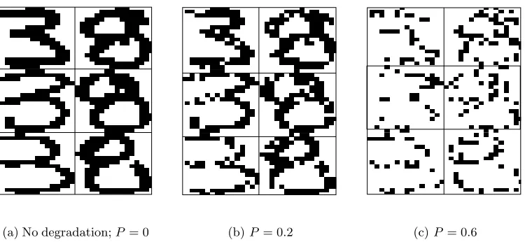
(a)No degradation;P= 0 (b)P = 0.2 (c)P = 0.6

Figure 6: Degradation of images of handwritten digits 3 and 8.Subplot a shows exam-ples of 16×16 binary digits used in our experiments.Images of degraded digits are presented in subplots b and c.The level of degradation is governed by the probabilityP that an individual pixel is set to background.

Two different dissimilarity measures are considered here: Euclidean on blurred images and modified-Hausdorff (Dubuisson and Jain, 1994) on digit contours.They were chosen to illustrate the behavior of our kernel approaches with respect to the distance properties. While the first distance is a metric, the second one is not, as it violates the triangle inequality. The modified-Hausdorff distance, applied on digit contours, is used here, since it is found useful for template matching purposes (Dubuisson and Jain, 1994).It measures the difference between two setsA={a1, . . . , ag}and B ={b1, . . . , bh}and is defined as:

DM H(A, B) = max{hM(A, B), hM(B, A)} and hM(A, B) =

1 g

a∈A

min

b∈B||a−b||.

To calculate such a distance between two images, first the digits are detected and then the dissimilarity is computed with respect to the boxes surrounding them, which means that it is shift-invariant.

To find the second dissimilarity measure, images are first blurred with the Gaussian function with the standard deviation of 8 pixels (which is similar to the distance transform of an image).The motivation for such preprocessing is to avoid sharp edges of the digits. We, thus, make our technique robust to small tilts or variable thickness.Then, the Euclidean distance is computed between the blurred versions.

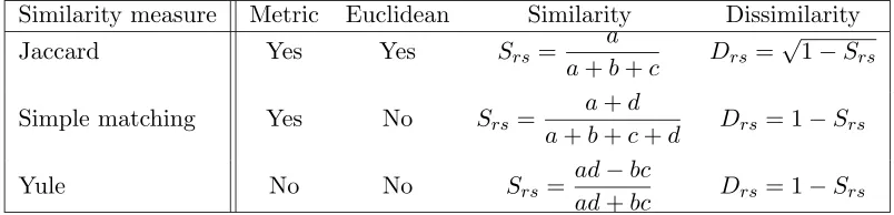
Table 1: Dissimilarity coefficients for the binary images r and s.

Similarity measure Metric Euclidean Similarity Dissimilarity

Jaccard Yes Yes Srs=

a

a+b+c Drs=

√ 1−Srs

Simple matching Yes No Srs=

a+d

a+b+c+d Drs = 1−Srs

Yule No No Srs=

ad−bc

ad+bc Drs = 1−Srs

In the second type of experiments, our goal is to study the usefulness of dissimilarity kernels for data with missing values.We think that dissimilarity kernels are designed for tackling such types of problems.In order to study the performance of classifiers as a function of the number of missing values, we simulated such data by randomly corrupting the images of 3 and 8.The level of degradation is governed by a probability P that a particular image pixel is set to the background.We used four different degradation levels in our experiments, i.e. P ={0.0,0.2,0.4,0.6}.Although this type of a procedure can be seen as introducing extra noise, it still simulates the missing values problem, since we assumed that the corrupted pixels had originally unknown values, and because the images are binary, the values can be just assigned to the background pixels.To simplify our experiment (to make the computation of distances less expensive), we used a resampled dataset, for which the original binary images were rescaled to a 16×16 raster; see Figure 6 for an illustration.

The usual way to compute dissimilarities on the binary data _{object s}

1 0

objectr 1 a b

0 c d

Figure 7: Similarity for binary images. is to construct a similarity measure first, and then, transform it

to a corresponding distance.Similarity measures for binary ob-jects sand r are often based on variablesa, b, c anddreflecting the number of elementary matches between objects (see Fig-ure 7).For instance, the variableareflects the number of cases where both objects scored 1.For our experiments, three mea-sures were chosen, yielding different properties: Jaccard, simple

matching and Yule similarities (Cox and Cox, 1995, Gower, 1986); see summary in Table 1. Jaccard measure is of interest, because it is an overlap ratio excluding all non-occurrences, and, thereby, disregarding the information on matches between background pixels.On the contrary, the simple matching measure, describing the proportion of matches to the total number of instances (pixels), might not be useful in our case.This comes from the fact that it counts matches between the background pixels, where some of them are considered as unknown.The Yule similarity is of different type, i.e.a cross-product ratio, measuring association between pixels as a predictability of one, given another.

0 50 100 150 200 250 0.02 0.04 0.06 0.08 0.1 0.12 0.14 0.16

Training size per class

Error rate

Blurred Euclidean distance

NMC; Eucl.emb. GNMC 1−NN

0 50 100 150 200 250

0.04 0.06 0.08 0.1 0.12 0.14 0.16 0.18 0.2

Training size per class

Error rate

Modified Hausdorff distance

NMC; Eucl.emb. GNMC (1) NMC; Ps−Eucl.emb. NMC; Eucl.emb. D(2)+c (2) 1−NN

1,2

(a)Nearest mean classifiers constructed in the embedded spaces

0 50 100 150 200 250

0.02 0.04 0.06 0.08 0.1 0.12 0.14 0.16

Training size per class

Error rate

Blurred Euclidean distance

FLD; Eucl.emb. SVC; Eucl.emb. 1−NN

0 50 100 150 200 250

0.04 0.06 0.08 0.1 0.12 0.14 0.16 0.18 0.2

Training size per class

Error rate

Modified Hausdorff distance

FLD; Eucl.emb. FLD; Ps−Eucl.emb. FLD; Eucl.emb. D(2)+c SVC; Eucl.emb. SVC; Ps−Eucl.emb. SVC; Eucl.emb. D(2)+c 1−NN

(b)The FLD and the SVC functions built in the embedded spaces

0 50 100 150 200 250

0.02 0.04 0.06 0.08 0.1 0.12 0.14 0.16

Training size per class

Error rate

Blurred Euclidean distance

FLD; random R RLD; R=T LP sparse, chosing R LP; R=T

SVC; R=T 1−NN

0 50 100 150 200 250

0.04 0.06 0.08 0.1 0.12 0.14 0.16 0.18 0.2

Training size per class

Error rate

Modified Hausdorff distance

FLD; random R RLD; R=T LP sparse, chosing R LP; R=T

SVC; R=T 1−NN

(c)Classifiers built on dissimilarity kernels, using the notion of the representation set

6.1 Results and discussion on kernel approaches to dissimilarities

For both dissimilarity kernels, modified-Hausdorff and blurred Euclidean, two experimental directions are considered.In the first direction, linear classifiers are built in the embedded space, while in the second one, linear classifiers were constructed in dissimilarity spaces, i.e.built directly on dissimilarity kernels.The results are presented with reference to the 1-NN rule, as the one, commonly applied to dissimilarity representations (for both distance kernels, the 1-NN rule is mostly the best among k-NN rules for largerk).

Concerning embedded spaces, three decision functions were used: the nearest mean clas-sifier, the Fisher linear discriminant and the support vector classifier.They are applied in an Euclidean space, based ononly positive eigenvalues, in a pseudo-Euclidean space and in an Euclidean space, obtained from the embedding of the ‘corrected’ dissimilarity kernel; see Formula (5).Note that the last classifier makes only sense for a pseudo-Euclidean space. For Euclidean dissimilarity measures, Euclidean and pseudo-Euclidean spaces coincide.Be-cause, in such a case, both embeddings are the same, results in the pseudo-Euclidean case are not reported.

Figure 8a presents the performance of all nearest mean classifiers with reference to the 1-NN rule.For both distance measures, it can be observed that such classifiers are not complex enough for this problem to give a good performance.They perform much worse than the 1-NN rule, especially, in the case of the modified-Hausdorff kernel.This suggests that for this dissimilarity, the classes revealed in an embedded space are not of a Gaussian shape.Concerning the pseudo-Euclidean space, the GNMC reaches a higher accuracy than the NMC, however, the NMC built in an Euclidean space, based on only positive eigenvalues behaves nearly the same as the GNMC.This indicates that the ‘negative’ directions in a pseudo-Euclidean space are not of much significance.An interesting observation is also that the nearest mean classifiers do not nearly improve their accuracy with the increase of training size larger than 50 objects per class.This indicates that this number of objects represents well the classes in the underlying feature space.

0 50 100 150 200

−100 0 100 200 300 400 500 600 700 800 900

Eigenvalues of B computed for the Euclidean blurred distances

0 50 100 150 200

−0.1 −0.05 0 0.05 0.1 0.15 0.2 0.25 0.3 0.35 0.4

Eigenvalues of B computed for the modified Hausdorff distances

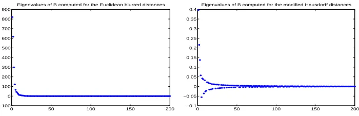
Figure 9: The eigenvalues of the matrixB of inner products for the blurred Euclidean (left) and modified-Hausdorff (right) dissimilarity kernels of the size 200×200.

were motivated by visual exploration of the eigenvalues of the inner product matrixB and selecting the number of values significantly large in magnitude (see Formulas (1)–(3)) for the embedding purpose and compare Figure 9.The results are presented in Figure 8b, for which the following conclusions can be drawn:

• For the blurred Euclidean dissimilarity kernel, both the SVC and the FLD, constructed in the embedded space, outperform the 1-NN rule.The good performance, especially of the FLD, indicates a Gaussian description of the classes (although overlapping) as revealed by original distances.

• For the modified-Hausdorff dissimilarity kernel, a linear classifier in the embedded space seems not to be complex enough, in a similar way as the NMC.The 1-NN method mostly outperforms all other decision rules considered.Note also that for the training size larger than 100 objects, the 1-NN rule here gives lower errors than the 1-NN rule on blurred Euclidean kernel.

Concerning the behavior of different variants of the FLD and the SVC for the modified-Hausdorff distances, the pseudo-Euclidean embedding allows for reaching a higher accuracy than either an Euclidean part described only by the positive eigenvalues ofB (see Formu-las 1–3) or an Euclidean embedding of the enlarged dissimilarity kernel (see Formula 5). This still shows that using the ’negative’ directions makes sense.For the embedding into Euclidean spaces, the FLD performs worse than the SVC, but in a pseudo-Euclidean space, they behave similarly.

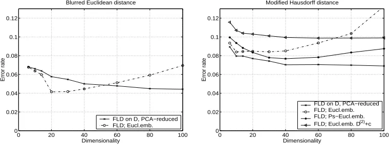
In these experiments, the results depended on the training size while the dimensionality was fixed.An additional experiment was also performed, where the training size was fixed to 100 objects per class, and the constructed dimensionality was varied.As before, the test size was set to 500 samples per class.The goal is to illustrate the performance of the FLD as a function of retrieved dimensionality.Analyzing Figure 10, the following observations can be made:

• For the blurred Euclidean dissimilarity kernel, the FLD in an embedded (Euclidean) space outperforms significantly the FLD built on the dissimilarity kernelDfor dimen-sionalities smaller than 50.The best result is reached for the dimensionality in the range 20−30.For larger dimensionalities, the error increases.Judging from Figure 9, left, we observe that there are at most 20 essential eigenvalues, since the remaining ones seem not to have a significant contribution for the FLD in the embedded space. The classifier behavior for those two error curves indicates that the classes are again linearly separable.

• For the modified-Hausdorff dissimilarity kernel, the FLD in an embedded pseudo-Euclidean space performs mostly better than the FLD in an embedded pseudo-Euclidean space.Here, however, the FLD on distance kernel D reaches the highest accuracy. This confirms that the classes can be separated best in a nonlinear way, since a linear classifier built on the dissimilarity kernel can be interpreted as a nonlinear decision function in an underlying feature space.

0 20 40 60 80 100 0

0.02 0.04 0.06 0.08 0.1 0.12

Dimensionality

Error rate

Blurred Euclidean distance

FLD on D, PCA−reduced FLD; Eucl.emb.

0 20 40 60 80 100

0 0.02 0.04 0.06 0.08 0.1 0.12

Dimensionality

Error rate

Modified Hausdorff distance

FLD on D, PCA−reduced FLD; Eucl.emb. FLD; Ps−Eucl.emb. FLD; Eucl.emb. D(2)_+c

Figure 10: The performance of the FLD for blurred Euclidean (left) and modified-Hausdorff (right) dissimilarity kernels as a function of retrieved dimensionality for the fixed training size of 100 objects per class.

distances to all representation (training) objects have to be computed for an evaluation of new objects.Therefore, the reduction of the size of R is essential from the computational point of view.

In Sections 5.1 and 5.2, two different approaches were proposed. The first possibility is to reduce R by selecting objects according to a pre-specified criterion.Here, for simplicity, the random selection of objects is used, since we found that this often gives reasonable results (Duin et al., 1999, Pekalska and Duin, 2001).In the experiments, the FLD is built on the kernelD(T, R), whereR is always randomly reduced to 25% of the training size.We also studied the RLD with the fixed regularization parameter of 0.01, constructed on the complete dissimilarity kernelD(R, R).

Another possibility is to enforce a sparse solution in a dissimilarity space in a way similar to solving the feature selection problem.This can be achieved, e.g.via linear programming schema (Bradley et al., 1998) and the classification problem can be formulated in terms of the sparse LP, as given by (26).For comparison, also an LP non-sparse solution was found, as described by (24).As a reference to all methods used, the 1-NN rule is also given.

Experimental results are presented in the Figure 8c.In case of the blurred Euclidean distances, the reduced representation sets lead to lower accuracy in comparison to the classifiers based on identical T and R.The loss in accuracy is on average 1.4%, however it is gained by using only 25% of the training samples to build R for the FLD, and by ≈15%−20% of the training samples in case of the LP formulation.The representation set Ris chosen in a different manner for these classifiers.In the case of the FLD,Ris arbitrarily chosen beforehand.For the LP, it is, on the contrary, provided as a sparse solution of the corresponding optimization task.The classification error for this method is not provided in the case of 250 training objects in Figure 8c since the minimization problem was infeasible and the solution could not be found.

For the modified-Hausdorff distances, most linear classifiers perform worse than in case of the blurred distances.The worst results are reported for the FLD based on the reduced, randomly selected R.The 1-NN rule is the best for training sizes larger than 100 objects per class.For smaller training sizes, it is outperformed, especially by the RLD and the non-sparse LP.

In summary, from this series of experiments, we can conclude that the blurred Eu-clidean dissimilarity kernel describes more compact and bounded classes than the modified-Hausdorff kernel.Also, most of the linear classifiers, both in the underlying space or on the dissimilarity kernel, perform worse in the latter case.This is probably caused by the fact, that the modified-Hausdorff distance, as applied here, does not offer rotation invariance, needed for this problem.Blurred Euclidean distance is, on the other hand, partially robust against tilting due to the initial blurring step.The 1-NN method for larger training sizes is of the best classifiers for the modified-Hausdorff case.Only the RLD and the non-sparse LP perform about the same, and for smaller training sizes, outperform the 1-NN rule.

6.2 Results and discussion on kernel approaches to dissimilarities for missing values problem

In the second track of our experiments, we studied the applicability of dissimilarity kernels to data with missing values.In order to keep a similar line of reasoning, as in the previous part, we simulated the missing values problem by setting some pixel values to the background. Both the training and testing sets have now fixed sizes and the varying quantity is the level of image degradation which was described in Section 6.

Figure 11 presents the generalization error rate as a function of increasing data degra-dation for Jaccard and Yule measures and three discussed groups of kernel methods: the variants of the NMC, the FLD and methods based on the representation set R.Since the results of the Yule measure and the simple matching dissimilarities are similar, we have cho-sen for a precho-sentation the Yule distance kernel as the distance which is both non-Euclidean and non-metric.As an indication, the most distinct results are presented in Figure 12.The following conclusions can be made in overall:

• The nearest mean classifiers are surprisingly robust against the increase of data dete-rioration, see Figure 11a.

• The FLD functions are less robust to data degradation, but they achieve higher ac-curacy than any of the NMC.

• Classifiers constructed directly on the dissimilarity kernelD, as observed in Figure 11c and 12a, generally outperform the 1-NN rule.They are also more robust against the degradation of images.Comparing all results, the 1-NN rule deteriorates the most. • Surprisingly, the performance of classifiers does not deteriorate much for increasing

image degradation.In the best cases, the error between 8%−10% is achieved for the degradation of P = 0.6 (see Figure 11 and Figure 6 for reference).It suggests that simple dissimilarity kernels based on binary images are highly robust against missing information.