SOLUTION TECHNIQUES AND ERROR ANALYSIS OF GENERAL CLASSES OF PARTIAL DIFFERENTIAL EQUATIONS

GENERAL CLASSES OF PARTIAL DIFFERENTIAL

EQUATIONS

by

Wijayasinghe Arachchige Waruni Nisansala Wijayasinghe

A thesis

submitted in partial fulfillment of the requirements for the degree of

Master of Science in Mathematics Boise State University

DEFENSE COMMITTEE AND FINAL READING APPROVALS

of the thesis submitted by

Wijayasinghe Arachchige Waruni Nisansala Wijayasinghe

Thesis Title: Solution Techniques and Error Analysis of General Classes of Partial Differential Equations

Date of Final Oral Examination: 04 March 2016

The following individuals read and discussed the thesis submitted by student Wijayasinghe Arachchige Waruni Nisansala Wijayasinghe, and they evaluated her presentation and response to questions during the final oral examination. They found that the student passed the final oral examination.

Barbara Zubik-Kowal, Ph.D. Chair, Supervisory Committee

M. Randall Holmes, Ph.D. Member, Supervisory Committee

Uwe Kaiser, Ph.D. Member, Supervisory Committee

DEDICATION

ෙමමකෘ%ෙ&

අඩං*+,ධා/තය/ෙකෙර3

උන/6ව/නාවූ,

ඇ:ම;ඇ%ව/නාවූඅයෙ<න=

සහෘදයාෙණB

ඔබටFෙම3G6ම!

My heartiest gratitude goes to my advisor, Dr. Barbara Zubik-Kowal, for her support, excellent guidance, and encouragement throughout my study. Without her continuous, valuable assistance, this would not have been a fruitful work.

I like to express my appreciation to Dr. Uwe Kaiser and Dr. Randall Holmes for their valuable suggestions and for having served on my committee.

My thanks also goes to Dr. Leming Qu, Dr. Jodi Mead, Dr. Grady Wright, Dr. Jaechoul Lee, and Dr. Marion Scheepers for helping me with my coursework and research.

Finally, I would like to thank my parents and my husband for their love and en-couragement throughout this work.

While constructive insight for a multitude of phenomena appearing in the physical and biological sciences, medicine, engineering and economics can be gained through the analysis of mathematical models posed in terms of systems of ordinary and partial di↵erential equations, it has been observed that a better description of the behavior of the investigated phenomena can be achieved through the use of functional di↵erential equations (FDEs) or partial functional di↵erential equations (PFDEs). PFDEs or functional equations with ordinary derivatives are subclasses of FDEs. FDEs form a general class of di↵erential equations applied in a variety of disciplines and are characterized by rates of change that depend on the state of the system. As opposed to traditional partial di↵erential equations (PDEs), the formulation of PFDEs, and hence, their methods of solution, are generally significantly complicated by the functional dependence of the system. Consequently, mathematical analysis has become essential to address important questions on PFDEs, their properties and solutions. This thesis is devoted to a general class of parabolic PFDEs and works out the details of the proof techniques of a related paper that help to address these questions. In particular, we examine error bounds of approximate solutions with the aim to address whether or not they converge to the exact solutions as a result of refining the associated discretizations.

ABSTRACT . . . vi

1 Introduction . . . 1

2 Numerical Solutions for a General Class of Systems of Ordinary

Functional Di↵erential Equations: Approximations and Definitions 6

3 Iterative Processes with General Splitting Functions for Semi-Discrete

Di↵erential Functional Systems . . . 10

4 Consistency Properties of Numerical Schemes for Partial Functional

Di↵erential Equations . . . 15

5 Generalized Lipschitz Conditions for Numerical Schemes Applied to

Partial Functional Di↵erential Equations . . . 24

6 Theorems on Error Bounds for Numerical Solutions to General

Par-tial Functional Di↵erenPar-tial Equations . . . 30

REFERENCES . . . 52

APPENDIX . . . 55

CHAPTER 1

INTRODUCTION

Many real-life problems can be adequately modeled in terms of systems of di↵erential equations, creating a general class into which all ordinary and partial di↵erential equations fall. A variety of models written in terms of di↵erential equations feature the independent time variablet, which plays a significant role in predicting the future behavior of certain phenomena in question with the aid of a variety of di↵erent available data, such as clinical, experimental, or field data. Although it is collected in a limited period of time, this data can be used in tandem with systems of di↵erential equations to provide information about the future.

broadly applied in many scientific disciplines such as biology, medicine, physics, engi-neering, economics, etc. Throughout its long history, functional di↵erential equations have been investigated by many authors with respect to a multitude of aspects, about which we refer the reader to [1], [2], [5]-[10], [12], [14]-[21], [23]-[28], [30], [31], [38] for ordinary functional di↵erential equations and [3], [4], [11], [13], [22], [29]-[38] for partial functional di↵erential equations. Aspects connected with modeling with functional di↵erential equations are presented in [3], [4], [13], [14], [24]. One of the main problems is that many of the equations have no analytical formulae for the exact solutions and it has become essential to study their approximations in order to gain insight about the solutions to the model equations and to conduct numerical simula-tions. In order to get reliable approximate solutions, careful mathematical analysis of their errors has to be conducted. In this thesis, we expand on the development of [37] by filling in the details of the proofs to investigate errors of approximate solutions to a class of parabolic partial functional di↵erential equations. For similar developments and proof techniques for partial functional di↵erential equations as well as numerical experiments for this class of equations, we refer the reader to [4, 22, 34, 35, 36, 38].

Originating from a multitude of areas of application to the real world around us, partial functional di↵erential equations form a general class of problems that includes partial di↵erential equations as one if its subclasses.

This thesis is devoted to partial functional di↵erential equations written in the form

@u

@t(x, t) =f ⇣

x, t, u(x,t),

@u @x(x, t),

@2_u

@x2(x, t)

⌘

, (1.1)

function. Another generalization in (1.1) is introduced by the argumentu(x,t); for any

fixedx2[ L, L] andt2[0, T],u(x,t) is a function. Such a functional argument allows

to generate di↵erential equations with e.g. a time delay and shift in space. Unlike for classical partial di↵erential equations, the third argumentu(x,t) in (1.1) is not a real

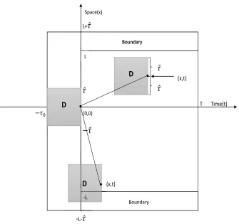
value but a real function defined on D (see Figure 1 for D) and called a functional argument. The functional argument u(x,t) 2 C(D,R) for x 2 [ L, L], t 2 [0, T], and

u₂C(B,R), withL, T > 0,B = [ ˆL,L]ˆ _⇥[ ⌧0, T],D= [ ˆ⌧,⌧ˆ]⇥[ ⌧0,0], ˆ⌧,⌧0 0,

ˆ

L=L+ ˆ⌧, is defined as

u(x,t)(s,⌧) = u(x+s, t+⌧), (s,⌧)2D.

Equation (1.1) is supplemented with the following initial conditon

u(x, t) =u0(x, t), t2[ ⌧0,0], x2[ ˆL,L],ˆ (1.2)

and boundary condition

u(x, t) = g(x, t), t2[0, T], x2[ ˆL, L][[L,L].ˆ (1.3)

Here, f : [ L, L]⇥[0, T]⇥C(D,R)⇥R⇥R !R is a continuous function, and u0, g are given initial and boundary functions, respectively.

The partial di↵erential equation (1.1) describes a general class of problems. For example, if f is defined by

f(x, t, , p, q) =✏q+ (0,0)(1 (0, ⌧0)), (1.4)

@u

@t(x, t) =✏ @2_u

@x2(x, t) +u(x, t)(1 u(x, t ⌧0)).

Here, the functional argument is given by t ⌧0. Another class of examples can be

generated by defining f by

f(x, t,!, p, q) = a(t)q+a(t) Z 0

⌧0

Z ˆ⌧

ˆ

⌧

!(s,⌧)dsd⌧, (1.5)

where a2C([0, T],R+). Then, (1.1) can be written in the general form

@u

@t(x, t) =a(t) @2_u

@x2(x, t) +a(t)

Z 0

⌧0

Z ⌧ˆ

ˆ

⌧

u(x+s, t+⌧)dsd⌧.

An important subclass of the class of partial functional di↵erential equations captured by (1.1) that may be most familiar to most readers is the entire class of partial di↵erential equations written in the form

@u

@t(x, t) = ˜f ⇣

x, t, u(x, t),@u @x(x, t),

@2_u

@x2(x, t)

⌘ ,

where ˜f : [ L, L]⇥[0, T]⇥R3 _{! R is any given function. This entire subclass is}

another example that can be generated from the general class of equations (1.1) by suitably defining f appearing on the right-hand side.

We have seen that not only do partial functional di↵erential equations o↵er a mod-eling approach that more realistically portrays a wide class of real-world phenomena, but also that their generality encompasses wide classes of subproblems, some of which many readers have been acquainted with already in various real-world contexts.

Space(x)

L+𝜏̂

𝜏̂

T Time(t)

−𝜏0 (0,0)

−𝜏̂

D

D

-L

D 𝜏̂

𝜏̂

(x,t)

(x,t)

-L-𝜏̂

L

Boundary

Boundary Boundary

CHAPTER 2

NUMERICAL SOLUTIONS FOR A GENERAL CLASS OF

SYSTEMS OF ORDINARY FUNCTIONAL

DIFFERENTIAL EQUATIONS: APPROXIMATIONS AND

DEFINITIONS

The general class of equations given by (1.1) is written in terms of arbitrary functions f and, in many cases, analytic solutions to these equations defined in the continuum sense are unknown and approximated by numerical solutions computed on discrete subsets. For any element of any of the discrete subsets (such elements are referred to as grid-points), there exists an open neighborhood that is disjoint from the other grid-points. The discrete subsets are finite and determined by parameters, a↵ecting the coarseness of the corresponding discretizations. In the literature, the process of semi-discretization has been also referred to as the Method of Lines. Letting the values of these parameters approach zero causes the corresponding discretizations to become finer. The goal of the thesis is to study error bounds of the approximate solutions defined on the discrete subsets and to address the question of whether or not they get closer to the exact solutions as the discretization becomes finer – a property desired of discretization.

the spatial derivatives in (1.1) by discrete operators. Let the spatial step-size h > 0 and M, ˆM be such that M h=L, ˆM h= ˆ⌧ and M,Mˆ 2N. Then, we define xj =jh,

for j = 0,±1,±2, ..,±M˜, where ˜M =M + ˆM. Henceforth, we also use the notation M0 =M 1 and n = 2M 1.

For each discretization parameterh, we define the vector functionF = (F M0, . . . , FM0) : [0, T]_⇥Rn_⇥C([ ⌧0,0],Rn) ! Rn, the initial function ˜u0 : [ ⌧0,0] ! Rn, and the

initial value problem 8 > < > :

˙ (t) = F(t, (t), t), t2[0, T],

(t) = ˜u0(t), t 2[ ⌧0,0],

(2.1)

whose solution (t)2Rn _{depends onhand (as it will be shown in the next chapters)}

converges to (u(x _M0, t), ..., u(x_M0, t)), as h ! 0. Note that n ! 1, as h !0, and that the dimension of the system (2.1) increases as the discretization becomes finer.

The third input t2C([ ⌧0,0],Rn) in (2.1) is defined by

t(⌧) = (t+⌧),

for ⌧ ₂[ ⌧0,0], where t2[0, T] and 2C([ ⌧0, T],Rn).

The vector function F in (2.1) can be defined as follows

Fi(t, z,!) = f(xi, t,Li,t!, i,tz, 2i,tz), (2.2)

wherei= 0,±1, ...,±M0,t 2[0, T],z 2Rn_{, and! = (!}

M0, ...,!M0)2C([ ⌧0,0],Rn).

[Li,t!](s,⌧) =

xk+1 s

h !

t

k+i(⌧) +

s xk

h !

t

k+1+i(⌧),

where s₂[ ˆ⌧,⌧ˆ],⌧ ₂[ ⌧0,0], and k 2Nis such that xk6s 6xk+1 and

!_jt(⌧) = 8 > < > :

!j(⌧), for j = 0,±1, ...,±M0,

g(xj, t+⌧), for j =±M, . . . ,±M ,˜

whereg is defined in (1.3). The discrete operators i,t and i,t2 in (2.2) are defined for

t₂[0, T],i= 0,_±1, ...,_±M0, and z = (z M0, ..., zM0)2Rn, by

i,tz =

zt

i+1 zit 1

2h , (2.3)

2 i,tz =

zt

i+1 2zit+zit 1

h2 , (2.4)

where the vector zt= (zt_M, ...z_Mt )₂Rn+2 is defined by

z_it = 8 > < > :

g(xi, t), for i=±M,

zi, for i= 0,±1, . . . ,±(M 1).

As it will be shown in Chapter 4, the operators (2.3) and (2.4) approximate the first and second order derivatives (respectively) at the point xi.

The initial function ˜u0 : [ ⌧0,0]!Rn in (2.1) is defined by

˜

u0(t) = (u0(x M0, t), . . . , u₀(x_M0, t)),

for t ₂ [ ⌧0,0], where u0 : [ ˆL,L]ˆ ⇥[ ⌧0,0]! R is the initial function given in the

(t) 2Rn _{to (2.1) converge, as h ! 0, to the values u(x}

i, t) of the exact solution to

CHAPTER 3

ITERATIVE PROCESSES WITH GENERAL SPLITTING

FUNCTIONS FOR SEMI-DISCRETE DIFFERENTIAL

FUNCTIONAL SYSTEMS

In this chapter, we construct iterative procedures for solving the general problem (2.1) and thus (1.1)–(1.3). The process is summarised in the form of the following algorithm. Let (0) : [ ⌧0, T]!Rn be an arbitrary function. We define the sequence

of vector functions (k) : [ ⌧0, T]!Rn, where k= 0,1,2, . . ., recursively, by

˙(k+1)(t) = G(t, (k+1)(t), (k)(t), _t(k)), t₂[0, T],

(k+1)_{(t) = ˜u}

0(t), t2[ ⌧0,0].

(3.1)

The functionsGare chosen according to the givenF and are referred to assplitting functions. The function (0) is referred to as a starting function, and the functions

(k) _{are referred to as the successive iterates.}

For example, if Gis defined by

Gi(t,⇣, z, w) = Fi(t, z1, . . . , zi 1,⇣i, zi+1, . . . , zn, w),

fori= 1,2, . . . , n, where Fi is defined, for example, by (2.2), then (3.1) generates the

˙_i(k+1)(t) =Fi

⇣

t, ₁(k)(t), ..., _i(k)₁, _i(k+1)(t), (k)_i+1(t), ..., (k)_n (t), t(k)

⌘

(3.2)

or if Gis defined by

Gi(t,⇣, z, w) =Fi(t,⇣1, . . . ,⇣i, zi+1, . . . , zn, w),

then (3.1) generates another iterative process of the Picard type in the functional sense

˙_i(k+1)(t) =Fi

⇣

t, ₁(k+1)(t), ..., _i(k+1)₁ (t), _i(k+1)(t), (k)_i+1(t), ... _n(k)(t), (k)_t ⌘. (3.3)

A common feature of these two processes is that the functional argument in F is given by the previous iterate denoted by the superscriptk, as is the case for standard Picard iterations. The first of these processes has been referred to in the literature also by terms such as Jacobi-Picard scheme, Jacobi-Picard waveform relaxation scheme, Jacobi-Picard waveform method, Jacobi-Picard iteration scheme, or simply Jacobi

waveform relaxation. The second of these processes has been referred to in the literature also by terms such as Gauss-Seidel-Picard scheme, Gauss-Seidel-Picard waveform relaxation scheme, Picard waveform method,

indices of the successive iterates, and one may be preferable to the other depending on the problem.

In our error analysis, we will use the following definitions:

e(t) =U(t) (t), e(k)(t) = (t) (k)(t), E(k)(t) =U(t) (k)(t),

where t ₂ [ ⌧0, T], k = 0,1, . . ., U(t) = U1(t), . . . , Un(t) , Ui(t) = u(xi, t), and

the functions u(x, t), v(t), v(k)(t) are solutions to the three problems (1.1)–(1.3), (2.1), (3.1), respectively. Notice that e(t) is the error of semi-discretization (2.1) and e(k)(t) is the error of iterative process (3.1), while E(k)(t) is the error of both the semi-discretization (2.1) and iterative process (3.1). The prefix semi indicates that the discretization corresponds to the spatial variable only. As mentioned earlier, another name for the process of semi-discretization is the Method of Lines.

Henceforth, we will use the following assumptions. Suppose that, for

F : [0, T]_⇥Rn_⇥C([0, T],Rn)_!Rn,

there exist positive continuous functions n 2C([0, T],R+) such that

lim

n!1 n(t) = 0 (3.4)

and

˙

Ui(t) Fi(t, U(t), Ut)  n(t), (3.5)

of 4-times continuously di↵erentiable funtions from B to R) and that for the given function

f : [ L, L]⇥[0, T]⇥C(D,R)⇥R⇥R!R,

there exist positive continuous functions 1,2,3 2C([0, T],R+) such that

|f(x, t,!, p, q) f(x, t,!¯,p,¯ q)¯_{| } 1(t)|p p¯|+2(t)|q q¯|

+ 3(t) max

(s,⌧)2D|!(s,⌧) !¯(s,⌧)|,

(3.6)

for all x2[ L, L],t 2[0, T],!,!¯ 2C(D,R),p, q,p,¯ q¯2R.

For the iterative processes applied to (2.1), we assume that the functions

G: [0, T]⇥Rn_⇥Rn_{⇥C([ ⌧}

0,0],Rn)!Rn

satisfy

G(t, r(t), r(t), rt) = F(t, r(t), rt), (3.7)

for allt₂[0, T],r ₂C([ ⌧0, T],Rn) (note that for anyt2[0, T],rt2C([ ⌧0,0],Rn))

and there exist continuous functionsµ1 2C([0, T],R),µ2, µ3 2C([0, T],R+) such that

k& &¯ "[G(t,&, z,!) G(t,&¯, z,!)]_kn (1 "µ1(t))k& &¯kn, (3.8)

kG(t,&, z,!) G(t,&,z,¯ !)_kn µ2(t)kz z¯kn, (3.9)

kG(t,&, z,!) G(t,&, z,!¯)knµ3(t)k! !¯k0n, (3.10)

for " 0,t2[0, T],&,&¯, z,z¯2Rn_{,!,!¯ 2C([ ⌧}

0,0],Rn), where k·kn is an arbitrary

k!k0

n= max

⌧2[ ⌧0,0]k!(⌧)kn,

for !2C([ ⌧0,0],Rn).

CHAPTER 4

CONSISTENCY PROPERTIES OF NUMERICAL

SCHEMES FOR PARTIAL FUNCTIONAL

DIFFERENTIAL EQUATIONS

In this chapter, we present results that we will apply to derive error bounds for numer-ical solutions to partial functional di↵erential equations. In the theorem below, the notation C(4)(B,R) refers to the class of 4-times continuously di↵erentiable functions fromB toR.

Theorem 4.1 ([37], Lemma 3.1). If u 2 C(4)(B,R) and f satisfies condition (3.6), then F defined by (2.2) satisfies condition (3.5) with

n(t) =

c

n2 1(t) +2(t) +3(t) , (4.1)

for t2[0, T], where cis a positive constant that is independent on n.

˙

Ui(t) Fi(t, U(t), Ut) =

@u

@t(xi, t) Fi(t, U(t), Ut) = f⇣xi, t, u(xi,t),

@u @x(xi, t),

@2_u

@x2(xi, t)

⌘

Fi t, U(t), Ut

= f⇣xi, t, u(xi,t), @u @x(xi, t),

@2_u

@x2(xi, t)

⌘

f xi, t,Li,tUt, i,tU(t), i,t2 U(t) .

Hence

˙

Ui(t) Fi(t, U(t), Ut)  1(t)

@u

@x(xi, t) i,tU(t) + 2(t)

@2_u

@x2(xi, t) 2 i,tU(t)

+ 3(t) max

(s,⌧)2D u(xi,t)(s,⌧) Li,tUt(s,⌧) .

(4.2)

By Taylor’s Theorem applied to u(xi+1, t) and u(xi 1, t), since u 2 C(4)(B,R), we

have,

u(xi+1, t) = u(xi, t) +

h 1! ·

@u

@x(xi, t) + h2

2! · @2_u

@x2(xi, t) +

h3

3! · @3_u

@x3(✓i, t), (4.3)

with ✓i 2(xi, xi+1), and

u(xi 1, t) = u(xi, t)

h 1! ·

@u

@x(xi, t) + h2

2! · @2_u

@x2(xi, t)

h3

3! · @3_u

@x3(⇠i, t), (4.4)

@u

@x(xi, t) i,tU(t) = @u @x(xi, t)

Ui+1(t) Ui 1(t)

2h = @u

@x(xi, t)

u(xi+1, t) u(xi 1, t)

2h

= @u @x(xi, t)

1 2h

✓

2h· @u

@x(xi, t) + h3

6 · @3_u

@x3(✓i, t) +

h3

6 · @3_u

@x3(⇠i, t)

◆

= h

2

12 @3_u

@x3(✓i, t) +

@3_u

@x3(⇠i, t) .

Since u2C(4)(B,R), there exists a constant C >0 such that

@3_u

@x3(x, t) C,

for all (x, t)₂B, and

@u

@x(xi, t) i,tU(t)  Ch2

6 .

From this andn+ 1 = 2L

h , we get @u

@x(xi, t) i,tU(t)  C

6 · 4L2

(n+ 1)2 <

2CL2

3n2 . (4.5)

For the second term of (4.2), we obtain

@2_u

@x2(xi, t) 2

i,tU(t) =

@2_u

@x2(xi, t)

Ui+1(t) 2Ui(t) +Ui 1(t)

h2

= @

2_u

@x2(xi, t)

u(xi+1, t) 2u(xi, t) +u(xi 1, t)

h2

(4.6)

u(xi+1, t) = u(xi, t) +

h 1! ·

@u

@x(xi, t) + h2

2! · @2_u

@x2(xi, t) +

h3

3! · @3_u

@x3(xi, t)

+ h

4

4! · @4_u

@x4(˜✓i, t),

u(xi 1, t) = u(xi, t)

h 1!·

@u

@x(xi, t) + h2

2! · @2_u

@x2(xi, t)

h3

3! · @3_u

@x3(xi, t)

+ h

4

4! · @4_u

@x4( ˜⇠i, t),

(4.7)

with ˜✓i 2(xi, xi+1) and ˜⇠i 2(xi 1, xi), respectively. From (4.6) and (4.7), we have

@2_u

@x2(xi, t) 2 i,tU(t)

= @

2_u

@x2(xi, t)

1 h2

✓ h2@

2_u

@x2(xi, t) +

h4

24 @4_u

@x4(˜✓i, t) +

h4

24 @4_u

@x4( ˜⇠i, t)

◆

= h

2

24 @4_u

@x4(˜✓i, t) +

@4_u

@x4( ˜⇠i, t) .

Since u₂C(4)_{(B,R), there exists a constant C >0 such that}

@4_u

@x4(x, t) C,

for all (x, t)2B. From this and h= 2L

n+ 1, we get

@2_u

@x2(xi, t) 2

i,tU(t) 

Ch2

12 =

4L2_C

12(n+ 1)2 <

L2_C

3n2 . (4.8)

u(xi,t)(s,⌧) [Li,tUt](s,⌧) = u(xi+s, t+⌧)

(xk+1 s)

h ·(Ut)

t k+i(⌧)

(s xk)

h ·(Ut)

t

k+1+i(⌧),

(4.9)

for (s,⌧) ₂ D and k ₂ N such that xk  s  xk+1. Since (Ut)tj(⌧) = (Ut)j(⌧) =

Uj(t+⌧) =u(xj, t+⌧), for j =k+i and j =k+ 1 +i, from (4.9), we get

u(xi,t)(s,⌧) [Li,tUt](s,⌧)

= u(xi+s, t+⌧)

(xk+1 s)

h u(xk+xi, t+⌧)

(s xk)

h u(xk+1+xi, t+⌧)

and, by Taylor’s Theorem, we obtain

u(xi,t)(s,⌧) [Li,tUt](s,⌧)

= u(xi+s, t+⌧)

(xk+1 s)

h "

u(xi+s, t+⌧) +

(xi+xk xi s)

1!

@u

@x(xi+s, t+⌧)

+(xi+xk xi s)

2

2!

@2_u

@x2(ˆ✓i, t+⌧)

#

(s xk)

h "

u(xi+s, t+⌧)

+(xi+xk+1 xi s) 1!

@u

@x(xi+s, t+⌧) +

(xi+xk+1 xi s)2

2!

@2_u

@x2( ˆ⇠i, t+⌧)

#

= u(xi+s, t+⌧)

"

1 xk+1 s h

s xk

h #

@u

@x(xi+s, t+⌧) "

xk+1 s

h (xk s) +

s xk

h (xk+1 s) #

@2_u

@x2(ˆ✓i, t+⌧)

(xk s)2

2

(xk+1 s)

h

@2_u

@x2( ˆ⇠i, t+⌧)

(s xk)

h

(xk+1 s)2

Upon rearranging this and using the inequality

@2_u

@x2(x, t) C,

with C >0, we get

u(xi,t)(s,⌧) [Li,tUt](s,⌧)  C 2h

"

(xk s)2(xk+1 s) + (s xk)(xk+1 s)2

#

 C

2h "

h2_(x

k+1 s) +h2(s xk)

#

= Ch

2 "

xk+1 s+s xk

# = Ch

2

2

Therefore, sinceh= 2L

n+ 1, we get

u(xi,t)(s,⌧) [Li,tUt](s,⌧) 

2CL2

(n+ 1)2 <

2CL2

n2 . (4.10)

From (4.2), (4.5), (4.8), and (4.10), we get

|U˙i(t) Fi(t, U(t), Ut)|  1(t)

2CL2

3n2 +2(t)

CL2

3n2 +3(t)

2CL2

n2 ,

which shows that (3.5) holds with, for example, c= 2CL2 in (4.1), and finishes the proof.

Corollary 4.1 ([37], Corollary 3.1). Suppose that there exists a constant d >0 such that

where u is a solution of equation (1.1) with f defined by (1.4) for a class of functions

w2C(D,R)such thatmax{|w(s,⌧)|: (s,⌧)2D}d. Then the function f satisfies condition (3.6). Moreover, if u is of classC4(B,R), then F defined by (2.2) satisfies condition (3.5).

Proof. In order for Theorem 4.1 to be applied, it suffices to show (3.6). Let x ₂ [ L, L], t₂ [0, T], w,w¯ ₂C(D,R), p, q,p,¯ q¯₂R be arbitrary. From the definition of f, we get

f(x, t, w, p, q) f(x, t,w,¯ p,¯ q)¯

="q+w(0,0) 1 w(0, ⌧0) "q¯ w(0,¯ 0) 1 w(0,¯ ⌧0)

="(q q) +¯ w(0,0) w(0,¯ 0) w(0,0)w(0, ⌧0) +w(0,0) ¯w(0, ⌧0)

w(0,0) ¯w(0, ⌧0) + ¯w(0,0) ¯w(0, ⌧0)

="(q q) +¯ w(0,0) w(0,¯ 0) w(0,0) w(0, ⌧0) w(0,¯ ⌧0)

¯

w(0, ⌧0) w(0,0) w(0,¯ 0) .

and

|f(x, t, w, p, q) f(x, t,w,¯ p,¯ q)¯_|

"_|q q¯_|+ w(0,0) w(0,¯ 0) + w(0,0) _· w(0, ⌧0) w(0,¯ ⌧0)

+ ¯w(0, ⌧0) · w(0,0) w(0,¯ 0)

 "_|q q¯_|+⇣1 + ¯w(0, ⌧0) + w(0,0)

⌘ max

(s,⌧)2D w(s,⌧) w(s,¯ ⌧)

 "_|q q¯_|+ (1 + 2d) max

(s,⌧)2D w(s,⌧) w(s,¯ ⌧) .

1(t) = 0, 2(t) =", 3(t) = 1 + 2d.

We now apply Theorem 4.1 and conclude that F defined by (2.2) satisfies (3.5) with

n(t) =

c

n2("+ 1 + 2d),

which finishes the proof.

Corollary 4.2 ([37], Corollary 3.2). Let d >0 be as in Corollary 4.1 with f defined by (1.5). Then f satisfies condition (3.6). Moreover, if u is of class C4(B,R), then F defined by (2.2) and (1.5) satisfies condition (3.5).

Proof. We apply Theorem 4.1 with f defined by (1.5). Let x ₂ [ L, L], t ₂ [0, T], !,!ˆ ₂C(D,R), p, q,p,ˆ qˆ₂R be arbitrary. Since a is a positive function, from (1.5), we get

|f(x, t,!, p, q) f(x, t,!ˆ,p,ˆ q)ˆ|= a(t)q+a(t) Z 0

⌧0

Z ⌧ˆ

ˆ

⌧

!(s,⌧)dsd⌧

a(t)ˆq a(t) Z 0

⌧0

Z ⌧ˆ

ˆ

⌧

ˆ

!(s,⌧)dsd⌧

a(t)|q qˆ|+a(t) Z 0

⌧0

Z ⌧ˆ

ˆ

⌧

(!(s,⌧) !ˆ(s,⌧))dsd⌧

a(t)|q qˆ|+a(t) Z 0

⌧0

Z ⌧ˆ

ˆ

⌧|

!(s,⌧) !ˆ(s,⌧)|dsd⌧

a(t)_|q qˆ_|+a(t) Z 0

⌧0

Z ⌧ˆ

ˆ

⌧

max

(s,⌧)2D|!(s,⌧) !ˆ(s,⌧)|dsd⌧

=a(t)_|q qˆ_|+a(t) max

(s,⌧)2D|!(s,⌧) !ˆ(s,⌧)|

Z 0

⌧0

Z ⌧ˆ

ˆ

⌧

dsd⌧

=a(t)|q qˆ|+ 2ˆ⌧ ⌧0a(t) max

which shows that f satisfies (3.6) with

1(t) = 0, 2(t) = a(t), 3(t) = 2ˆ⌧ ⌧0a(t).

By Theorem 4.1, the function F defined by (2.2) satisfies (3.5) with

n(t) =

c a(t)

n2 (1 + 2⌧0⌧ˆ)

and the proof is finished.

CHAPTER 5

GENERALIZED LIPSCHITZ CONDITIONS FOR

NUMERICAL SCHEMES APPLIED TO PARTIAL

FUNCTIONAL DIFFERENTIAL EQUATIONS

In this chapter, we will show that the iterations (3.2) of the Picard type in the functional sense satisfy conditions (3.7)–(3.10), which will be useful in deriving error bounds for the general numerical schemes (2.1) and (3.1). The proof for iterations of the type (3.3) is similar.

The main result can be summarised by the following theorem.

Theorem 5.1 ([37], Lemma 3.2). Suppose that f satisfies condition (3.6) and

@f

@q(x, t,!, p, q) 0, (5.1)

where x 2 [ L, L], [0, T], ! 2 C(D,R), p, q 2 R. Moreover, suppose that ⌫ 2 C([0, T],R) is a function such that

⌫(t)_ @f

@q(x, t,!, p, q) (5.2)

Gi(t,&, z,!) = f

✓

xi, t,Li,t!,

zt

i+1 zit 1

2h ,

zt

i+1 2&i+zit 1

h2

◆

satisfies condition (3.7). Moreover, if additionally _k·kn is the infinity norm, then G

satisfies conditions (3.8)–(3.10).

Proof. First, we apply the definition of Gi and (2.2), obtaining

Gi(t, r(t), r(t), rt) = f

⇣

xi, t,Li,trt,

ri+1(t) ri 1(t)

2h ,

ri+1(t) 2ri(t) +ri 1(t)

h2

⌘

=f⇣xi, t,Li,trt, i,tr(t), i,t2 r(t)

⌘

=Fi(t, r(t), rt),

where t2[0, T] and r2C([ ⌧0, T],R) are arbitrary. This shows that (3.7) holds.

In order to prove (3.8), we begin by using the definition of Gi and then we apply

the mean value theorem

Gi(t,&, z,!) Gi(t,&¯, z,!) = f

⇣

xi, t,Li,trt,

zt

i+1 zit 1

2h ,

zt

i+1 2&it+zit 1

h2

⌘

f⇣xi, t,Li,trt,

zt

i+1 zit 1

2h ,

zt

i+1 2¯&it+zit 1

h2

⌘

= @f @q(Q)

⇣_zt

i+1 2&it+zti 1

h2

zt

i+1 2¯&it+zti 1

h2

⌘

= 2(&

t i &¯it)

h2

@f @q(Q) =

2(&i &¯i)

h2

@f @q(Q),

wheret₂[0, T],&,&¯, z ₂Rn,! ₂C([ ⌧0,0],Rn) andQ2[ L, L]⇥[0, T]⇥C(D,R)⇥

R2_{. From (5.1), we get}

@f

&i &¯i " Gi(t,&, z,!) Gi(t,&¯, z,!) = 1 +

2" h2

@f

@q(Q) &i &¯i = 1 + 2"

h2

@f

@q(Q) &i &¯i ,

where " 0. Upon taking the infinity norm on both sides of the above equation, we deduce that

& &¯ " G(t,&, z,!) G(t,&¯, z,!)

n = 1 +

2" h2

@f

@q(Q) & &¯ n.

From this and (5.2), we obtain

& &¯ " G(t,&, z,!) G(t,&¯, z,!)

n 1 +

2"⌫(t)

h2 & &¯ n

= 1 "µ1(t) & &¯ _n,

with

µ1(t) =

2⌫(t) h2 ,

which shows that (3.8) holds.

In order to prove (3.9), we apply (3.6) and obtain

Gi(t,&, z,!) Gi(t,&,z,¯ !) = f

⇣

xi, t,Li,t!,

zi+1t zit 1

2h ,

zi+1t 2&i+zit 1

h2

⌘

f⇣xi, t,Li,t!,

¯ zt

i+1 z¯it 1

2h ,

¯ zt

i+1 2&i+ ¯zit 1

h2

 1(t)

zt

i+1 zit 1

2h

¯ zt

i+1 z¯it 1

2h +2(t) zt

i+1 2&i+zit 1

h2

¯ zt

i+1 2&i+ ¯zit 1

h2

 _2h1(t)⇣|z_i+1t z¯_i+1t _|+_|z_it ₁ z¯_it _1|⌘+2(t) h2

⇣

|z_i+1t z¯_i+1t _|+_|z_it ₁ z¯_it _1|⌘

= ⇣1(t) 2h +

2(t)

h2

⌘⇣

|zi+1t z¯i+1t |+|zit 1 z¯ti 1|

⌘

where t2[0, T], &, z,z¯2Rn_{,! 2C([ ⌧}

0,0],Rn). Since

1(t)

2h + 2(t)

h2 0,

upon taking the infinity norm (withi= 1, . . . , n) on both sides of the above inequality, we get

kG(t,&, z,!) G(t,&,z,¯ !)_kn  2

1(t)

2h + 2(t)

h2

!

kz z¯_kn,

which shows that (3.9) holds with

µ2(t) = 2

1(t)

2h + 2(t)

h2

! .

In order to prove (3.10), we apply (3.6) with 1(t) =2(t) = 0 and obtain

Gi(t,&, z,!) Gi(t,&, z,!¯) = f

⇣

xi, t,Li,t!,

zt

i+1 zit 1

2h

zt

i+1 2&i+zit 1

h2

⌘

f⇣xi, t,Li,t!¯,

zt

i+1 zit 1

2h

zt

i+1 2&i+zit 1

h2

⌘

 3(t) max

(s,⌧)2D Li,t!(s,⌧) Li,t!¯(s,⌧) ,

for t 2 [0, T], &, z 2 Rn_{, !,!¯ 2 C([ ⌧}

operator Li,t we get

Li,t!(s,⌧) Li,t!¯(s,⌧) = Li,t(! !¯)(s,⌧)

= xk+1 s h

⇣

!_k+it (⌧) !¯_k+it (⌧)⌘+s xk h

⇣

!t_k+i+1(⌧) !¯_k+i+1t (⌧)⌘,

where xks xk+1, and

Li,t!(s,⌧) Li,t!¯(s,⌧) 

xk+1 s

h !

t

k+i(⌧) !¯k+it (⌧)

+s xk h !

t

k+i+1(⌧) !¯tk+i+1(⌧)

 xk+1_h s max

⌧2[ ⌧0,0]k(! !¯)(⌧)k

+s xk

h ⌧2max[ ⌧0,0]k(! !¯)(⌧)k

= xk+1 s+s xk

h k! !¯k

0

n=k! !¯k0n

Upon taking the maximum over D on both sides of the above relations, we get

max

(s,⌧)2D Li,t!(s,⌧) Li,t!¯(s,⌧)  k! !¯k 0 n.

Therefore,

G(t,&, z,!) G(t,&, z,!¯) _{n } 3(t)k! !¯k0n,

which shows that (3.10) holds with

µ3(t) = 3(t),

and finishes the proof of the theorem.

CHAPTER 6

THEOREMS ON ERROR BOUNDS FOR NUMERICAL

SOLUTIONS TO GENERAL PARTIAL FUNCTIONAL

DIFFERENTIAL EQUATIONS

In this chapter, we prove a sequence of results that can be used to deduce appropriate bounds on the errors that we can expect to get numerically by applying the numerical schemes (2.1) and (3.1) to solve a class of general partial functional di↵erential equations.

The first of these results is a main theorem specifying a bound on the norm of the error in terms of an integral that holds as long as the right-hand-side functionf satisfies an appropriate condition. In particular, we require a sharper condition than (5.1).

Theorem 6.1 ([37], Theorem 4.1). Suppose the given function f satisfies conditions (3.6) and (5.1), the step-size h >0 is chosen in such a way that

@f

@q(x, t,!, p, q) h 2

@f

@p(x, t,!, p, q) 0, (6.1)

for all x₂[ L, L], t₂[0, T], ! ₂C(D,R), p, q ₂R, and @f

@p(x, t,!,·), @f

satisfy

ke(t)kn

Z t

0

n(s)exp

Z t

s

3(⌧)d⌧

! ds,

for t₂[0, T], where _k·kn is the infinity norm in Rn.

Proof. We apply Theorem 6.7 from the Appendix with⇢(xi, t) = ei(t) =Ui(t) i(t),

t 2 [ ⌧0, T] and i = 0,±1, ...,±M˜, where vi(t) = g(xi, t), for i = ±M, . . . ,±M˜.

Then, @⇢

@t(xi, t) = ˙ei(t) = ˙Ui(t) ˙i(t). We want to show that

max

i=0,±1,...,±M0|ei(t)|=i=0,±max1,...,±M0|⇢(xi, t)| Z t

0

n(s)exp

Z t

s

3(⌧)d⌧

! ds.

Since

˙i(t) =Fi(t, (t), t) = f xi, t,Li,t t, i,t (t), 2i,t (t) ,

we get

@⇢

@t(xi, t) = U˙i(t) Fi(t, U(t), Ut)

+ f xi, t,Li,tUt, i,tU(t), 2i,tU(t) f xi, t,Li,t t, i,tU(t), i,t2 U(t)

+ f xi, t,Li,t t, i,tU(t), i,t2 U(t) f xi, t,Li,t t, i,t (t), i,t2 (t) .

From this and from the Mean Value Theorem, we get

@⇢

@t(xi, t) ˜⇢(xi, t) Z 1

0

@f

@p(Qs)ds ˜

(2)_⇢(x i, t)

Z 1

0

@f

@q(Qs)ds = ˙Ui(t) Fi(t, U(t), Ut)

+f xi, t,Li,tUt, i,tU(t), i,t2 U(t) f xi, t,Li,t t, i,tU(t), i,t2 U(t)

@⇢

@t(xi, t) ˜⇢(xi, t) Z 1

0

@f

@p(Qs)ds ˜

(2)_⇢(x i, t)

Z 1

0

@f

@q(Qs)ds  U˙i(t) Fi(t, U(t), Ut)

+f xi, t,Li,tUt, i,tU(t), i,t2 U(t) f xi, t,Li,t t, i,tU(t), i,t2 U(t) ,

where ˜⇢(xi, t), ˜(2)⇢(xi, t) are defined by (6.12) in the Appendix and

Qs = (xi, t,Li,tvt, i,tv(t) +s˜⇢(xi, t), i,t2 v(t) +s˜(2)⇢(xi, t))

is a point from the domain of the function f. We now apply conditions (3.5) and (3.6) to obtain

@⇢

@t(xi, t) ˜⇢(xi, t) Z 1

0

@f

@p(Qs)ds ˜

(2)_⇢(x i, t)

Z 1

0

@f

@q(Qs)ds  n(t) +3(t) max

(s,⌧)2D Li,tUt(s,⌧) Li,t t(s,⌧) .

Since

max

(s,⌧)2D|Li,tUt(s,⌧) Li,t t(s,⌧)|

= max

(s,⌧)2D

xk+1 s

h ⇣

(Ut)k+i(⌧) (vt)k+i(⌧)

⌘

+ s xk h

⇣

(Ut)k+1+i(⌧) (vt)k+1+i(⌧)

⌘

= max

(s,⌧)2D

xk+1 s

h (et)k+i(⌧) +

s xk

h (et)k+1+i(⌧)

= max

(s,⌧)2D

xk+1 s

h ek+i(t+⌧) +

s xk

h ek+1+i(t+⌧)

= max

(s,⌧)2D

xk+1 s

h ⇢(xk+i, t+⌧) +

s xk

= max

(s,⌧)2D

xk+1 s

h ⇢(xi+xk, t+⌧) +

s xk

h ⇢(xi+xk+1, t+⌧)

 max

(s,⌧)2D

xk+1 s

h +

s xk

h !

· max

j=k,k+1|⇢(xi+xj, t+⌧)|

= max

(s,⌧)2D·j=k,k+1max |⇢(xi+xj, t+⌧)|

= max_{|⇢(xi+xj, t+⌧)|:j = 0,±1, . . . ,±M ,ˆ ⌧ 2[ ⌧0,0]}

=_k⇢(xi,t)k

h n,

where k is such that xksxk+1, we have

@⇢

@t(xi, t) ˜⇢(xi, t) Z 1

0

@f

@p(Qs)ds ˜

(2)_⇢(x i, t)

Z 1

0

@f

@q(Qs)ds  n(t) +3(t)k⇢(xi,t)k

h n.

We now apply Theorem 6.7 from the Appendix with

G(xi, t,⇢(xi,t)) =

1

Z

0

@f

@p(Qs)ds, H(xi, t,⇢(xi,t)) =

1

Z

0

@f

@q(Qs)ds,

and from the above inequality combined with (6.1), we get

ke(t)_kn = max

i=0,±1,...,±M0|ei(t)|=i=0,±max1,...,±M0|⇢(xi, t)|⌘(t), (6.2)

for t₂[0, T], where ⌘ is the solution to the initial value problem 8 > < > : ˙

⌘(t) = 3(t)⌘(t) + n(t),

⌘(0) = 0.

From (6.2) and (6.3), we have

ke(t)kn

Z t

0

exp Z t

s

3(r)dr

!

· n(s)ds

and the proof is finished.

The next theorem will be applied to derive an error bound for iterative processes applied to problem (1.1)–(1.3).

Theorem 6.2 ([37], Lemma 5.1). Suppose F and G satisfy conditions (3.5) and (3.7)–(3.10). Then,

kE(k+1)_(t)k n 

Z t

0

exp Z t

⌧

µ1(s)ds

!_⇣

µ2(⌧) +µ3(⌧) kE⌧(k)k0n+ n(⌧)

⌘

d⌧, (6.4)

for all t2[0, T] and k = 0,1,2, . . ., where k·kn is the infinity norm in Rn.

Proof. From the definition of the error E(k+1)(t), we get

˙

E(k+1)(t) = U˙(t) ˙(k+1)(t)

= U˙(t) G(t, (k+1)(t), (k)(t), (k)t )

= U˙(t) F(t, U(t), Ut) +F(t, U(t), Ut) G(t, (k+1)(t), U(t), Ut)

+ G(t, (k+1)(t), U(t), Ut) G(t, (k+1)(t), (k)(t), Ut)

+ G(t, (k+1)_(t), (k)_{(t), U}

t) G(t, (k+1)(t), (k)(t), t(k))

E(k+1)(t) +"E˙k+1(t) _n

= U(t) (k+1)_{(t) ( ")}⇣_{G(t, U(t), U(t), U}

t) G(t, (k+1)(t), U(t), Ut)

⌘

( ")⇣U˙(t) F(t, U(t), Ut) +G(t, (k+1)(t), U(t), Ut) G(t, (k+1)(t), (k)(t), Ut)

+G(t, (k+1)(t), (k)(t), Ut) G(t, (k+1)(t), (k)(t), t(k))

⌘

n

U(t) (k+1)(t) ( ")[G(t, U(t), U(t), Ut) G(t, (k+1)(t), U(t), Ut)] n

( ")⇣U˙(t) F(t, U(t), Ut) +G(t, (k+1)(t), U(t), Ut) G(t, (k+1)(t), (k)(t), Ut)

+G(t, (k+1)(t), (k)(t), Ut) G(t, (k+1)(t), (k)(t), t(k))

⌘

n

From this and (3.8), we get

E(k+1)(t) +"E˙(k+1)(t) _n 1 ( ")µ1(t) U(t) (k+1)(t) _n

( ")⇣U˙(t) F(t, U(t), Ut) +G(t, (k+1)(t), U(t), Ut) G(t, (k+1)(t), (k)(t), Ut)

+G(t, (k+1)(t), (k)(t), Ut) G(t, (k+1)(t), (k)(t), t(k))

⌘

n.

Since ">0, we use the scaling property of the norm and further conclude that the following inequality holds:

E(k+1)(t) +"E˙(k+1)(t) _n E(k+1)(t) _n "µ1(t) E(k+1)(t) _n

+" U(t)˙ F(t, U(t), Ut) +G(t, (k+1)(t), U(t), Ut) G(t, (k+1)(t), (k)(t), Ut)

+G(t, (k+1)(t), (k)(t), Ut) G(t, (k+1)(t), (k)(t), t(k)) n.

Upon dividing the above inequality by" <0, we obtain

1 " ⇣

E(k+1)(t) +"E˙(k+1)(t) _n E(k+1)(t) _n⌘_µ1(t) E(k+1)(t) _n

+ ˙U(t) F(t, U(t), Ut) +G(t, (k+1)(t), U(t), Ut) G(t, (k+1)(t), (k)(t), Ut)

Notice that the right-hand side of the above inequality does not depend on" and by taking "!0 on both sides, we deduce that

D kE(k+1)(t)kn= lim

"!0

1 "

⇣

E(k+1)(t) +"E˙(k+1)(t) _n E(k+1)(t) _n⌘ µ1(t) E(k+1)(t) _n

+ ˙U(t) F(t, U(t), Ut) _n+ G(t, (k+1)(t), U(t), Ut) G(t, (k+1)(t), (k)(t), Ut) _n

+ G(t, (k+1)(t), (k)(t), Ut) G(t, (k+1)(t), (k)(t), t(k)) _n,

whereD is the left-hand side derivative with respect tot. We now apply conditions (3.5), (3.9), (3.10) to get that

D _kE(k+1)_(t)k n

µ1(t) E(k+1)(t) _n+ n(t) +µ2(t) U(t) (k)(t) _n+µ3(t) Ut t(k) 0 n

=µ1(t) E(k+1)(t) _n+ n(t) +µ2(t) E(k)(t) _n+µ3(t) Et(k) 0 n

µ1(t) E(k+1)(t) _n+ µ2(t) +µ3(t) kEt(k)k0n+ n(t).

Also, note that _kE(k+1)(0) _n = 0 as the successive iterates satisfy the same initial condition as U(0). Therefore, we conclude that

kE(k+1)(t) _n (t),

where (t) solves the following problem 8

> < > :

0_{(t) = µ}

1(t) (t) +⇠(t),

(0) = 0,

⇠(t) = µ2(t) +µ3(t) kEt(k)k0n+ n(t).

Notice that

(t) = Z t

0

⇠(s) exp⇣ Z

t

s

µ1(⌧)d⌧

⌘ ds,

for t2[0, T]. Therefore,

kE(k+1)(t) _{n } Z t

0

⇠(s) exp⇣ Z

t

s

µ1(⌧)d⌧

⌘ ds,

which implies (6.4) and finishes the proof.

In what follows, we will prove a sequence of preliminary results that will be useful in proving Theorem 6.5.

Henceforth, we will use the following notation. Lett₂[0, T]. Then, the maximum starting error will be denoted by

E(t) = max

⌧2[0,t]kE (0)_(⌧)k

n.

We assume that the function µ1 has no roots in [0, T], that is, either sign(µ1) = 1 or

sign(µ1) = 1, and we define

r(t) = sign(µ1) max

⌧2[0,t]

µ2(⌧) +µ3(⌧)

|µ1(⌧)|

,

n(t) = sign(µ1) max

⌧2[0,t]

n(⌧)

|µ1(⌧)|

.

A(t) = Z t

0

µ1(⌧)d⌧,

↵k(t) = 1 eA(t) k 1

X

j=0

A(t) j j! ,

Sk(t) = r(t) k 1

↵k(t),

k(t) = n(t) k

X

i=1

Si(t).

Theorem 6.3 ([37], Lemma 5.2). If µ1 has no roots in [0, T], then all functions

sign(µ1) k

↵k(t),

where k= 1,2, . . . and t2[0, T], are nondecreasing and nonnegative. Proof. Throughout the proof, we use the notation

˜

↵k(t) = ( sign µ1) k

↵k(t)

and firstly show that ˜↵0_k(t) 0, for all t2[0, T]. From the definition of the function A, we get

↵0_k(t) = exp A(t)

k 1

X

j=1

( 1)j A(t) j 1A0(t)

(j 1)! exp A(t) A

0_(t) k 1 X j=0 A(t) j j!

= exp(A(t))A0(t)

k 2

X

j=0

( 1)j+1 _A(t) j

j! +

k 1

X

j=0

( 1)j _A(t) j

j!

!

= exp A(t) A0(t)( 1)

k _A(t) k 1

(k 1)! .

We now consider two opposite cases, sign(µ1) = 1 and sign(µ1) = 1. Suppose

Since

˜

↵_k0(t) = sign(µ1) k

↵_k0(t) = ( 1)kexp A(t) A0(t)( 1)

k _A(t) k 1

(k 1)! = exp A(t) µ1(t)

A(t) k 1

(k 1)! 0,

˜

↵k(t) is shown to be nondecreasing in the first case.

We now suppose that sign(µ1) = 1. Then, A(t)0 and we get

˜

↵0_k(t) = sign(µ1) k

↵0_k(t) = ↵0_k(t) = exp A(t) µ1(t)

( 1)k _A(t) k 1

(k 1)! = exp A(t) µ1(t)

A(t) k 1

(k 1)! 0

showing that ˜↵k(t) is nondecreasing also in the second case.

Since A(0) = 0, ˜↵k(0) =↵k(0) = 0 and since ˜↵k(t) is nondecreasing on [0, T], we

conclude that ˜↵k(t) 0, for t 2[0, T], which finishes the proof.

We now apply Theorem 6.3 to prove the next theorem on the nonnegativity and monotonicity ofr(t)Sk(t) and n(t)Sk(t) for k= 1,2, . . ..

Theorem 6.4 ([37], Corollary 5.1). If µ1 has no roots in [0, T], then the functions

r(t)Sk(t)and n(t)Sk(t), with k= 1,2, . . ., are nondecreasing and nonnegative for all

t2[0, T].

˜

r(t) = r(t)_·⇣ r(t) k 1↵k(t)

⌘

= r(t) k↵k(t)

= sign(µ1) max

⌧2[0,t]

µ2(⌧) +µ3(⌧)

|µ1(⌧)|

!k

·↵k(t)

= sign(µ1) k

↵k(t)· max

⌧2[0,t]

µ2(⌧) +µ3(⌧)

|µ1(⌧)|

!k

.

Notice that the function

max

⌧2[0,t]

µ2(⌧) +µ3(⌧)

|µ1(⌧)|

!k

is nondecreasing and nonnegative for t ₂ [0, T]. Moreover, by Theorem 6.3, the function ( sign(µ1))k↵k(t) is also nondecreasing and nonnegative for t 2 [0, T].

Therefore, we conclude the same about ˜r(t).

We now define ˜(t) = n(t)Sk(t). From the definitions of the functions n(t) and

Sk(t) we get

˜(t) = sign(µ1) max

⌧2[0,t]

n(⌧)

|µ1(⌧)|

!

·⇣ r(t) k 1↵k(t)

⌘

= sign(µ1) r(t) k 1

↵k(t) max

⌧2[0,t]

n(⌧)

|µ1(⌧)|

!

= sign(µ1) sign(µ1) max [0,t]

µ2(⌧) +µ3(⌧)

|µ1(⌧)|

!k 1

↵k(t) max

⌧2[0,t]

n(⌧)

|µ1(⌧)|

!

= sign(µ1) k

↵k(t)· max [0,t]

µ2(⌧) +µ3(⌧)

|µ1(⌧)|

!k 1

· max

⌧2[0,t]

n(⌧)

|µ1(⌧)|

! .

(6.5)

max

[0,t]

µ2(⌧) +µ3(⌧)

|µ1(⌧)|

!k 1

and

max

⌧2[0,t]

n(⌧)

|µ1(⌧)|

are nondecreasing and nonnegative as functions of t ₂[0, T]. Moreover, by Theorem 6.3, we conclude that sign(µ1)

k

↵k(t) is nondecreasing and nonnegative on [0, T].

Therefore, we further conclude from (6.5), that ˜(t) has the same properties, which finishes the proof.

The last result that is necessary in order to prove Theorem 6.5 can be summarised by the following lemma.

Lemma 6.1 ([37], Lemma 5.3). The relation Z t

0

exp A(⌧) ↵k(⌧)µ1(⌧)d⌧ = exp A(t) ↵k+1(t),

is satisfied for all t₂[0, T] and k = 1,2, . . ..

Proof. Since A0(t) = µ1(t), we get

Z t

0

exp A(⌧) µ1(⌧)↵k(⌧)d⌧ =

Z t

0

exp A(⌧) A0(⌧)↵k(⌧)d⌧

=

Z t

0

d d⌧

⇣

exp A(⌧) ⌘_·↵k(⌧)d⌧

From ↵k(0) = 0, we further conclude that

Z t

0

= "

exp A(⌧) ↵k(⌧)

#⌧=t

⌧=0

+ Z t

0

exp A(⌧) ↵_k0(⌧)d⌧

= exp A(t) ↵k(t) + exp A(0) ↵k(0) +

Z t

0

exp A(⌧) ↵0_k(⌧)d⌧

= exp A(t) ↵k(t) +

Z t

0

exp A(⌧) ↵0_k(⌧)d⌧.

Since

↵0k(⌧) = exp A(⌧) A0(⌧)( 1)k

A(⌧) k 1 (k 1)! , we get

Z t

0

exp A(⌧) µ1(⌧)↵k(⌧)d⌧

= exp A(t) ↵k(t) +

Z t

0

A0(⌧)( 1)k A(⌧)

k 1

(k 1)! d⌧ = exp A(t) ↵k(t) +

( 1)k

(k 1)! Z t

0

A0(⌧) A(⌧) k 1d⌧

= exp A(t) ↵k(t) +

( 1)k

(k 1)! "

A(⌧) k k

#⌧=t

⌧=0

From A(0) = 0 and the definition of ↵k(t), we further conclude that

Z t

0

exp A(⌧) µ1(⌧)↵k(⌧)d⌧ = exp( A(t))↵k(t) +

A(t) k k!

= exp A(t) ↵k(t)

exp A(t) A(t) k k!

!

= exp A(t) ↵k+1(t),

We now apply Lemma 6.1 and the previous two Theorems 6.3 and 6.4 to prove the following theorem that supplies an explicit error bound for the successive iterates.

Theorem 6.5 ([37], Theorem 5.1). Suppose that the function F satisfies condition (3.5) and G satisfies conditions (3.7)–(3.10). Moreover, suppose that the functionµ1

has no roots in [0, T]. Then,

E(k)(t) _nr(t)E(t)Sk(t) + k(t), (6.6)

for t2[0, T] and k= 1,2, . . ..

Proof. We first show (6.6) for k= 1. By Theorem 6.2, we get

kE(1)(t)_kn 

Z t

0

exp Z t

⌧

µ1(s)ds

!_⇣

µ2(⌧) +µ3(⌧) kE⌧(0)k0n+ n(⌧)

⌘ d⌧  Z t 0 exp Z t 0

µ1(s)ds

Z ⌧

0

µ1(s)ds

!_⇣

µ2(⌧) +µ3(⌧) E(⌧) + n(⌧)

⌘ d⌧.

Then, using the definition of the function A(t), we further get

kE(1)(t)_kn

Z t

0

exp A(t) A(⌧) ⇣ µ2(⌧) +µ3(⌧) E(⌧) + n(⌧)

⌘ d⌧

= exp A(t) Z t

0

exp A(⌧) µ1(⌧)

µ2(⌧) +µ3(⌧)

µ1(⌧)

E(⌧) + n(⌧) µ1(⌧)

! d⌧.

We now reduce the above integrand by considering its maximum and deduce that

kE(1)(t)kn  exp A(t)

Z t

0

exp A(⌧) µ1(⌧) max s2[0,t]

µ2(s) +µ3(s)

µ1(s)

!

E(⌧)d⌧

+ exp A(t) Z t

0

exp A(⌧) µ1(⌧) max s2[0,t]

n(s)

µ1(s)

Therefore, since both maxima do not depend on ⌧ and the function E(t) is nonde-creasing, we deduce that

kE(1)(t)kn  exp A(t) max s2[0,t]

µ2(s) +µ3(s)

µ1(s)

! E(t)

Z t

0

exp A(⌧) µ1(⌧) d⌧

+ exp A(t) max

s2[0,t]

n(s)

µ1(s)

! Z t

0

exp A(⌧) µ1(⌧)d⌧,

which further implies that

kE(1)_(t)k

n exp A(t) sign(µ1) max s2[0,t]

µ2(s) +µ3(s)

µ1(s)

!

E(t) + max

s2[0,t]

n(s)

µ1(s)

!! ·

· Z t

0

exp A(⌧) µ1(⌧)d⌧.

We now use the definitions of the functions r(t), n to deduce that

kE(1)(t)_kn  exp A(t)

⇣

r(t)E(t) + n(t)

⌘ Z t

0

exp A(⌧) µ1(⌧)d⌧.

Therefore, since Z t

0

exp A(⌧) µ1(⌧)d⌧ =

Z t

0

exp A(⌧) A0(⌧)d⌧ = "

exp A(⌧) #⌧=t

⌧=0

= 1 exp A(t)

we find that

kE(1)(t)_kn  exp A(t)

⇣

r(t)E(t) + n(t)

⌘⇣

1 exp A(t) ⌘

= ⇣r(t)E(t) + n(t)

⌘⇣

exp A(t) 1⌘.

On the other hand, notice that, for k = 1, the right-hand side of inequality (6.6) is written in the form

r(t)E(t)S1(t) + 1(t) = r(t)E(t)↵1(t) + n(t)S1(t) = ↵1(t)

⇣

r(t)E(t) + n(t)

⌘ .

Moreover, from the definition of the function ↵1(t), we get

↵1(t) = 1 exp A(t) .

Therefore, from (6.7), we have

kE(1)_(t)k

n r(t)E(t)S1(t) + 1(t),

which shows that (6.6) is satisfied for k= 1.

We now suppose that (6.6) is satisfied for a certain k >1. From the definition of the maximum norm k·k0

n, we have

kE_⌧(k)_k0_n = max

s2[ ⌧0,0]kE (k)

⌧ (s)kn = max s2[ ⌧0,0]kE

(k)_{(⌧ +s)}

kn,

for ⌧ ₂[0, T]. Therefore, from (6.6), we find that

kE_⌧(k)_k0_{n } max

s2[ ⌧0,0]

⇣

r(⌧ +s)E(⌧ +s)Sk(⌧ +s) + k(⌧+s)

⌘ .

Since, by Theorem 6.4, all functions n(t)Si(t), wherei= 1,2, . . ., are nondecreasing,

from the definition of the function k, we conclude that k is also nondecreasing.

the right-hand side of the above inequality is also nondecreasing, which implies that

kE_⌧(k)_k0_{n } r(⌧)E(⌧)Sk(⌧) + k(⌧).

Therefore, by Theorem 6.2, we find that

kE(k+1)(t)_kn

Z t

0

exp Z t

⌧

µ1(s)ds

!

µ2(⌧) +µ3(⌧)

⇣

r(⌧)E(⌧)Sk(⌧)

+ k(⌧)

⌘

+ n(⌧)

! d⌧.

From this and the definition of the function A(t), we further deduce that

kE(k+1)_(t)k

n  eA(t)

Z t

0

e A(⌧) µ2(⌧) +µ3(⌧)

µ1(⌧)

⇣

r(⌧)E(⌧)Sk(⌧) + k(⌧)

⌘

+ n(⌧) µ1(⌧)

!

µ1(⌧) d⌧.

We now consider maxima of the two quotients in the above integrand and obtain that

kE(k+1)(t)_kn eA(t)max s2[0,t]

µ2(s) +µ3(s)

µ1(s)

! Z t

0

e A(⌧)⇣r(⌧)E(⌧)Sk(⌧) + k(⌧)

⌘

µ1(⌧)d⌧ +eA(t)max s2[0,t]

n(s)

µ1(s)

! Z t

0

e A(⌧) µ1(⌧) d⌧.

From this and the definitions of r(t) and n(t), we deduce that

kE(k+1)(t)_kn  eA(t)r(t)

Z t

0

e A(⌧)⇣r(⌧)E(⌧)Sk(⌧) + k(⌧)

⌘

µ1(⌧)d⌧

+ eA(t) n(t)

Z t

0

e A(⌧)µ1(⌧)d⌧.

We now consider the first term, T1, on the right-hand side of (6.8) and, from the

definitions of Si(t) and k(t), we obtain the following expression for T1

T1 =eA(t)(signµ1)r(t)

Z t

0

e A(⌧)( signµ1)k↵k(⌧) max s2[0,⌧]

µ2(s) +µ3(s)

|µ1(s)|

!k

E(⌧)_|µ1(⌧)|d⌧+

Z t

0

e A(⌧)

k

X

i=1

max

s2[0,⌧]

n(s)

|µ1(s)|

! max

s2[0,⌧]

µ2(s) +µ3(s)

|µ1(s)|

!i 1

( signµ1)i↵i(⌧)|µ1(⌧)|d⌧

! .

By extending the above maxima from [0,⌧] to [0, t] and interchanging the order of summation and integration, we deduce that

T1 eA(t)(signµ1)r(t)

max

s2[0,t]

µ2(s) +µ3(s)

|µ1(s)|

!k

E(t) Z t

0

e A(⌧)( signµ1)k↵k(⌧)

|µ1(⌧)|d⌧+ max s2[0,t]

n(s)

|µ1(s)|

! _k X

i=1

max

s2[0,t]

µ2(s) +µ3(s)

|µ1(s)|

!i 1Z _t

0

e A(⌧)( signµ1)i

↵i(⌧)|µ1(⌧)|d⌧

! .

We now apply Lemma 6.1 and obtain

T1 eA(t)r(t)

max

s2[0,t]

µ2(s) +µ3(s)

|µ1(s)|

!k

E(t)( signµ1)k( 1)e A(t)↵k+1(t)

+ max

s2[0,t]

n(s)

|µ1(s)|

! _k X

i=1

max

s2[0,t]

µ2(s) +µ3(s)

|µ1(s)|

!i 1

( signµ1)i( 1)e A(t)↵i+1(t)

! .

T1  r(t) k+1

E(t)↵k+1(t) + n(t) k

X

i=1

( 1) r(t) i↵i+1(t)

= r(t)Sk+1(t)E(t) + n(t) k

X

i=1

Si+1(t).

(6.9)

We now consider the second term, _T2, on the right-hand side of (6.8) and obtain

the following expression for it:

T2 = eA(t) n(t)

Z t

0

e A(⌧)A0(⌧)d⌧ =eA(t) n(t)

h

e A(⌧)i⌧=t

⌧=0 = n(t) e

A(t) ₁

= n(t)↵1(t) = n(t)S1(t).

(6.10) From (6.8), (6.9), and (6.10), we deduce that

kE(k+1)(t)kn  T1+T2 r(t)Sk+1(t)E(t) + n(t) k+1

X

i=2

Si(t) + n(t)S1(t)

= r(t)Sk+1(t)E(t) + n(t) k+1

X

i=1

Si(t) = r(t)Sk+1(t)E(t) + k+1(t),

which shows that (6.6) holds and finishes the proof.

We now compare error bounds by means of the following theorem.

Theorem 6.6 ([37], Lemma 6.1). Suppose

1(t) = 0, 3(t) =%2(t), n(t) = c0h2(1 +%)2(t),

µ1(t) = h 22(t), µ2(t) = h 22(t), µ3(t) =%2(t)

where %, , c0 >0. Then,

k(t)<

Z t

0

n(s) exp

⇣ Z t

s

3(⌧)d⌧

for all t2[0, T], k = 1,2, . . ..

Proof. Let

⌘(t) = Z t

0

n(s) exp

Z t

s

3(⌧)d⌧

! ds,

for t₂[0, T]. Then, from the definition of n(t) and 3(t), we deduce that

⌘(t) = c0h2(1 +%)

Z t

0

2(s) exp

Z t

0

%2(⌧)d⌧

Z s

0

%2(⌧)d⌧

! ds

= c0h2(1 +%) exp

Z t

0

%2(⌧)d⌧

! Z t

0

2(s) exp

Z s

0

%2(⌧)d⌧

! ds.

Since Z t

0

2(s) exp

Z s

0

%2(⌧)d⌧

!

ds = 1 %

" exp

Z s

0

%2(⌧)d⌧

!#s=t

s=0

= 1

% 1 exp

Z t

0

%2(⌧)d⌧

!! ,

we further obtain

⌘(t) = c0h2(1 +%) exp

Z t

0

%2(⌧)d⌧

! 1

% 1 exp

Z t

0

%2(⌧)d⌧

!!

= c0h2

1 +% % exp

Z t

0

%2(⌧)d⌧

! 1

!

and

d⌘

dt(t) = c0h

2_{(1 +%)}

2(t) exp

Z t

0

%2(⌧)d⌧

! .

Let

µ(t) = max

⌧2[0,t]

µ2(⌧) +µ3(⌧)

|µ1(⌧)|

, (t) = max

⌧2[0,t] n(⌧)

|µ1(⌧)|

.

k(t) = n(t) k

X

i=1

Si(t) = sign(µ1) (t) k

X

i=1

r(t) i 1↵i(t)

= sign(µ1) (t) k

X

i=1

sign(µ1)µ(t) i 1

↵i(t)

=

k

X

i=1

(t) µ(t) i 1 sign(µ1) i

↵i(t).

Since

max

⌧2[0,t] n(⌧)

|µ1(⌧)|

=c0h4(1 +%) 1, max

⌧2[0,t]

µ2(⌧) +µ3(⌧)

|µ1(⌧)|

= 1 +%h2 1,

the function k(t) can be written in the form

k(t) = k

X

i=1

c0h4(1 +%) 1 1 +%h2 1 i 1

sign(µ1) i

↵i(t).

Therefore, from the relation

sign(µ1) id↵i

dt (t) =

|µ1(t)|

(i 1)!e

A(t)⇣ Z t 0 |

µ1(⌧)|d⌧

⌘i 1

= h 2_ 2(t) (i 1)! ⇣ h 2 Z t 0

2(⌧)d⌧

⌘i 1

exp⇣ h 2 Z t

0

2(⌧)d⌧

⌘

we obtain

d k

dt (t) = c0h

2_{(1 +%)}

2(t) exp

⇣

h 2 Z t

0

2(⌧)d⌧

⌘ · k X i=1 1 (i 1)! ⇣

( h 2+%) Z t

0

2(⌧)d⌧

⌘i 1

d k

dt (t) < c0h

2_{(1 +%)}

2(t) exp

⇣

h 2 Z t

0

2(⌧)d⌧

⌘

exp⇣( h 2+%) Z t

0

2(⌧)d⌧

⌘

= c0h2(1 +%)2(t) exp

⇣ %

Z t

0

2(⌧)d⌧

⌘ = d⌘

dt(t).

(6.11) Notice that k(0) = 0 and ⌘(0) = 0. Therefore, from (6.11), we conclude that

k(t)<⌘(t), for all t2[0, T] and k = 1,2, . . ., which finishes the proof.

In this last theorem, we have demonstrated a relation between error bounds, specifically, that the latter bound is sharper. Particularly, we conclude from the form of the error bounds that the numerical schemes indeed converge towards the exact solutions as the step-size h tends to zero – a necessity for any numerical scheme – from which we deduce that the schemes produce robust results.

REFERENCES

[1] C.T.H. Baker, C.A.H. Paul, 1996, A global convergence theorem for a class of parallel continuous explicit Runge-Kutta methods and vanishing lag delay di↵erential equations, SIAM J. Numer. Anal., 33:1559–1576.

[2] C.T.H. Baker, 2014, Observations on evolutionary models with (or without) time lag, and on problematical paradigms. Math. Comput. Simulation 96, 4–53. [3] B. Basse, B.C. Baguley, E.S. Marshall, W.R. Joseph, B. van Brunt, G.C. Wake,

D.J.N Wall, 2003, A mathematical model for analysis of the cell cycle in cell lines derived from human tumours, J. Math. Biol. 47:295–312.

[4] B. Basse, Z. Jackiewicz, B. Zubik-Kowal, 2009 Finite-di↵erence and pseudo-spectral methods for the numerical simulations of in vitro human tumor cell population kinetics. Math. Biosci. Eng. 6, no. 3, 561–572.

[5] A. Bellen, M. Zennaro, 2003, Numerical methods for delay di↵erential equations, Numerical Mathematics and Scientific Computation, Oxford University Press. [6] A. Bellen, S. Maset, M. Zennaro, N. Guglielmi, 2009, Recent trends in the

numerical solution of retarded functional di↵erential equations. Acta Numer. 18, 1–110.

[7] M. Bjorhus, 1994, On dynamic iteration for delay di↵erential equations, BIT 43, 325–336.

[8] M. Bjorhus, 1995, A note on the convergence of discretized dynamic iteration, BIT 35, 291–296.

[9] H. Brunner, H. Xie, R. Zhang, 2011, Analysis of collocation solutions for a class of functional equations with vanishing delays. IMA J. Numer. Anal. 31, no. 2, 698–718.

[12] A. Feldstein, A. Iserles, D. Levin, 1995, Embedding of delay equations in an infinite-dimensional ODE system, J. Di↵erential Equations 117, 127–150. [13] S.A. Gourley, Y. Kuang, 2005, A delay reaction-di↵usion model of the spread of

bacteriophage infection, SIAM J. Appl. Math. 65:550–566.

[14] S.A. Gourley, S. Ruan, 2012, A delay equation model for oviposition habitat selection by mosquitoes. J. Math. Biol. 65, no. 6-7, 1125–1148.

[15] N. Guglielmi, E. Hairer, 2007, Sti↵ delay equations. Scholarpedia, 2(11):2850. [16] N. Guglielmi, E. Hairer, 2016, Ernst Path-regularization of linear neutral delay

di↵erential equations with several delays. J. Comput. Appl. Math. 292, 785–794. [17] K.J. in ’t Hout, M.N. Spijker, 1991, Stability analysis of numerical methods for

delay di↵erential equations. Numer. Math. 59, no. 8, 807–814.

[18] K.J. in ’t Hout, 1997, Stability analysis of Runge-Kutta methods for systems of delay di↵erential equations. IMA J. Numer. Anal. 17, no. 1, 17–27.

[19] K.J. in ’t Hout, B. Zubik-Kowal, 2004, The stability of Radau IIA collocation processes for delay di↵erential equations. Math. Comput. Modelling 40 no. 11-12, 1297–1308.

[20] A. Iserles, Y, Liu, 1997, On neutral functional-di↵erential equations with pro-portional delays. J. Math. Anal. Appl. 207, no. 1, 73–95.

[21] A. Iserles, J. Terjki, 1995, Stability and asymptotic stability of functional-di↵erential equations. J. London Math. Soc. (2) 5, no. 3, 559572.

[22] Z. Jackiewicz, Y. Kuang, C. Thalhauser, B. Zubik-Kowal, 2009, Numerical solution of a model for brain cancer progression after therapy. Math. Model. Anal. 14 no. 1, 43–56.

[23] Z. Jackiewicz, M. Kwapisz, E. Lo, 1997, Waveform relaxation methods for functional di↵erential systems of neutral type, J. Math. Anal. Appl. 207, 255–285. [24] Y. Kuang, 1993, Delay Di↵erential Equations with Applications in Population

Dynamics, Academic Press, Boston.

[25] S. Maset, M. Zennaro, 2014, Good behavior with respect to the sti↵ness in the numerical integration of retarded functional di↵erential equations. SIAM J. Numer. Anal. 52, no. 4, 1843–1866.

[27] L.F. Shampine, 2005, Solving ODEs and DDEs with residual control, Appl. Numer. Math., 52:113–127.

[28] L. F. Shampine, I. Gladwell, S. Thompson, 2003, Solving ODEs with MATLAB, CUP.

[29] J. Szarski, 1976, Uniqueness of the solution to a mixed problem for parabolic functional-di↵erential equations in arbitrary domains, Bull. Acad. Polon. Sci. Ser. Sci. Math. Astron. Phys. 24, 814–849.

[30] S. Thompson, L.F Shampine, 2006, A friendly fortran 90 DDE solver, Appl. Numer. Math., 56:503–516.

[31] S. Thompson, 2007, Delay-di↵erential equations. Scholarpedia, 2(3):2367. [32] J. Wu, 1996, Theory and Applications of Partial Functional Di↵erential

Equa-tions, Springer, New York.

[33] B. Zubik-Kowal, 2008, Delay partial di↵erential equations. Scholarpedia, 3(4):2851.

[34] B. Zubik-Kowal, 1997, The method of lines for parabolic di↵erential-functional equations, IMA Journal of Numerical Analysis, 17, 103–123.

[35] B. Zubik-Kowal, S. Vandewalle, 1999, Waveform relaxation for functional-di↵erential equations, SIAM J. Sci. Comput. 21:207–226.

[36] B. Zubik-Kowal, 2000, Chebyshev pseudospectral method and waveform re-laxation for di↵erential and di↵erential-functional parabolic equations, Appl. Numer. Math. 34:309–328.

[37] B. Zubik-Kowal, 2004, Error bounds for spatial discretization and waveform relaxation applied to parabolic functional di↵erential equations, Journal of Math-ematical Analysis and Applications, 293, 496–510.

APPENDIX

In this thesis, we apply the following one-dimensional version of [34, Theorem 1]. For this application, we use the symbol Fc({xi : i = 0,±1, . . . ,±M˜}⇥[ ⌧0,0],R)

to denote a class of functions continuously di↵erentiable with respect to the second argument. We also use similar notation for functions on similar domains.

Theorem 6.7. We assume that the following conditions are satisfied.

(i) : [0, T]⇥R+ ! R+ is continuous, nondecreasing with respect to the second

input and such that there exists the right-hand maximum solution ! on [0, T] of the initial-value problem

8 > < > :

˙

!(t) = (t,!(t)), !(0) = 0,

(ii) _G,_H : [0, T] _⇥{xi : i = 0,±1, . . . ,±M0}⇥ Fc({xi : i = 0,±1, . . . ,±Mˆ}⇥

[ ⌧0,0],R)!R satisfy the inequality

h

2 G(P) H(P),

where P is any point in the domain of _G and _H,

(iii) ⇢ 2 Fc({xi : i = 0,±1, . . . ,±M˜}⇥ [ ⌧0, T],R) is such that ⇢(xi, t) = 0 if

di↵erentiable with respect to the second input and satisfies the inequality

@⇢

@t(xi, t) ˜⇢(xi, t)G(xi, t,⇢(xi,t)) ˜

(2)_⇢(x

i, t)H(xi, t,⇢(xi,t))  (t,_k⇢(xi,t)k

h n),

for i= 0,_±1, . . . ,_±M0, where

˜_{⇢(xi, t) =} 1 2h

⇣

⇢(xi+1, t) ⇢(xi 1, t)

⌘ ,

˜(2)_⇢(x i, t) =

1 h2

⇣

⇢(xi+1, t) 2⇢(xi, t) +⇢(xi 1, t)

⌘ ,

k⇢(xi,t)k

h

n= max{|⇢(xi +xj, t+⌧)|:j = 0,±1, . . . ,±M ,ˆ ⌧ 2[ ⌧0,0]}.

(6.12)

Then,

|⇢(xi, t)|!(t),

for all t2[0, T], i= 0,±1, . . . ,±M0.