* Corresponding author. Tel: +91-033-2575-5951(O) Fax: 091-033-2577-6042 E-mail: [email protected](S. K. Gauri)
© 2013 Growing Science Ltd. All rights reserved. doi: 10.5267/j.ijiec.2012.012.001
International Journal of Industrial Engineering Computations 4 (2013)285–296
Contents lists available at GrowingScience
International Journal of Industrial Engineering Computations
homepage: www.GrowingScience.com/ijiec
Optimization of Multiple Responses of Ultrasonic Machining (USM) Process: A Comparative Study
Rina Chakravortya, Susanta Kumar Gaurib* and Shankar Chakrabortyc
aSQC & OR Unit, Indian Statistical Institute, 7, SJS Sansanwal Marg, New Delhi – 110016, India bSQC & OR Unit, Indian Statistical Institute, 203, B. T. Road, Kolkata - 700108, India cDepartment of Production Engineering, Jadavpur University, Kolkata - 700032, India
C H R O N I C L E A B S T R A C T
Article history: Received August202012 Received in revised format December 12 2012
Accepted December14 2012 Available online
14December 2012
Ultrasonic machining (USM) process has multiple performance measures, e.g. material removal rate (MRR), tool wear rate (TWR), surface roughness (SR) etc., which are affected by several process parameters. The researchers commonly attempted to optimize USM process with respect to individual responses, separately. In the recent past, several systematic procedures for dealing with the multi-response optimization problems have been proposed in the literature. Although most of these methods use complex mathematics or statistics, there are some simple methods, which can be comprehended and implemented by the engineers to optimize the multiple responses of USM processes. However, the relative optimization performance of these approaches is unknown because the effectiveness of different methods has been demonstrated using different sets of process data. In this paper, the computational requirements for four simple methods are presented, and two sets of past experimental data on USM processes are analysed using these methods. The relative performances of these methods are then compared. The results show that weighted signal-to-noise (WSN) ratio method and utility theory (UT) method usually give better overall optimisation performance for the USM process than the other approaches.
© 2013 Growing Science Ltd. All rights reserved
Keywords:
USM process Taguchi method Signal-to-noise ratio Optimization Multiple responses
1. Introduction
important parameters of the USM process as power rating, type of the tool, slurry concentration, slurry type, slurry temperature, slurry size, ultrasonic amplitude and machining time.
Since each performance measure (response) of USM process is affected by several process parameters, determination of the optimal process condition is essential for achieving the best quality machining performance. Many authors have attempted to determine the optimal process conditions for USM process for different response variables using Taguchi method (Phadke, 1989). The advantage of Taguchi method (Phadke, 1989) is that it facilitates assessing the effects of a large number of process parameters using lesser number of experimental trials. Another important advantage of Taguchi method is that it optimizes the process with respect to signal-to-noise (SN) ratio of the response instead of the response itself and thus, it can make the performance of a process to be insensitive to noise factors. However, in this method, each performance characteristic is separately analysed and therefore, the parametric settings can be optimised with respect to one performance characteristic at a time.
Singh and Khamba (2007) have observed that ultrasonic power rating significantly improves MRR (having 28% contribution), followed by type of the tool (with contribution of 24.6%) in case of ultrasonic machining of titanium and its alloys. Dvivedi and Kumar (2007) have found that the slurry concentration and grit size have significant effects on SR as compared to other parameters in case of ultrasonic drilling of titanium and its alloys. Kumar et al. (2009) have studied ultrasonic machining of commercially pure titanium and have observed that the tool material and power rating contribute more to the machining performance of USM for titanium in terms of tool wear rate (TWR). Singh and Khamba (2009) and Kumar and Khamba (2010) have developed a models for prediction of the MRR in ultrasonic machining of titanium. Rao et al. (2010) have applied three non-traditional optimization algorithms, namely, artificial bee colony (ABC), harmony search (HS) and particle swarm optimization (PSO) aiming to determine the optimal process condition that would maximize the MRR. They have found that the three algorithms led to three different optimal combinations. It may be noted that all these researchers (Singh & Khamba, 2007; Dvivedi & Kumar, 2007; Singh & Khamba, 2009; Kumar et al., 2009, Kumar & Khamba, 2010; Rao et al., 2010) have studied the effects of various parameters of the USM process on a single response only.
Some other researchers, e.g. Kumar et al. (2008), Kumar and Khamba (2008) and Jadoun et al. (2009) have observed multiple responses while studying the USM processes. However, they have attempted to determine the optimal process conditions separately for different responses. Kumar and Khamba (2008) have optimized TWR and SR separately. Kumar et al. (2008) have determined the optimal conditions for MRR, TWR and SR separately. Jadoun et al. (2009) have carried out a study on ultrasonic drilling of engineering ceramics and observed three performance measures, e.g. out-of-roundness (OOR), hole oversize (HOS) and conicity (CC). Kumar et al. (2008) and Jadoun et al. (2009) have found that the optimal process conditions with respect to different response variables are different. But, during practical operation, the engineers are required to use only one set of optimal condition for the process parameters. Phadke (1989) has recommended using experience and engineering knowledge when the optimal process conditions for various responses are different. However, by human judgment, contradictory results may be reached by different engineers implying that the uncertainty in the optimal factor levels will be increased.
The real life need is to determine the parametric settings is such a way that the multiple performance measures are optimized simultaneously. In the recent past, several systematic procedures for dealing with the multi-response optimization problems have been proposed in the literature, which can be effectively used to optimize the multiple responses of USM processes. Although most of these methods use complex mathematics or statistics, there also exist some simple methods, which can easily be comprehended by the engineers. All the necessary computations for application of these methods can be performed using Excel worksheet and so can easily be implemented by the engineers. These approaches are weighted signal-to-noise (WSN) ratio method (Tai et al., 1992), grey relational analysis (GRA) method (Singh et al., 2004), multi-response signal-to-noise (MRSN) ratio method (Ramakrishnan & Karunamoorthy, 2006) and utility theory (UT) approach (Walia, 2006). None of these methods take into consideration the correlation among the responses.
account the correlations among the multiple responses of USM process and compared the optimization performances of three methods that take care of the correlations among the multiple responses. However, multiple responses of USM process may not be truly correlated always. For example, correlation analysis of the experimental data of Kumar and Khamba (2010) reveals that correlation coefficient between MRR and TWR is 0.15, which is not statistically significant at 5% level. Selection of the most appropriate method for optimization in such situations remains an important point of concern to the engineers.
The aim of this paper is to compare the overall performances of four methods, e.g. WSN, GRA, MRSN and UT methods in optimizing the multiple responses of USM process. The computational requirements of the four methods are standardized first for meaningful comparison of the optimization performances and then two sets of past experimental data on USM processes are analyzed using these methods and the results are compared.
2. Literature Review on Multi-response Optimization Methods
Often the required process conditions for two or more response variables are contradictory. The goal of multi-response optimization is, therefore, to find out the settings of the input variables that can achieve an optimal compromise of the response variables. With this aim, several multi-response optimization approaches, mostly response surface methodology (RSM)-based, have been proposed in statistical literature. These include desirability function approach (Derringer & Suich, 1980; Kim & Lin, 2000), multivariate loss function approach (Pignatiello & Joseph, 1993; Tsui, 1999), Mahalanobis distance minimization approach (Khuri & Conlon, 1981) etc. These mathematically rigorous techniques are usually impractical for application by the engineers who may not have a strong background in mathematics/statistics.
Some researchers have been motivated to make use of the techniques of artificial intelligence, like artificial neural network (Tong and Hsieh, 2000; Hsieh and Tong, 2001), genetic algorithm (Hsi et al., 1999; Jeyapaul et al., 2005) etc. for optimization of multi-response processes. The problem with the artificial intelligence-based techniques is that, in these approaches, the parameters can be set optimally, but nothing can be known about the relationship between the control factors and the responses, and so they do not help the engineers to acquire sufficient engineering experience during optimization of the concerned process.
Considerable researches have been carried out in recent time aiming to establish an objective method for solving multi-response optimization problems using Taguchi method. Some of the proposed approaches in this regard, usually found in engineering literature, are WSN method (Tai et al., 1992), GRA method (Singh et al., 2004), MRSN method (Ramakrishnan & Karunamoorthy, 2006) and UT approach (Walia, 2006). These methods do not take into consideration the correlation among the multiple responses and hence, are ideally applicable when the multiple responses are uncorrelated. In these approaches, the quality losses or SN ratios of individual responses are first converted into an overall process performance index (PPI) and then, the factor-level combination that will optimize the PPI is determined examining the level averages on the PPI. However, all these four methods may not result in the same optimal solution. So it is very important to know which method can give the best optimization performance.
3. The WSN, GRA, MRSN and UT Methods
Taguchi (Phadke, 1989) categorized the response variables into three different types, e.g. the smaller the better (STB), the larger the better (LTB) and nominal the best (NTB). Assuming that there are m experimental trials and in each trial quality losses of a set of p response variables are measured, the formulas for computation of quality loss (Lij) for jthresponse corresponding to ithtrial (i = 1,2,…,m; j = 1,2,…,p) for different types of
response variables are given as follows:
For STB,Lij 2
1
1 n
ijk k
y n =
⎛ ⎞⎟
⎜ ⎟
=⎜⎜ ⎟⎟⎟
⎜⎝
∑
⎠(1)
For LTB,Lij 2
1
1 n 1
ijk k n = y
⎛ ⎞⎟
⎜ ⎟
⎜
=⎜⎜ ⎟⎟⎟
⎜⎝
∑
⎠(2)
where 1 1 n ij ijk k y y n =
=
∑
, 2 21
1
( )
1
n
ij ijk ij k
S y y
n =
= −
−
∑
, n represents the number of repeated experiments, yijk is theexperimental value of jthresponse variable in ithtrial at kth replication and Lij is the computed quality loss for
th
j response in ithtrial. Taguchi recommended to convert the quality losses, ( )L m p× into signal-to-noise (SN)
ratios, ( )η m p× . The SN ratio (ηij) for the jthresponse in ithtrial for STB and LTB response variable are
computed using the equation shown below:
ij ij =−10×log10L
η (4)
For NTB response variable, the SN ratio (ηij) for the jthresponse in ithtrial is computed as
= ij η ⎟⎟ ⎠ ⎞ ⎜ ⎜ ⎝ ⎛ × − 2 2 10 log 10 ij ij y S (5)
The SN ratio is always expressed in decibel (dB) unit. Since log is a monotone function, minimization of quality loss is equivalent to maximization of SN ratio.
For solving a multi-response optimization problem, all the four methods considered in this paper involves the following three generic steps: (a) conversion of the multiple responses into a single PPI, (b) estimation of the factor effects on the PPI and then determining the optimal factor-level combination that can optimize the PPI value, and (c) validation of the optimal factor-level combination using confirmatory experiment. The four methods differ mainly with respect to the adopted approaches for conversion of the multiple responses into the PPI. The remaining two generic steps are the same for all the four methods.
It may be noted that Tai et al. (1992) derived the PPI values using the SN ratios as the input data, Sing et al. (2004) and Walia et al. (2006) derived the PPI values using the observed responses as the input data and Ramakrishnan and Karunamoorthy (2006) derived the PPI values using the quality losses as the input data. On the other hand, often it is required to normalise or scale first the input data for each response variable prior to computation of the PPI values. The aim of this normalisation or scaling is to reduce the variability among different responses. Past researchers have adopted different formulas for normalisation of the input data. For example, Ramakrishna and Karunamoorthy (2006) and Singh et al. (2004) have normalised the input data using the following equation:
, S I I ij ij j
D =D D (6)
where, DijIand DijSare the input data and scaled (normalised) data for jthresponse in ithtrial respectively, and
∑ = = m i I ij I
j m D D
1
1
is the average value of the input data for the jthresponse. On the other hand, Sing et al. (2004)
have normalised the input data using the following equation:
I j I j I j I ij S ij D D D D D min max min − − = (7)
where, minDIj= min
{
D1Ij,D2Ij,...,DmjI}
and maxDIj= max{
D1Ij,D2Ij,...,DmjI}
.quality losses are considered as the input data. On the other hand, for all the four methods, it is planned to scale the SN ratio values of each response into (0, 1) interval using Eq. (7)before computation of the PPI value. Based on standardisation of these initial computational requirements, the detailed procedures for computing the PPI values and subsequent determination of the optimal factor-level combinations in the considered four methods are described in the following sub-sections.
3.1 WSN ratio method (Tai et al., 1992)
In this method, the weighted signal-to-noise (WSN) ratio is considered as the PPI value. The procedure for computation of WSN values for different trials and determination of the optimal process condition can be described as below:
Step 1: Compute the SN ratio values of each response for all the trials using Eqns. (1) - (5) as appropriate
Step 2: Obtain the scaled SN ratio values of each response for all the trials using Eqn. (7)
Step 3: Compute the WSN ratio value for ithtrial using the following equation:
) (
1
∑
= ×
= p
j
S ij j i W
WSN η (8)
where, ηijSis the scaled SN ratio for jth response in ith trial, and Wj is the assigned weight for jth
response and 1
1
=
∑
= p
j j W .
Step 4: Use arithmetic average to calculate the factor effects on WSN and then decide the optimal factor-level combination by higher-the-better factor effects.
3.2 GRA method(Singh et al., 2004)
In this method, the grey relational grade (GRG) is considered as the PPI. The procedure for computation of GRG value for different trials and determination of the optimal process condition can be described as below:
Step 1: Compute the SN ratio values of each response for all the trials using Eqns. (1) – (5).
Step 2: Obtain the scaled SN ratio values for all the responses for all the trials using Eqn. (7).
Step 3: Compute the grey relational coefficients of each response for all the trials.
For a response jof alternative (trial)i, if the value ofηijSis equal to 1, the performance of alternative i is
the best one for response j. So the grey relational coefficient (γij) for jthresponse in ithtrial can be
computed as below:
min max max j j ij
ij j
ξ γ
ξ
Δ + Δ
=
Δ + Δ
(9)
whereΔij =1−ηijS , Δminj = min
{
Δ Δ1j, 2 ,j...,Δmj}
, Δmaxj = max{
Δ Δ1j, 2 ,j...,Δmj}
and ξis thedistinguishing coefficient (ξ∈[0,1]). The purpose of the distinguishing coefficient is to expand or compress the range of the grey relational coefficient and usually, it is set equal to 0.5
Step 4: Calculate the grey relational grade (GRGi) corresponding to ith trial using the following equation:
1 p
i j ij j
GRG Wγ
=
Step 5: Use arithmetic average to calculate the factor effects on GRG value and then decide the optimal factor-level combination by higher-the-better factor effects.
3.3 MRSN ratio method(Ramakrishnan & Karunamoorthy, 2006)
In the MRSN ratio method, the multi-response signal-to-noise (MRSN) ratio is taken as the PPI value. The procedure for computation of MRSN values for different trials and determination of the optimal process condition can be described as below:
Step 1: Compute the quality losses of each response for all the trials using Eqns. (1) - (5) as appropriate.
Step 2: Obtain the scaled quality loss (LSij) for each response variable in all the trials using Eqn. (7)
Step 3: Compute the total weighted quality loss (TLi) for ithtrial as given below:
∑
= ×
= p
j
S ij j i W L TL
1
(11)
where, Wj is the assigned weight for jthresponse and 1
1
=
∑
= p
j Wj .
Step 4: Determine the multi-response signal-to-noise (MRSNi) ratio for ithtrial as follows:
) ( log
10 10 i
i TL
MRSN =− (12)
Step 5: Use arithmetic average to calculate the factor effects on MRSN and then decide the optimal factor-level combination by higher-the-better factor effects.
3.4 UT approach(Walia, 2006)
The UT approach for the multi-response optimization is developed based on the utility concept. So the utility concept is described first and then the utility method for the multi-response optimization is presented.
3.4.1 The utility concept
Utility can be defined as the usefulness of a product or a process in reference to the expectations of the users. The overall usefulness of a process/product can be represented by a unified index termed as utility which is the sum of the individual utilities of various quality characteristics of the process/product. The methodological basis for utility approach is to transform the estimated value of each quality characteristic into a common index.
If yiis the measure of effectiveness of an attribute or quality characteristic (response) i and there are p attributes
evaluating the outcome space, then the joint utility function can be expressed as:
(
( ), ( ),..., ( ))
) y ,..., y ,
(y1 2 p f U1 y1 U2 y2 Up yp
U = , (13)
where )Ui(yi is the utility of the ithattribute or quality characteristic. The overall utility function is the sum of
individual utilities if the attributes are independent, and is given as follows:
∑
=
= p
i i i p U y y
U
1 2
1, y ,..., y ) ( )
( . (14)
The attributes may be assigned weights depending upon the relative importance or priorities of the characteristics. The overall utility function after assigning weights to the attributes can be expressed as:
∑
=
= p
i i i i p WU y y
y y U
1 2
1, ,..., ) ( )
( , (15)
where Wi is the weight assigned to the attribute i. The sum of the weights for all the attributes must be equal to
arbitrary numerical values (preference number) 0 and 9 are assigned to the just acceptable and the best value of the response variable respectively. The preference number (Pi) for the ithresponse variable can be expressed on
a logarithmic scale as follows (Kumar et al., 2000):
⎟⎟ ⎠ ⎞ ⎜⎜ ⎝ ⎛
′ × =
i i i
i y
y A
P log , (16)
where yi = value of ithresponse variable, yi′= just acceptable value of ithresponse variable and Ai = constant
for the ithresponse variable. The value of Ai can be found by the condition that if yi = yi*(where y*iis the optimal or best value for the ithresponse), then Pi = 9. Therefore,
⎟⎟ ⎠ ⎞ ⎜⎜ ⎝ ⎛
′ =
i i i
y y A
*
log 9
. (17)
The overall utility (U) can be calculated as follows:
∑
=
= p
i WiPi U
1
(18)
subject to the condition that 1
1
=
∑
= p
i Wi . 3.4.2 The utility method
The overall utility value is considered as the PPI in the utility method for multi-response optimization. This method can be implemented using the following six steps:
Step 1: Compute the SN ratio values for each response for all the trials using Eqns. (1) – (5) as appropriate.
Step 2: Determine the optimal process condition separately for each response variable using Taguchi method and then predict optimal value for each response variable.
For a response variable, the optimal process condition will be that one which maximizes the SN ratio value. The optimal SN ratio for the response variable can be estimated using additive model. Suppose the optimal SN ratio for a response variable is ηopt. Then, the optimal value (Vopt) of the STB and LTB
type response variable can be obtained using Eqns. (19) and (20) respectively.
) 10 / (
10 opt
opt
V = −η (19)
) 10 / (
10 1
opt
opt
V = −η (20)
Step 3: Determine the just acceptable values for all the response variables.
If the response variable is STB type, the maximum observed value of the response variable will be taken as the just acceptable value for the variable. On the other hand, if the variable is LTB type, the minimum observed value of the variable will be taken as the just acceptable value for the variable.
Step 4: Construct the preference scale for each response variable using Eqns. (16) and (17)
Step 5: Determine the overall utility value for each trial using Eqn. (18)
Step 6: Use arithmetic average to calculate the factor effects on the overall utility value and then decide the optimal factor-level combination by higher-the-better factor effects.
4. Analyses and Results
the minimum total quality loss which implies the maximum total SN ratio. Therefore, it is decided that the expected total SN ratio at the derived optimal process conditions will be considered as the utility metric for comparison of the optimization performances of the chosen four multi-response optimization methods. Two sets of past experimental data on USM processes (Kumar & Khamba, 2010; Kumar & Khamba, 2008) are taken here as two case studies for illustrative analyses and comparison of optimization performances.
4.1 Case study 1
Kumar and Khamba (2010) investigated ultrasonic machining of co-based super alloy. They used Stellite 6, the most useful cobalt, as the work material. In their investigation, the effects of five control factors, e.g. tool material (A), abrasive slurry material (B), slurry concentration in percentage by volume with water (C), grit size of slurry material (D) and power rating in percent of 500W (E) on two response variables, e.g. material removal rate (MRR)(higher-the-better) and tool wear rate (TWR)(smaller-the-better) were studied. They designed the experimentation considering three levels for factor A (Titan12, Titan15 and Titan31), three levels for factor B (Al2O3, SiC and B4C), three levels for factor C (20, 25 and 30), three levels for factor D (220, 320 and 500) and
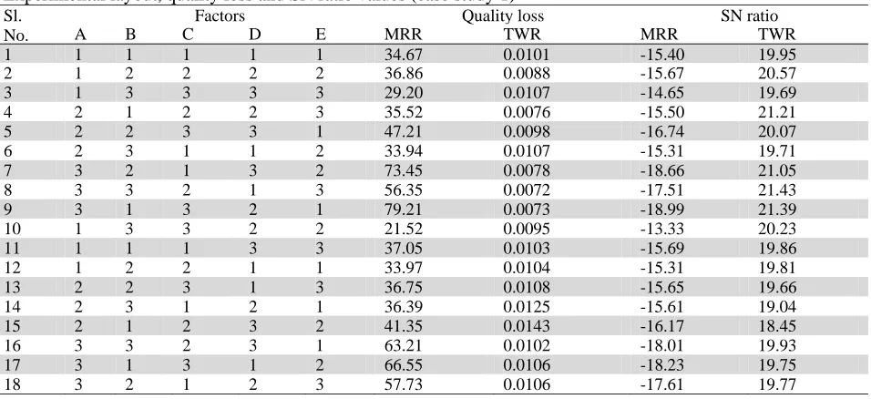
three levels for factor E (25, 50 and 75). Since they were interested to study the main effects only, they prepared the experimental layout using L18 orthogonal array. The experimental layout along with the quality losses and the SN ratio values for various responses as obtained from Kumar and Khamba’s (2010) experimental data are given in Table 1.
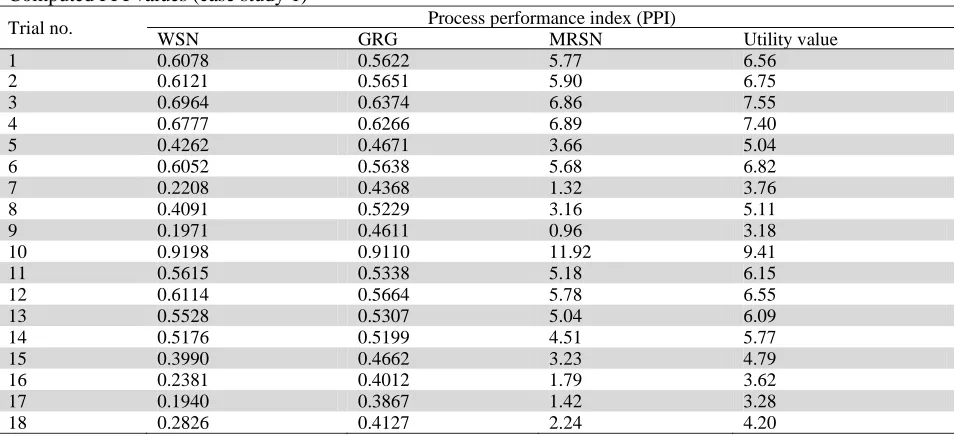
Often the relative importance of different responses is known to the process engineers. It can be observed from section 3 that all the four methods can take into account the relative importance of different responses by assignment of weights at some stages of computation of the PPI. According to Kumar and Khamba (2010) the weights for MRR and TWR should be 0.8 and 0.2 respectively. It is decided to apply all the four optimization methods assuming the same weighting scheme for MRR and TWR. The PPI values for WSN, GRA, MRSN and UT methods are computed using the steps as mentioned in sections 3.1, 3.2, 3.3 and 3.4.2 respectively. Table 2 shows the computed PPI values for the four multi-response optimization methods.
The level averages of the control factors on the PPI values of the four methods, i.e. WSN, GRG, MRSN and utility value are given in Table 3. It may be recalled from the discussion in section 3 that larger values of WSN, GRG, MRSN and utility value (bold faced) signify better quality. Consequently, the optimal conditions for the factors A, B, C, D and E with respect to WSN, GRG, MRSN and utility values are found to be A1B3C3D2E3,
2 2 3 3 1B C D E
A , A1B3C3D2E2and A1B3C3D2E3 respectively. It is interesting to note that both WSN and UT
methods result in the same optimal process condition. On the other hand, GRA and MRSN methods lead to the same optimal process condition.
Table 1
Experimental layout, quality loss and SN ratio values (case study 1)
Sl. No.
Factors Quality loss SN ratio
A B C D E MRR TWR MRR TWR
1 1 1 1 1 1 34.67 0.0101 -15.40 19.95
2 1 2 2 2 2 36.86 0.0088 -15.67 20.57
3 1 3 3 3 3 29.20 0.0107 -14.65 19.69
4 2 1 2 2 3 35.52 0.0076 -15.50 21.21
5 2 2 3 3 1 47.21 0.0098 -16.74 20.07
6 2 3 1 1 2 33.94 0.0107 -15.31 19.71
7 3 2 1 3 2 73.45 0.0078 -18.66 21.05
8 3 3 2 1 3 56.35 0.0072 -17.51 21.43
9 3 1 3 2 1 79.21 0.0073 -18.99 21.39
10 1 3 3 2 2 21.52 0.0095 -13.33 20.23
11 1 1 1 3 3 37.05 0.0103 -15.69 19.86
12 1 2 2 1 1 33.97 0.0104 -15.31 19.81
13 2 2 3 1 3 36.75 0.0108 -15.65 19.66
14 2 3 1 2 1 36.39 0.0125 -15.61 19.04
15 2 1 2 3 2 41.35 0.0143 -16.17 18.45
16 3 3 2 3 1 63.21 0.0102 -18.01 19.93
17 3 1 3 1 2 66.55 0.0106 -18.23 19.75
Table 2
Computed PPI values (case study 1)
Trial no. Process performance index (PPI)
WSN GRG MRSN Utility value
1 0.6078 0.5622 5.77 6.56
2 0.6121 0.5651 5.90 6.75
3 0.6964 0.6374 6.86 7.55
4 0.6777 0.6266 6.89 7.40
5 0.4262 0.4671 3.66 5.04
6 0.6052 0.5638 5.68 6.82
7 0.2208 0.4368 1.32 3.76
8 0.4091 0.5229 3.16 5.11
9 0.1971 0.4611 0.96 3.18
10 0.9198 0.9110 11.92 9.41
11 0.5615 0.5338 5.18 6.15
12 0.6114 0.5664 5.78 6.55
13 0.5528 0.5307 5.04 6.09
14 0.5176 0.5199 4.51 5.77
15 0.3990 0.4662 3.23 4.79
16 0.2381 0.4012 1.79 3.62
17 0.1940 0.3867 1.42 3.28
18 0.2826 0.4127 2.24 4.20
Table 3
Level averages on the WSN, GRG, MRSN and utility value (case study 1)
Factor WSN GRG MRSN Utility value
Level Level Level Level Level Level Level Level Level Level Level Level
A 0.668 0.530 0.257 0.629 0.529 0.437 6.90 4.83 1.82 7.16 5.99 3.86
B 0.440 0.451 0.564 0.506 0.496 0.593 3.91 3.99 5.65 5.23 5.40 6.38
C 0.466 0.491 0.498 0.505 0.525 0.566 4.12 4.46 4.98 5.54 5.70 5.76
D 0.497 0.534 0.424 0.522 0.583 0.490 4.48 5.40 3.67 5.74 6.12 5.15
E 0.433 0.492 0.530 0.496 0.555 0.544 3.74 4.91 4.90 5.12 5.80 6.09
The ultimate interest of an engineer is to minimise the overall quality loss, i.e. maximise the overall SN ratio value for his/her USM process. So the SN ratios of the individual responses under the optimal conditions with respect to different PPI values are predicted using the additive model (Phadke, 1989). Table 4 displays the predicted SN ratios for MRR and TWR under different optimal conditions. The results in Table 4 reveal that the optimal process condition derived based on the WSN or UT methods leads to higher total SN ratio value, i.e. better overall quality than what can be achieved under the optimal condition derived by the GRA or MRSN method.
Table 4
Predicted SN ratios under different optimal conditions (case study 1)
Optimization method Optimization
criteria Optimal condition
Predicted SN ratio
Total MRR TWR
WSN method WSN ratio A1B3C3D2E3 -13.89 dB 20.45 dB 6.56 dB
GRA method MRSN ratio A1B3C3D2E2 -14.01 dB 20.14 dB 6.13 dB
MRSN method GRG A1B3C3D2E2 -14.01 dB 20.14 dB 6.13 dB
UT method Utility value A1B3C3D2E3 -13.89 dB 20.45 dB 6.56 dB
4.2 Case study 2
effects of the control factors only. So they prepared the experimental layout using L18 orthogonal array. Kumar and Khamba (2008) determined the optimal machining conditions separately for MRR and SR using usual Taguchi method (Phadke, 1989) and found that the optimal process conditions for the two responses were different. The same experimental data of Kumar and Khamba (2008) are analyzed here using the considered four methods for the multi-response optimization.
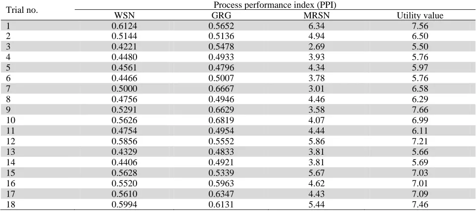
The experimental layout along with the quality losses and the SN ratio values for various responses as obtained from Kumar and Khamba’s (2008) experimental data are given in Table 5. Relative importance of MRR and SR are unknown. In the absence of any prior knowledge about the relative importance of the various responses, it is the most logical to assign the equal weights to all the responses. Therefore, all the methods are applied here considering that both MRR and SR are of equal importance, i.e. having equal weights. The PPI values for WSN, GRA, MRSN and UT approach are computed using the steps as mentioned in sections 3.1, 3.2, 3.3 and 3.4.2 respectively. Table 6 shows the computed PPI values for the four multi-response optimization methods.
Table 5
Experimental layout, quality loss and SN ratio values (case study 2) Sl.
No.
Factors Quality loss SN ratio
A B C D E MRR SR MRR TWR
1 1 1 1 1 1 32.22 0.325 -15.08 4.89
2 2 2 2 2 2 34.15 0.407 -15.33 3.90
3 3 3 3 3 3 24.75 0.733 -13.94 1.35
4 1 1 2 2 3 32.91 0.512 -15.17 2.91
5 2 2 3 3 1 41.25 0.400 -16.15 3.98
6 3 3 1 1 2 31.15 0.543 -14.93 2.65
7 1 2 1 3 2 84.96 0.172 -19.29 7.65
8 2 3 2 1 3 50.31 0.310 -17.02 5.09
9 3 1 3 2 1 76.63 0.175 -18.84 7.58
10 1 3 3 2 2 19.71 0.611 -12.95 2.14
11 2 1 1 3 3 35.34 0.441 -15.48 3.56
12 3 2 2 1 1 30.64 0.369 -14.86 4.33
13 1 2 3 1 3 34.38 0.512 -15.36 2.90
14 2 3 1 2 1 32.63 0.528 -15.14 2.78
15 3 1 2 3 2 38.78 0.312 -15.89 5.06
16 1 3 2 3 1 60.72 0.206 -17.83 6.86
17 2 1 3 1 2 64.92 0.188 -18.12 7.26
18 3 2 1 2 3 53.03 0.205 -17.25 6.87
Table 6
Computed PPI values (case study 2)
Trial no. Process performance index (PPI)
WSN GRG MRSN Utility value
1 0.6124 0.5652 6.34 7.56
2 0.5144 0.5136 4.94 6.50
3 0.4221 0.5478 2.69 5.50
4 0.4480 0.4933 3.93 5.76
5 0.4561 0.4796 4.34 5.97
6 0.4466 0.5007 3.78 5.76
7 0.5000 0.6667 3.01 6.58
8 0.4756 0.4946 4.46 6.29
9 0.5291 0.6629 3.58 7.66
10 0.5626 0.6819 4.07 6.99
11 0.4754 0.4954 4.44 6.11
12 0.5856 0.5552 5.86 7.21
13 0.4329 0.4833 3.81 5.66
14 0.4406 0.4921 3.81 5.69
15 0.5628 0.5339 5.67 7.03
16 0.5520 0.5963 4.62 7.01
17 0.5610 0.6347 4.43 7.09
The level averages of the control factors on the PPI values of the four methods, i.e. WSN, GRG, MRSN and utility value are given in Table 7. The larger values of WSN, GRG, MRSN and utility value (bold faced) signify better quality. Therefore, the optimal conditions for the factors A, B, C, D and E with respect to WSN, GRG, MRSN and utility values are chosen as A3B1C2D1E1, A1B1C3D2E2, A3B1C2D2E1and A3B1C2D1E1
respectively. It can be noted that both WSN and UT methods result in the same optimal process condition.
Table 7
Level averages on the WSN, GRG, MRSN and utility value (case study 2)
Factor WSN GRG MRSN Utility value
Level Level Level Level Level Level Level Level Level Level Level Level
A 0.518 0.487 0.524 0.581 0.518 0.569 4.30 4.40 4.50 6.59 6.28 6.77
B 0.531 0.515 0.483 0.564 0.552 0.552 4.73 4.57 3.91 6.87 6.56 6.21
C 0.512 0.523 0.494 0.556 0.531 0.582 4.47 4.92 3.82 6.53 6.63 6.48
D 0.519 0.516 0.495 0.539 0.576 0.553 4.30 4.78 4.13 6.68 6.60 6.37
E 0.529 0.525 0.476 0.559 0.589 0.521 4.76 4.32 4.13 6.85 6.66 6.13
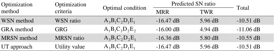
With the aim to compare the overall optimization performance of the four methods, the SN ratios of the individual responses under the optimal conditions with respect to different PPI values are predicted using the additive model (Phadke, 1989). Table 8 displays the predicted SN ratios for MRR and SR under different optimal conditions. The results in Table 8 reveal that the optimal process condition derived based on the WSN or UT methods leads to higher total SN ratio value, i.e. better overall quality than what can be achieved under the optimal conditions derived by the GRA and MRSN methods.
Table 8
Predicted SN ratios under different optimal conditions (case study 2) Optimization
method
Optimization
criteria Optimal condition
Predicted SN ratio
Total MRR TWR
WSN method WSN ratio A3B1C2D1E1 -16.47 dB 5.96 dB -10.51 dB
GRA method GRG A1B1C3D2E2 -16.00 dB 4.94 dB -11.06 dB
MRSN method MRSN ratio A3B1C2D2E1 -16.36 dB 5.80 dB -10.55 dB
UT approach Utility value A3B1C2D1E1 -16.47 dB 5.96 dB -10.51 dB
One limitation of the current research work is that there is no scope to carry out the confirmatory trial with any of the optimal factor-level combination. However, taking into consideration that the additive model for prediction is appropriate, which is usually true as highlighted by Phadke (1989) and Montgomery (1984), it can be said based on the above results that the WSN and UT method give better overall optimization performance than the GRA and MRSN methods for the multi-response optimization of USM process. However, WSN method is preferable to the UT method because its computational procedure is simpler. Therefore, it is recommended to use WSN method for simultaneous optimization of the multiple responses of USM process.
5. Conclusions
Ultrasonic machining (USM) process has multiple performance measures (responses), which are affected by several process parameters and the researchers commonly attempted to optimize USM process with respect to individual responses separately. In this paper, four relatively simple and easily comprehendible methods have been presented that can be effectively utilized for simultaneous optimization of the multiple responses of USM process and the overall optimization performances of the four methods have been compared. Based on the results the following conclusions are made:
a) The WSN or UT method, in general, gives better overall optimization performance for the USM process. b) However, WSN method is preferable to the UT method because it involve lesser computational
complexity.
References
Derringer, G., & Suich, R. (1980). Simultaneous optimization of several response variables.Journal of Quality
Dvivedi, A., & Kumar, P. (2007). Surface quality evaluation in ultrasonic drilling through the Taguchi technique.International Journal of Advanced Manufacturing Technology, 34, 131-140.
Gauri, S.K., Chakravorty, R., & Chakraborty, S. (2011). Optimization of correlated multiple responses of ultrasonic machining (USM) process.International Journal of Advanced Manufacturing Technology, 53, 1115-1127.
Hsi, H.M., Tsai, S.P., Wu, M.C., & Tzuang, C.K. (1999). A genetic algorithm for the optimal design of microwave filters.Intentional Journal of Industrial Engineering, 6, 282-288.
Hsieh, K.L., & Tong, L.I. (2001). Optimization of multiple quality responses involving qualitative and quantitative characteristics in IC manufacturing using neural networks.Computers in Industry, 46, 1-12. Jeyapaul, R., Shahabudeen, P., & Krishnaiah, K. (2005). Simultaneous optimization of multi-response problems
in the Taguchi method using genetic algorithm.International Journal of Advanced Manufacturing
Technology,30, 870-878.
Jadoun, R.S., Kumar, P. & Mishra, B.K. (2009). Taguchi’s optimization of process parameters for production accuracy in ultrasonic drilling of engineering ceramics.Production Engineering Research and Development, 3, 243-253.
Khuri, A.I. and Conlon, M. (1981) ‘Simultaneous optimization of multiple responses represented by polynomial regression functions’, Technometrics, Vol. 23, pp. 363-375.
Kumar, P., Barua, P.B., & Gaindhar, J.L. (2000). Quality optimization (multi-characteristics) through Taguchi technique and utility concept.Quality and Reliability Engineering International, 16, 475-485.
Kim, K., & Lin, D. (2000). Simultaneous optimization of multiple responses by maximizing exponential desirability functions.Journal of Royal Statistical Society: Series C (Applied Statistics), 43, 311-325.
Kumar, J.,& Khamba, J.S. (2008). An experimental study on ultrasonic machining of pure Titanium using designed experiments.Journal of Brazilian Society of Mechanical Science and Engineering, XXX, 231-238. Kumar, J., Khamba, J.S., & Mohapatra, S.K. (2008). An investigation into the machining characteristics of
titanium using ultrasonic machining.International Journal of Machining and Machinability of Materials, 3, 143-161.
Kumar, J., Khamba, J.S., & Mohapatra, S.K. (2009). Investigating and modelling tool-wear rate in the ultrasonic machining of titanium.International Journal of Advanced Manufacturing Technology, 41, 1107-1117.
Kumar, J., & Khamba, J.S. (2010). Modeling the material removal rate in ultrasonic machining of titanium using dimensional analysis.International Journal of Advanced Manufacturing Technology, 48, 103-119.
Montgomery, D.C. (1984).Design and Analysis of Experiments. New York: Wiley.
Phadke, M.S. (1989).Quality Engineering using Robust Design. New Jersey: Prentice Hall, Englewood Cliffs. Pignatiello, J.R., & Joseph, J. (1993). Strategies for robust multi-response quality engineering.Industrial
Engineering Research Division - IIE Transactions, 25, 5-15.
Ramakrishnan, R., & Karunamoorthy, L. (2006). Multi response optimization of wire EDM operations using robust design of experiments.International Journal of Advanced Manufacturing Technology, 29, 105-112. Rao, R.V., Pawar, P.J., & Davim, J.P. (2010). Parameter optimization of ultrasonic machining process using
non-traditional optimization algorithms.Materials and Manufacturing Processes, 25, 1120-1130.
Singh, P.N., Raghukandan, K., & Pai, B.C. (2004). Optimization by grey relational analysis of EDM parameters on machining Al-10%SiCP composites.Journal of Materials Processing Technology, 155-156, 1658-1661.
Singh, R., & Khamba, J.S. (2006). Ultrasonic machining of titanium and its alloys: A review.Journal of
Materials Processing Technology, 173, 125-135.
Singh, R., & Khamba, J.S. (2007). Taguchi technique for modelling material removal rate in ultrasonic machining of titanium.Material Science and Engineering, 460-461, 365-369.
Singh, R., & Khamba, J.S. (2009). Mathematical modeling of tool wear in ultrasonic machining of titanium.International Journal of Advanced Manufacturing Technology, 43, 573-580.
Tai, C.Y., Chen, T.S., & Wu, M.C. (1992). An enhanced Taguchi method for optimising SMT processes.Journal
of Electronics Manufacturing, 2, 91-100.
Thoe, T.B., Aspinwall, D.K., & Wise, M.L.H. (1998).Review on ultrasonic machining.International Journal of
Machine Tools and Manufacture, 38, 239-255.
Tong, L.I., & Hsieh, K.L. (2000). A novel means of applying artificial neural networks to optimize multi-response problem.Quality Engineering, 13, 11–18.
Tsui, K. (1999). Robust design optimization for multiple characteristic problems.International Journal of
Production Research,37, 433-445.