Virtual Engine – A Tool for a Powertrain Dynamic Solution

Virtual Engine - A Tool for a Powertrain Dynamic Solution

Pistek, V. ‒ Novotny, P. Vaclav Pistek* _{‒ Pavel Novotny}

Institute of Automotive Engineering, Faculty of Mechanical Engineering, Brno University of Technology, Czech Republic

The paper presents computational and experimental approaches to a powertrain vibration analysis. A complex computational model of a powertrain - a virtual engine is a powerful tool for a solution of structural, thermal and fatigue problems. The virtual engine results should answer different questions, mainly those concerning the area of noise, vibrations and component fatigues. The paper also includes a description of fast algorithm for a hydrodynamic solution of a slide bearing incorporating pin tilting influences. The main contribution is the fact that all models, that is those of a cranktrain, a valvetrain, a gear timing mechanism and a fuel injection pump are solved simultaneously, using a complex computational model. Synchronous solutions can have a fundamental effect on results of powertrain dynamics solutions. Additionally, it might help to understand influences among powertrain parts. The virtual engine is assembled as well as numerically solved in Multi Body System. Virtual engine results are validated by measurements on Diesel in-line six-cylinder engine.

© 2011 Journal of Mechanical Engineering. All rights reserved. Keywords: vibrations, noise, dynamics, powertrain, hydrodynamics

0 INTRODUCTION

Modern powertrains are complex thermo-mechanical systems improved by large and gradual development. Car producers still increase engine parameters like engine performance or torque together with a significant decrease of fuel consumption. Powertrains and cars supplied to European, US or Japanese markets have to be in compliance with national legislatives, which force the producers to significantly decrease noise, vibrations and emissions of every new powertrain. All these conditions have to be satisfied in very short developing periods.

Generally, the increase of engine performance often leads to an increase of powertrain noise and vibrations. Noise and vibration problems can be resolved by experimental or computational methods. Experimental methods are often very expensive which causes a fast development of modern computational methods. Modern computational methods can provide very exact results but only on condition that exact inputs are included. The inputs are often supplied by experimental methods. A portion of experimental methods continuously decreases, however, the experimental method still plays an important role in powertrain development.

All computational and measurement methods are applied to new turbocharged diesel inline six-cylinder engine. Some of the engine parameters are engine displacement 6.2 litres, peak power output 125 kW at engine speed 2200 rpm and compression ratio 17.8. The engine includes an OHV (Over Head Valve) valvetrain with two valves per cylinder and a camshaft located in a crankcase. The slide bearings are used for the bearing of the crankshaft as well as the camshaft. The valvetrain is driven by the front end of the crankshaft using helical gears. The engine incorporates a mechanically controlled fuel injection pump and other accessories like a piston compressor or an oil pump. The crankshaft includes a rubber torsional damper to decrease torsional vibrations. The design of the new engine originates from a turbocharged diesel inline four-cylinder engine.

1 THE STATE OF THE ART REVIEW

computational models being solved in time domain with high portions of flexible bodies. Other powertrain parts like a valvetrain, are included only as an additional mass or frequently, they are not included at all. Crankshaft and engine block interactions are solved using a hydrodynamics model of a slide bearing most often. A slide bearing model comes from a numerical solution of Reynolds equation, often without pin tilting influences [3] and [4] or with a simple pin tilting approximation [1]. Full elastohydrodynamic solution of Reynolds equation including shell and pin deformations is still not fully applied for powertrain dynamics with many slide bearings. The elastohydrodynamic solution of slide bearings of a separate connecting rod is often used for detailed slide bearing solutions. Theoretically, simultaneous full elastohydrodynamic solution of all cranktrain bearings can be used but numerical costs are high and there are no significant benefits for the cranktrain dynamics.

The present state of the art of rubber torsional damper computational models often includes a torsional spring and a torsional damper in a serial arrangement. This computational model does not describe rubber frequency behaviour for a solution in time domain correctly. For frequency dependencies it is necessary to use more complex models including Maxwell parts arranged in parallel. The rubber damper can sometimes influence axial crankshaft vibrations, therefore, axial properties have to also be incorporated Sometimes.

Valvetrain computational models have also been developed over a long period. First, discrete computational models of the valvetrain (still in use) included discrete point masses or springs. Springs have included only linear dependences of a force vs. a deformation. A tappet or a valve was excited by a lift function. With increasing Multi-Body Systems (MBS) the valvetrain computational models became more complex and incorporated rigid bodies and nonlinear contact forces. Later, some of the parts were replaced by spring-damper-mass bodies or beam bodies [6]. Camshaft angular irregularities on the basis of a separate cranktrain model solution were also incorporated. The present state of the art includes computational models with flexible parts. Spring models use flexible bodies with valve coil contacts enabling to understand

contacts between coils as well as spring stiffness changes [7] and [8]. The single valvetrain models are assembled to a complete valvetrain model [9]. However, drive timing mechanism or injection pump influences are not often included nor are influences of a compressor, an oil pump or other powertrain accessories.

So far each part of a powertrain has been solved separately. It has sometimes been extended by influences of other model results or measurement results but these results have been obtained from separate solutions. Valvetrain dynamic simulations can be taken as an example. A camshaft is driven by an angular velocity obtained from a separate cranktrain solution or from measurements. At present the need to solve all powertrain parts together continuously increases. This solution enables to include all interactions among parts. The results will show that, for example, valvetrain dynamics is highly influenced by a cranktrain but at the same time the cranktrain is slightly influenced by the valvetrain, both influenced by a timing drive or an injection pump.

2 COMPUTATIONAL METHODS 2.1 Virtual Engine

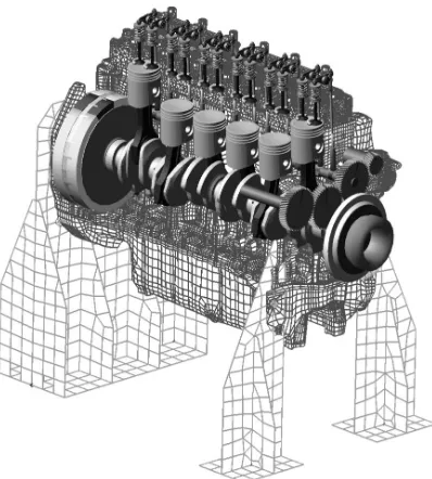
A complex computational model of the engine, in other words a virtual engine, is solved in time domain. This enables an incorporation of different physical problems including various nonlinearities. The virtual engine is assembled as well as numerically solved in MBS (Multi Body System) ADAMS.

ADAMS is a general code and enables an integration of user-defined models directly using ADAMS commands or using user written subroutines. The key features of the virtual model like the slide bearing model, the torsional damper model or gear timing drive model are incorporated into ADAMS model using Matlab program.

Fig. 1. Virtual engine including main subsystems

2.2 Flexible Parts

Flexible bodies represented by FE (Finite Element) models have a decisive importance on powertrain dynamics simulations. The FE models of each component should be created with special effort. In addition, a uniform FE mesh is often preferred.

In general, for a solution in time domain, FE models are very large and require a reduction. The discretization of a flexible component into a finite element model represents the infinite number of DOF (Degrees of Freedom) with a finite, but very large number of finite DOF. For the reduction of FE models, the Craig-Bampton method is used [10].

For the powertrain dynamic solution main components are treated as flexible models. A crankshaft model presents a fundamental component of the virtual engine. A reduced FE model is used for simulations of powertrain dynamics. The dynamics of powertrain moving parts are influenced by the stiffness of an engine block. Therefore, a reduced engine block FE model is also used for dynamics solutions. Reduced FE models of a camshaft, rockers and valve springs are used for a solution of valvetrain dynamics.

2.3 Torsional Rubber Damper Model

A torsional vibration damper is an important component of some cranktrains. It can significantly increase fatigue of engine parts together with a decrease of noise and vibrations. Different designs of torsional vibration dampers can be used. The rubber damper is chosen for the target engine.

Rubber mechanical properties can be characterized by very small compressibility and a high ability to reach large strains at small stresses without any plastic deformations. Maximal relative deformations of rubber can reach values of 800%. Force versus deformation rubber properties are strongly nonlinear. Therefore, Hook’s law cannot be used for stress-strain behaviour. Generally, every material is compressible, however, rubber can be treated as an uncompressible and isotropic material.

A phenomenological approach is used for the description of rubber mechanical properties. This approach does not originate from any molecular structure but comes from mathematical models. The Mooney-Rivlin two-parametric model is used for rubber structure modelling. This model introduces a hypothesis that strain energy W is a linear combination of two invariants of Finger tensor [11]:

W C I C I

d J

= ₁₀

(

₁−3

)

+ ₀₁

(

₂−3

)

+1

(

−1 ,

)

2 (1)

where I1 and I2 are the first and the second

invariant of a deviatoric component of Finger tensor, J is the determinant of a deformation gradient (for incompressible materials J = 1) and C10, C01 and d are constants. More information

about rubber material properties can be found in [11] and [12].

Pilot cranktrain dynamic calculations show that the loading frequency range is from 100 to 200 Hz.

The Mooney-Rivlin two-parametric model used for calculations is able to correctly describe rubber behaviour up to 30% of tension deformations and up to 10% of compression deformations. Real deformations in rubber damper are significantly smaller than these limit deformations. Mooney-Rivlin coefficients used for FE calculations and including temperature corrections are C10 = 1.065, C01 = 0.263 a d =

0.016.

A final rubber damper MBS model includes only global properties like torsional stiffness or axial stiffness.

A rubber damper MBS computational model has to incorporate dependency of torsional stiffness as well as torsional damping on frequency. FE solution founds the static torsional stiffness, the value is kT = 56145 Nm/rad and incorporates

no frequency dependencies. The frequency is incorporated using rubber frequency dependencies presented [11] and [12]. Torsional damping can be computed using frequency dependent torsional stiffness and relative damping as:

bT

( )

ω = kT( )_ωω χ, (2)

where kT(ω) is frequency dependent torsional

stiffness, χ is relative damping and ω is angular velocity.

Generally, the torsional damper can be described by parallelly arranged torsional stiffness and damper, however, the single arranged torsional stiffness and damping cannot be included as frequency dependent into MBS model.

Thus, a different approach has to be used for MBS simulations in time domain. A more complex MBS computational model of the torsional rubber damper has to be used. The model includes three serially connected Maxwell members (a spring and a damper). Two rigid parts (a damper ring and a damper flange) connected by a cylindrical joint and a serially arranged spring and damper in axial direction are also included in the model. The MBS model of the rubber damper is presented in Fig. 2.

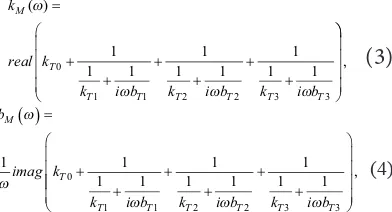
The torsional stiffness of the complex rubber model can be calculated using Eq. (3) and the torsional damping using Eq. (4).

k

real k

k i b k i b k i b

M

T

T T T T T T

( )ω

ω ω ω

=

+

+ + + + +



    

0

1 1 2 2 3 3

1

1 1 1 1 1 1 1 1



    

,

(3)

b

imag k

k i b k i b k i b

M

T

T T T T T T

ω

ω

ω ω ω

( )=

+

+ + + + +



  

1 1

1 1 1 1 1 1 1 1

0

1 1 2 2 3 3

 



    

, (4)

where kM is torsional stiffness of the torsional

damper, bM is torsional damping of the torsional

damper, kTi is torsional stiffness of i-spring, for

i=1,2,3 , bTi is torsional damping of i-damper and

kT0 is parallel torsional spring stiffness.

Fig. 2. MBS computational model of the torsional rubber damper

The resulted torsional stiffness kM and

damping bM are frequency dependent but each

spring or damper includes frequency independent values.

Fig. 3. Development process of MBS rubber damper computational model

Coefficients kTi, bTi a kT0 are found by

frequency range is chosen from 50 to 300 Hz and covers all significant frequencies occuring in the torsional damper.

The global stiffness values originate from a detailed solution of the three dimensional FE model in combinations with Matlab calculations. The development process starts with rubber shape and hardness proposals. The rubber hardness of 70 Shore is proposed from simple results of cranktrain torsional vibration calculations using a discrete torsional model. Fig. 3 shows the complete process of MBS rubber damper model development.

Generally, poor knowledge of rubber material properties is one of the main problems for a computational modelling of a cranktrain equipped with a rubber damper. The proposed approach for the determination of torsional damper global properties comes from elementary mechanical properties of rubber with a consideration of rubber frequency and temperature behaviour. However, this approach cannot produce highly accurate data because accurate rubber properties often do not exist. In addition, a rubber aging process or rubber producer tolerances (sometimes the rubber hardness tolerance is ±5 Shore) has to be also considered.

2.4 Slide Bearing Model Incorporating Pin Tilting Influences

Present computational models enable a description of a slide bearing behaviour in great detail. These models are often very complicated and require long solution times even on condition that only one slide bearing model is being solved. The target engine includes tens of slide bearings, therefore, all model features of slide bearings have to be carefully considered.

The loading capacity of a slide bearing model included in the virtual engine is considered in a radial direction and also incorporates pin tiltings, which means that radial forces and moments are included in the solution. For the solution of powertrain part dynamics elastic deformations can be neglected because integral values of pressure (forces and moments) for HD (hydrodynamic) and EHD (elastohydrodynamic) solution are approximately the same. This presumption is very important and it enables

a simplified solution. On the other hand, the solution can not be used for a detailed description of the slide bearing. Solutions of tens of EHD slide bearing models simultaneously seem to be extremely difficult and do not provide any fundamental benefits for general dynamics. The virtual engine therefore incorporates a compromise solution using the HD solution with elastic bearing shells and can be named (E)HD approach.

A HD approach presumes that shapes of a pin and a bearing shell are ideal cylindrical parts. The pin and the bearing shell are rigid bodies without any deformations. An oil gap between the pin and the shell is filled up but the oil and gap proportions are small in comparison with pin or bearing shell proportions. Only hydrodynamic frictions occur, while lubricating oil is incompressible and oil flow is laminar.

Generally, oil temperature has a significant influence on slide bearing behaviour. Oil temperature is treated as a constant for the whole oil film of the bearing. This presumption enables an inclusion of temperature influences after the hydrodynamic solution according to temperatures determined from similar engines.

In general, if the equation of the motion and the Continuity equation [2] are transformed for cylindrical forms of bearing oil gap together with restrictive conditions [2], the behaviour of oil pressure can be described by the Reynolds differential Eq. (5). This frequently used equation is derived for a bearing oil gap [1] or [2] and can be written in the form:

∂ ∂

∂ ∂  

 _ + _∂∂ _ ∂_∂ _ =  ∂_∂ + ∂_∂ 

 

  x h px z h pz U hx

h t

3 3 _{6η 2 , (5)}

where p is pressure, h is oil film gap, η is dynamic viscosity of oil and U is an effective velocity. The oil film gap is defined as:

h R r e= − + cos( ),ϕ (6) where R is a shell radius, r is a pin radius, e is a pin eccentricity and φ is an angle about pin axis.

The following relations can be defined as:

ϕ = x = R

x D

2 , Z Z

ψ = s = − ≅ − D

R r R

R r

r , ε = − e

R r, (7) where D is a shell diameter, B is a width of the bearing, Z is a dimensionless co-ordinate in the bearing axis direction, s is a bearing clearance, ψ is an independent bearing clearance and ε is dimensionless eccentricity.

A definition of a dimensionless oil film gap H in dependence on angle can be used:

H*_{( )ϕ ≅ +1 εcos .ϕ (8)}

Additionally, the pressures in oil film can be replaced by dimensionless pressures [5].

Π_D= pDψ

ηω

2

and

Π_{V =} pVψ

ηε

2



.

(9)

ΠD denotes dimensionless pressure

for a tangential movement of the pin, ΠV is

dimensionless pressure for a radial movement of the pin, ω is effective angular velocity and ε is a derivative of dimensionless eccentricity with respect of time.

Pin tilting angles can be introduced as:

γ γ

γ = tg

tg

*

max*

, (10)

δ δ

δ = tg tg

*

max*

, (11)

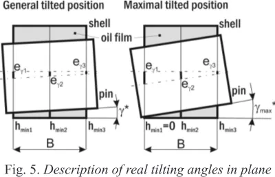
where γ is a dimensionless pin tilting angle in narrowest oil film gap and δ is a dimensionless tilting angle in the plane perpendicular to the plane of narrowest oil film gap. γ* _{denotes a real tilting}

angle in a plane of the narrowest oil film gap and γmax* denotes a maximal possible tilting angle in

the plane of the narrowest oil film gap for given eccentricity. δ* _{is a real tilting angle in the plane}

perpendicular to the plane of narrowest oil film gap and δmax* is a maximal real tilting angle in the

plane perpendicular to the plane of narrowest oil film gap for given eccentricity.

Fig. 4 presents the definition of pin tilting angles and Fig. 5 presents the definition of general and maximal tilting angle in a plane of the narrowest oil film gap.

Fig. 4. Definition of tilting angles of pin

Fig. 5. Description of real tilting angles in plane of the narrowest oil film gap

The final definition of the dimensionless oil film gap depending on tilting angles is:

H H

H Z Z

= =

= − −

( , , , )

( cos sin ),

*

ϕ ε γ δ

γ ϕ δ ϕ

1 (12)

and includes a dependency on two tilting angles. If the dimensionless oil film gap is used for the Reynolds equations for tangential and radial movements of the pin, then the Eq. (5) can be rewritten into two separate Eqs. [2] but with a modified definition of the dimensionless oil film gap.

∂ ∂

∂ ∂  

 



 + _∂∂  ∂_∂



 

  = ∂_∂

ϕ H ϕ ϕ

D

B Z H Z

H

D D

3 2

2 3 6

Π Π _{, (13)}

Likewise the dimensionless pressure is modified as follows [5]:

∂ ∂

∂ ∂  

 



 + _∂∂  ∂_∂



 _ =

ϕ H ϕ ϕ

D

B Z H Z

V V

3 2

2 3 12

Π Π

Π Π= H32_{. (15)}

If the Eqs. (10) to (12) are input into Eqs. (13) and (14), the final forms of Reynolds equations are:

∂ ∂ + 

 

 ∂_∂ + =

=

2 2

2 2 2

Π Π

Π

D D

D

D

D

B Z a Z

b Z

ϕ ϕ ε γ δ

ϕ ε γ δ

( , , , , )

( , , , , ),

(16)

∂

∂ +   

 ∂_∂ + =

=

2 2

2 2 2

Π Π

Π

V V

V

V

D

B Z a Z

b Z

ϕ ϕ ε γ δ

ϕ ε γ δ

( , , , , )

( , , , , ).

(17)

The equation term a(φ,ε,Z,γ,δ) is defined as:

a Z H HH H D

B Hz

( , , , , )ϕ ε γ δ = − _ϕϕ+ _ϕ+    _ 

  



  

−

3

4 2 2 2

2

2 _{, (18)}

and the equation terms bD(φ,ε,Z,γ,δ) and

bV(φ,ε,Z,γ,δ) are defined as:

bV( , , , , )ϕ ε Z γ δ = H Hϕ, − 6

3

2 ₍₁₉₎

bD( , , , , )ϕ ε Z γ δ = H cos .ϕ

−

12 32 ₍₂₀₎

Functions Hφ, HZ and Hφφ are partial

derivatives of the oil film gap and can be written as:

∂

∂ = + − −

− − =

H _{Z Z}

Z Z H

ϕ εγ ϕ γ ε ϕ

δ ϕ εδ ϕ _ϕ

sin ( )sin

cos cos ,

2

2

(21)

∂

∂ = − − −

− − =

H Z

H_Z

εγ ϕ γ ϕ

δ ϕ εδ ϕ

cos cos

sin sin ,

2

1

2 2

(22)

∂

∂ = + − +

+ + =

H

Z Z

Z Z H

ϕ

ϕϕ

ϕ εγ ϕ γ ε ϕ

δ ϕ εδ ϕ

2 2

2 2

cos ( )cos

sin sin , (23)

∂ ∂ = H

ZZ 0. (24)

Eqs. (16) and (17) are solved numerically. The FDM (Finite Difference Method) is used for a numeric solution.

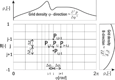
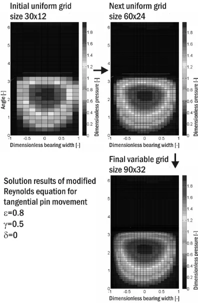
The FDM in basic form uses a constant integration step, however, this strategy can be disadvantageous because in casethe pin eccentricities are very high, the oil film pressure becomes concentrated in small areas so it is necessary to use a very small integration step. This leads to higher computational models. Therefore, FDM using variable integration step and multigrid strategies is developed.

The iterative solution starts using a very small computational grid. After a few iterations the results are approximated to a more dense grid and again a few iterations are solved. The new results are used for re-meshing the algorithm to generate new variable computational grid. The grid density is changed in dependency on the prescribed conditions (a pressure gradient). Three point integration scheme is chosen for the solution because for small integration steps it is very fast and the accuracy is similar to five-point integration scheme. Fig. 6 presents an example of computational grid for FDM with a variable integration step.

The resulted formula for iterative solution of dimensionless pressure at point i, j defines Eq. (29).

The formula for the numerical solution Eq. (29) is different for tangential and radial pin movement only in the term bD (for tangential pin

movement) and bV (for radial pin movement)

respectively.

Fig. 6. Computational grid for FDM with variable integration step

solution grid according to pressure differentiations with respect to the bearing angle and bearing width. This strategy enables solving problematic pressure zones in acceptable solution time.

Eq. (29) is solved iteratively for the tangential pin movement as well as for the radial pin movement. Initial and boundary conditions are the same for both solutions. The first boundary condition describes:

p

z=±B Z 



 _ ( =±)

= ⇒ =

2

1

0 Π 0. (25)

The only initial condition describes:

p(ϕ=0) = ⇒0 Π(ϕ=0) =0, (26)

This initial condition is used only for the first iteration and after that it is replaced by the cyclic boundary condition:

p_(ϕ=0) = p_{(ϕ π=2 )} ⇒Π_(ϕ=0)=Π_{(ϕ π=2 )}. (27)

The cavitation condition is included during the numerical solution. This condition resets negative pressures to zero values.

Eq. (33) describes real physical processes and does not allow negative pressures in liquids (a cavitation).

p= ∈ < ⇒0 p 0 Π= ∈ <0 Π 0. (28)

Fig. 7 presents solution results of modified Reynolds equation for tangential pin movement, relative eccentricity ε = 0.8, first pin tilting angle γ = 0.8 and second tilting angle δ = 0.

The computed pressure distributions have to be transferred to equivalent force systems for a solution in MBS. Pressure on an elementary surface can be imagined as an elementary force dF on this elementary surface dS. Integral values are dimensionless reaction forces F and reaction moments M and can be found by an integration of pressure across the whole bearing surface with coordinates φ and z.

Fig. 7. Solution results of modified Reynolds equation for tangential pin movement, relative eccentricity is ε = 0.8, first pin tilting angle is γ =

0.8 and second tilting angle is δ = 0

Elementary forces and moments for axes ”1“ and ”2“ can be defined as follows:

dF p dS

dF p dS

dF p dS

D D D D V V

1 2 1

= − = − = −

cos ,

sin ,

cos ,

ϕ

ϕ

(30)

dM p z dS

dM p z dS

dM p z dS

D D D D V V

1 2 1

= − = − = −

cos ,

sin ,

cos .

ϕ

ϕ

(31)

Π

∆ Π ∆ Π

∆ ∆

∆ Π

i j

i i j i i j j j

j i j

D V

D B

Z

,

, , ,

, =

+

+ +

+

+

− −

−

+

1 1

2

1 1

1

1 1

1

2 2

1

ϕ ϕ

ϕ ϕ

∆∆ Π

∆ ∆

∆ ∆ ∆ ∆

Z

Z Z b

D

B Z Z a

j i j

j j D V

j j j j

− −

−

− −

+ −

+ −

1 1

1

1 2 2

1

2 2

, ,

.

ϕ ϕ

The indexes 1 and 2 represent projections to axes „1“, „2“, index D means results for a tangential pin movement and index V means results for a radial pin movement.

The pressure distribution for radial pin movement is symmetrical, therefore, the forces F2V and moments M2V equal zero.

If all integration conditions are satisfied, the axis force components „1“ and „2“ can be found using equations:

F p dS p Rd dz

DB _{d d}

D D S D B B D 1 0 2 2 2 2 ₄ = − = − = = −

∫∫

∫

∫

− cos cos cos ϕ ϕ ϕ ηω ψ ϕ ϕ π

Π ZZ DB D

0 2

1 1

2 ₄ 1

π ηω ψ

∫

∫

− = Φ , (32)

F p dS p Rd dz

DB _d V V S V B B V 1 0 2 2 2 2 ₄ = − = − = = −

∫∫

∫

∫

− cos cos cos ϕ ϕ ϕ ηε ψ ϕ ϕ π

 _{Π ddZ} DB

V 0

2

1 1

2 ₄ 1

π ηε ψ

∫

∫

− =  Φ , (33)

F p dS p Rd dz

DB _{d d}

D D S D B B D 2 0 2 2 2 2 ₄ = − = − = = −

∫∫

∫

∫

− sin sin sin ϕ ϕ ϕ ηω ψ ϕ ϕ π

Π ZZ DB _D

0 2

1 1

2 ₄ 2

π ηω ψ

∫

∫

− = Φ , (34)

and components of moments for axes „1“ and „2“ can be found as:

M p z dS p z Rd dz

DB _{Z d}

D D S D B B D 1 0 2 2 2 2 ₄ = − = − = −

∫∫

∫

∫

− cos cos cos ϕ ϕ ϕ ηω ψ ϕ π Π ϕϕ ηω ψ π

dZ DB _D

0 2

1 1

2 ₄ 1

∫

∫

−

= Θ ,

(35)

M p z dS p z Rd dz

DB _Z D D S D B B D 2 0 2 2 2 2 ₄ = − = − = = −

∫∫

∫

∫

− sin sin sin ϕ ϕ ϕ ηω ψ ϕ π

Π dd dZϕ ηω DB _D

ψ π 0 2 1 1

2 ₄ 2

∫

∫

−

= Θ ,

(36)

M p z dS p z Rd dz

DB _Z V V S V B B V 1 0 2 2 2 2 ₄ = − = − = = −

∫∫

∫

∫

− cos cos cos ϕ ϕ ϕ ηε ψ π  _{Π ϕϕ ϕ} ηε ψ π

d dZ DB _V

0 2

1 1

2 ₄ 1

∫

∫

−

=  Θ .

(37)

The equivalent force system including the resulted force and moment can also be replaced by the force acting on an arm ξ.

Hydrodynamic databases include integral values Φ1D, Φ2D, Φ1V, Θ1D, Θ2D, Θ1V for chosen

ratios D/B and pin tilting. The resulted forces and moments (F1D, F2D, F1V, M1D, M2D, M1V) inserted

into MBS can be obtained by an inclusion of bearing sizes, bearing clearances, dynamic viscosity and pin kinematic values.

3 POWERTRAIN DYNAMIC SOLUTION RESULTS

3.1 Cranktrain Dynamic Solution Results The determination of cranktrain torsional vibrations represents a fundamental step in powertrain development. Cranktrain torsional vibrations influence torsional vibrations of each powertrain rotating component. These vibrations can significantly influence forces in every single valvetrain or forces in a gear timing drive. Fatigue of powertrain components like a crankshaft or a camshaft is also affected. An experimental determination of torsional vibrations using, for example, laser vibration tools is an advance and it can help to validate computational models.

Laser Vibrometer Type 2523 and POLYTEC 4000 Series Laser Vibrometer are used for torsional vibration measurements. These experimental tools enable measurements of angular velocities of arbitrary rotating parts.

Fig. 8. Harmonic analysis of crankshaft pulley torsional vibrations of an inline six-cylinder

engine with rubber torsional damper (a computation and a measurement)

Comparisons of computed and measured results show some differences. These differences are partially caused by different combustion pressures. The inline diesel four-cylinder engine was used for combustion pressure indications but these pressures are slightly different from the inline diesel six-cylinder engine used for torsional vibration measurements.

3.2 Valvetrain Dynamic Solution Results

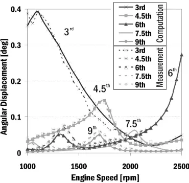
The camshaft vibrations are influenced mainly by cranktrain torsional vibrations and also by all single valvetrain torques, a gear timing mechanism and an injection pump torque. Fig. 9 presents harmonic analyses of measured and computed angular velocities of a camshaft end near to the camshaft bearing No. 1. There are mainly harmonic orders known from cranktrain torsional vibrations.

The results which can be very efficiently used for valvetrain computational model

validations are strains and stresses in some component parts. In the case of the target engine, strain gauge measurements on a rocker and an outer valve spring have been used. Relative strains and stresses from the same places respectively are analysed by computational models of a rocker and a spring.

Fig. 9. Harmonic order analysis of camshaft end angular displacement (a computation and a

measurement)

Fig. 10. Computed and measured stresses of the first cylinder intake rocker for engine speed 2200

rpm

cause inaccuracies in results. Valve spring stress measurements can be taken as an example. The calibration test deforms the valve spring in the form of the first mode shape (static shape) but in reality higher mode shapes can also be excited. They cannot be found by strain gauge measurements because they can lie on vibration nodes. Therefore, the calibrated force does not show any additional force.

Fig. 11. Computed and measured stresses of the first cylinder inline valve spring for engine speed

2200 rpm

The comparison of computed and measured stresses on a rocker surface in a given direction for an engine speed 2200 rpm is presented in Fig. 10. Fig. 11 shows a comparison of computed and measured stresses on an outer valve spring surface in a given direction for an engine speed 2200 rpm.

3.3 Powertrain Surface Velocity Solution Results

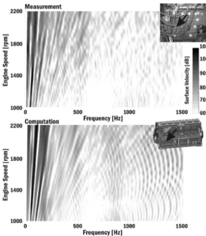
In general, powertrain surface vibrations and radiated noise are coupled. The noise produced by a powertrain can be understood from crankcase surface velocities. Fig. 12 shows measured and calculated Campbell diagrams of crankcase surface velocities near the second cylinder and crankshaft axis. The value 5.10-8 _ms-1 _{is used as}

a reference velocity. The measured results have been determined by POLYTEC Vibrometer OFV-5000.

The main area of the most significant velocity amplitudes is from 50 to 350 Hz. The first and second torsional frequencies (210 and 255 Hz) can be found in computed and in measured results. Engine attachments to the ground have a fundamental influence on surface velocities with frequencies up to 150 Hz. The computed and measured results show the movement of the whole engine (a rotation about a crankshaft axis direction) at natural frequency 66 Hz. The Campbell diagrams (Fig. 12) shows a resonance of this frequency at the engine speed 1300 rpm.

Fig. 12. Measured and calculated Campbell diagrams of crankcase surface velocities near the

second cylinder and crankshaft axis

4 CONCLUSION

subsystems. A detailed analysis of a connecting rod using thermo-elastohydrodynamic (TEHD) models of the slide bearings can be taken as an example.

The solution of powertrain part dynamics: The crankshaft, the camshaft or other component vibrations can be partially solved using independent models, however, the complex computational models provide more accurate results. What is more, they help to understand interactions between powertrain subsystems.

The solution of powertrain noise, vibrations and harshness: The complex computational models of the powertrain incorporating the most significant powertrain subsystems have to be used. Engine block models using reduced FE bodies should include all parts like covers, caps and intake or exhaust manifolds. All significant noise sources like combustion pressure forces, meshing gear forces or injection pump torques have to also be included into the powertrain model.

The virtual engine results can help to understand the NVH behaviour of a new powertrain and enable to speed-up the development process together with reductions of expensive prototypes. The presented computational approach enables an analysis the NVH properties of a powertrain in the range of days. The contribution of different modifications on existing virtual engine (different crankshaft design, added ribs on a crankcase etc.) can be found in range of hours or days.

Therefore, the computational tools based on FEM, MBS, EHD or CFD principles together with experimental tests play an important role in modern powertrain design.

5 ACKNOWLEDGEMENTS

The above activities have been supported by the grant provided by the GAČR (Grant Agency of the Czech Republic) reg. No. 101/09/1225, named “Interaction of elastic structures through thin layers of viscoelastic fluid«. The authors would like to thank GAČR for the rendered assistance.

6 REFERENCES

[1] Rebbert, M. (2003). Simulation der Kurbewellendynamik unter Berücksichtigung

der hydrodynamischen Lagerung zur Lösung motorakusticher Fragen. Ph.D. dissertation, Rheinisch-Westfälischen Technischen Hochschule, Aachen.

[2] Butenschön, H.J. (1976). Das hydrodynamische, zylindrische Gleitlager endlicher Breite unter instationärer Belastung. Ph.D. dissertation, Universität Karlsruhe, Karlsruhe.

[3] Knoll, G., Schönen, R., Wilhelm, K. (2006). Full dynamic analysis of crankshaft and engine block with special respect to elastohydrodynamic bearing coupling. Universität Gesamthochschule, Kassel. [4] Du, I. (1999). Simulation of flexible rotating

crankshaft with flexible engine block and hydrodynamic bearing for a V6 engine. Noise and Vibration Conference, Michigan, p. 89-96.

[5] Kuchař, P. (2007). Strength solution of dynamically loaded parts of combustion engines. Ph.D. dissertation. Prague.

[6] Strowe, Ch., Chattenberg, S. (2008). Friction and CO2 reduction through an integrated

approach of valvetrain components. ATZ Technology, vol. 8, no. 7, p. 256-261.

[7] Ortmann, Ch., Skovbjerg, H. (2000). ADAMS/Engine powered by FEV, Part 1: Valve Spring. International ADAMS Users Conference, p. 117-128.

[8] Du, I., Chen, J. (2000). Dynamic analysis of a 3D finger follower valve train system with flexible camshafts. SAE World Congress, p. 250-263.

[9] Knoll, G., Brands, Ch., Schönen, R. (2003). Elastohydrodynamic interaction of camshaft and bearings under consideration of valve train forces. MTZ Motortechnische Zeitschrift, vol. 64, no. 9, p. 724-734.

[10] Craig, R.R. (1981). Structural Dynamics. John Willey & Sons, New York.

[11] Paulstra, L. (2007). Modelling of automotive antivibration rubber parts. Fall 172nd

Technical Meeting of the Rubber Division of the American Chemical Society, p. 523-530. [12] Macosko, C.W. (1994). Rheology: principles,