University of New Orleans University of New Orleans
ScholarWorks@UNO
ScholarWorks@UNO
University of New Orleans Theses and
Dissertations Dissertations and Theses
Spring 5-18-2012
Pattern Recognition of Power System Voltage Stability using
Pattern Recognition of Power System Voltage Stability using
Statistical and Algorithmic Methods
Statistical and Algorithmic Methods
Varun Togiti [email protected]
Follow this and additional works at: https://scholarworks.uno.edu/td
Part of the Power and Energy Commons
Recommended Citation Recommended Citation
Togiti, Varun, "Pattern Recognition of Power System Voltage Stability using Statistical and Algorithmic Methods" (2012). University of New Orleans Theses and Dissertations. 1488.
https://scholarworks.uno.edu/td/1488
This Thesis is protected by copyright and/or related rights. It has been brought to you by ScholarWorks@UNO with permission from the rights-holder(s). You are free to use this Thesis in any way that is permitted by the copyright and related rights legislation that applies to your use. For other uses you need to obtain permission from the rights-holder(s) directly, unless additional rights are indicated by a Creative Commons license in the record and/or on the work itself.
Pattern Recognition of Power System Voltage Stability using Statistical and Algorithmic Methods
A Thesis
Submitted to Graduate Faculty of the University of New Orleans in partial fulfillment of the requirements for the degree of
Master of Science
In
Engineering
Electrical
By
Varun Kumar Togiti
B. E. Osmania University, 2009
ii
iii
Acknowledgement
I would like to express my deepest gratitude to my academic and research advisor, Dr. Parviz Rastgoufard for his guidance and constant support in helping me to conduct and complete this work. His firm grasps and forte on all diverse areas of power systems ensured a steady stream of ideas and inspired me in every stage of this work. He has been a great source of inspiration and I am his student forever.
I would also like to express my appreciation to the members of my committee Dr. Ittiphong Leevongwat, and Dr. Dimitrios Charalampidis for all their support and useful
feedback during my research. I would like to thank Entergy-UNO Power and Energy Research Laboratory for providing appropriate tools to finish this task.
I specially thank Nagendrakumar Beeravolu, for his valuable ideas and continuous guidance throughout this work.
iv
Table of Contents
List of Figures ... vii
List of Tables ... viii
Abstract ... ix
1 Introduction ... 1
1.1 Modern Power Systems ... 1
1.2 Power System Stability ... 2
1.3 Voltage Stability of Power System ... 3
1.4 A Review on Voltage Stability Analysis... 6
1.5 Pattern Recognition ... 10
1.6 A Review on Pattern Recognition in Power Systems ... 13
1.7 Historical Review on Major Blackouts ... 15
1.8 Scope of Work ... 17
2 Mathematical Modeling ... 19
2.1 Power System Stability ... 19
2.2 Rotor Angle Stability ... 19
2.2.1 Transient Stability Analysis ... 22
2.2.2 Equal – area criterion ... 24
2.2.3 Numerical Integration Techniques ... 26
2.2.4 Direct Method of Transient Stability Analysis – Transient Energy Function Approach ... 27
2.3 Voltage Stability ... 29
2.4 Voltage Stability Analysis ... 32
2.4.1 Dynamic Analysis ... 33
2.4.2 Static Analysis ... 34
v
2.4.4 Q-V modal analysis... 36
2.5 Pattern Recognition ... 37
2.5.1 Regularized Least Squares classification (RLSC) ... 37
2.5.2 Data Mining – Classification and Regression Trees (CART) ... 39
3 Power System Models for Simulation ... 43
3.1 Introduction ... 43
3.2 Power System Simulator for Engineering (PSSE) ... 43
3.2.1 Generator Model ... 44
3.2.2 Excitation System Model ... 47
3.2.3 Maximum Excitation Limiter Model ... 48
3.2.4 Turbine Governor System Model ... 49
3.2.5 Power System Stabilizer Model ... 50
4 Test System... 52
4.1 IEEE 39 Bus System ... 52
4.2 Bus Data ... 53
4.3 Generation Data... 54
4.4 Load Data ... 55
4.5 Branch and Transformer data ... 56
4.6 Excitation System and Maximum Excitation Limiter data ... 58
4.7 Turbine Governor Model data ... 59
5 Research Simulations and Results ... 60
5.1 Simulations in PSS®E ... 60
5.2 Regularized Least Squares Method ... 65
5.3 CART ... 65
vi
5.3.2 Feature 2... 67
5.3.3 Feature 3... 68
5.3.4 CART TREES ... 68
6 Summary and Future Work ... 71
6.1 Summary ... 71
6.2 Future Work ... 72
Bibliography ... 73
vii
L
IST OFF
IGURESSimple power system model ... 20
Power - angle curve ... 21
Single - machine infinite bus system ... 22
Equivalent Circuit ... 23
Response to a step change in mechanical power input ... 24
A ball rolling on the inner surface of a bowl ... 27
Region of stability and its local approximation ... 28
A simple radial system for illustration of voltage stability phenomenon ... 30
Receiving end voltage, current and power as a function of load demand ... 31
The - characteristics of the system of Figure 2.8 ... 32
characteristics of the system of Figure 2.8 with ... 33
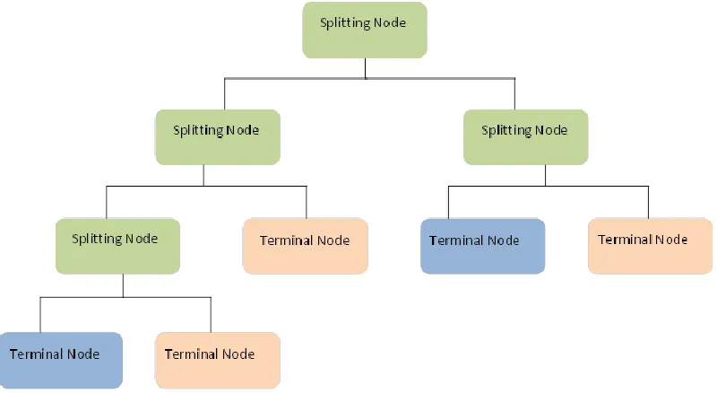
Classification Trees - After a successive sample partitions a classification decision is made at the terminal nodes ... 40
Generator model equivalent current source and Norton Equivalent Circuit ... 44
Electromagnetic Model of Round Rotor Generator (GENROU) ... 46
Rotating DC Exciter ... 47
ESDC1A excitation system model... 47
Inverse Time characteristics of MAXEX1 ... 48
Block Diagram of MAXEX1 ... 49
IEEG3 hydro governor model. ... 50
PSS2A Stabilizer Model ... 51
One line diagram of IEEE 39 bus system ... 52
Area chosen for voltage stability analysis ... 61
Voltage magnitude of Training case 3 - stable ... 63
Voltage magnitude of Training Case 12 – Unstable ... 64
Feature 1... 66
Feature 2... 67
viii
L
IST OFT
ABLESTable 2-1 Learning sample matrix with n attributes and m measurement vectors ... 40
Table 3-1 Reactances and Time Constants used for modeling ... 45
Table 4-1 IEEE 39 Bus, bus data ... 53
Table 4-2 IEEE 39 Bus, Generation data ... 54
Table 4-3 Generator Dynamics data ... 55
Table 4-4 IEEE 39 Bus, Load data ... 55
Table 4-5 IEEE 39 Bus, Branch data ... 56
Table 4-6 IEEE 39 Bus, Transformer data ... 57
Table 4-7 Excitation System data ... 58
Table 4-8 Maximum Excitation Limiter Model data ... 58
Table 4-9 Turbine Governor Model data ... 59
Table 4-10 Turbine Governor Model data (2) ... 59
Table 5-1 Training cases ... 62
Table 5-2 Testing cases ... 64
Table 5-3 Results from RLSC algorithm ... 65
Table 5-4 Feature 1 and data input format to CART ... 66
Table 5-5 Data format for feature 2 ... 67
Table 5-6 Data input format for feature 3 ... 68
Table 5-7 Data input format for CART ... 68
Table 5-8 CART output for testing cases ... 69
ix
A
BSTRACTIn recent years, power demands around the world and particularly in North America increased rapidly due to increase in customer’s demand, while the development in transmission
system is rather slow. This stresses the present transmission system and voltage stability becomes an important issue in this regard. Pattern recognition in conjunction with voltage stability analysis could be an effective tool to solve this problem
In this thesis, a methodology to detect the voltage stability ahead of time is presented. Dynamic simulation software PSS/E is used to simulate voltage stable and unstable cases, these cases are used to train and test the pattern recognition algorithms. Statistical and algorithmic pattern recognition methods are used. The proposed method is tested on IEEE 39 bus system. Finally, the pattern recognition models to predict the voltage stability of the system are developed.
1
Chapter 1
1
I
NTRODUCTIONThe purpose of this introductory chapter is to provide a general description of modern power systems, its stability and voltage stability in particular. Different kinds of pattern recognition techniques currently used are presented, particularly focusing on statistical and algorithmic approaches. A historical review of the voltage stability problem and the pattern recognition methods is presented. Finally, the outline of this thesis is explained.
1.1 MODERN POWER SYSTEMS
The commercial use of electricity began in the late 1870s when arc lamps were used for lighthouse illumination and street lighting [1]. The first complete electric power system (comprising of generator, cable, fuse, meter, and loads) was built by Thomas Edison- the historic Pearl Street Station in New York City which began operation in September 1882. With development of motors by Frank Sprague in 1884, motor loads were added to the systems.
These initial systems were dc (direct current). Eventually, ac (alternating current) systems dominated the dc systems for the following reasons:
Voltage levels can be easily transformed in ac systems.
AC generators are much simpler than dc generators.
AC motors are much simpler and cheaper than dc motors.
In early period of ac power transmission, frequency was not standardized. In order to facilitate the interconnection of different grids, 60 Hz was adopted as standard.
2
Interconnection of neighboring utilities usually leads to improved system security and economy of operation. Almost all the utilities in the United States and Canada are now part of one interconnected system. This results in a very large system of enormous complexity. The design of such a system and its secure operation are indeed challenging problems.
In recent years, power demands around the world generally and particularly in North America will experience rapid increases due to the increase of customers’ requirements. The report from Renewable Energy Transmission Company (RETCO) [2] about the infrastructure situation of U.S. electric grids states that electricity consumption accounts for 40% of all energy consumed in the U.S. and the electricity demand grows significantly and it will reach an increase rate of 26% by 2030.
Since 1982, growth in peak demand for electricity has exceeded transmission growth by almost 25% every year. Yet spending on research and development is the lowest of all industries [3]. Even with increase in demand, there has been chronic underinvestment in getting energy where it needs to go through transmission and distribution which limits grid efficiency and reliability. Since 2000, only 668 additional miles of interstate transmission have been built [3]. As a result, system constraints worsen at a time when outages and power quality issues are estimated to cost American business more than $100 billion on average each year. Under these extreme conditions, the need for maintaining stable operation of the grid is most important.
1.2 POWER SYSTEM STABILITY
“Power system stability is the ability of an electric power system, for a given initial
operating condition, to regain a state of operating equilibrium after being subjected to a physical disturbance, with most system variables bounded so that practically the entire system remains intact” [4]. This definition applies to an interconnected power system as a whole. The stability of a particular generator or a group of generators is of interest. A remote generator may lose synchronism without causing cascading instability of the whole system. Similarly, stability of particular loads or load areas may be of interest.
3
occurred. Power systems are subjected to a wide range of disturbances, small and large. Small disturbances such as changes in residential loads occur continuously; the system must be able to withstand these disturbances and operate in equilibrium condition. Large disturbances such as a short circuit on a transmission line or loss of a large generating unit may also occur. These disturbances may change topology of the system due to the isolation of faulted elements.
The power system in general is not designed to withstand all possible large disturbances possible because it is impractical and uneconomical [4]. The disturbances which have high probability of occurrence are chose while designing a contingency to study its mitigating process. A stable equilibrium set thus has a finite region of attraction; the larger the region, the more robust the system with respect to large disturbances.
Power system stability is a single problem; but in order to deal with different types of instabilities occurring in the system and study them effectively, we cannot treat it such. Because of high dimensionality and complexity of stability problem, it helps to make simplifying assumptions to analyze specific types of problems using an appropriate degree of detail of system representation and appropriate analytical techniques. The understanding of stability problems is greatly facilitated by the classification of stability into various categories [1]. The power system stability is mainly divided into rotor angle stability, frequency stability and voltage stability. Voltage stability problem is explained in detail as it is the main focus of this thesis.
1.3 VOLTAGE STABILITY OF POWER SYSTEM
4
The voltage instability is mainly caused because of the loads; after a disturbance, power consumed by the loads tends to be restored by the action of voltage regulators, tap changing transformers, and thermostats. Restored loads increase the stress on high voltage network by increasing the reactive power consumption and causing further voltage reduction. A run-down situation causing voltage instability occurs when load dynamics attempt to restore power consumption beyond the capability of transmission network and the connected generation [1], [5].
There is also a risk of overvoltage instability in the system which has been experienced at least once [6]. This is caused by the capacitive behavior of the network as well as by under excitation limiters preventing generators and/or synchronous compensators from absorbing the excess reactive power. This instability is associated with instability of the combined generation and transmission system to operate below some load level.
Voltage stability problems may also be experienced at HVDC links [7]. They are usually associated with HVDC links connected to weak ac systems and may occur at rectifier or inverter stations, and are associated with the unfavorable reactive power “load” characteristics of the converters. The HVDC link control strategies have a significant influence on such problems, since the active and reactive power at the ac/dc junction are determined by the controls. If the resulting loading on the ac transmission stresses it beyond its capability, voltage instability occurs. Such a phenomenon is relatively with the time frame of interest being in order of one second or less.
It is useful to classify voltage stability into sub categories as discussed below:
5
extend from a few seconds to tens of minutes. Therefore, long-term dynamic simulations are required for analysis
Small – disturbance voltage stability is the ability of the power system to maintain steady
permissible voltages when subjected to small perturbations such as incremental changes in system load. This form of stability is influenced by the characteristics of the load, continuous controls, and discrete controls at a given instant of time. This concept is useful in determining, at any instant, how the system responds to small system changes. To identify the factors influencing stability, system equations can be linearized for the analysis with appropriate assumptions.
The time frame of interest for voltage stability problems may vary from a few seconds to tens of minutes. Therefore, voltage stability can be classified into short term and long term on this basis.
Short – term voltage stability involves dynamics of fast acting load components such as induction motors, electronically controlled loads, and HVDC converters. The study period of interest is in order of several seconds, and the analysis requires solution of appropriate system differential equations [4]. This analysis needs dynamic modeling of loads.
Long – term voltage stability involves slower acting equipment such as tap-changing
6
1.4 AREVIEW ON VOLTAGE STABILITY ANALYSIS
Voltage stability problems mainly occur when the system is heavily stressed beyond its capability. While the disturbance leading to voltage collapse may be initiated by a variety of causes, the main problem is the inherent weakness in the power system. The main factors other than strength of transmission network, power transfer capability are generator reactive power/voltage control limits, load characteristics, characteristics of reactive compensation devices, and the action of voltage control devices such as under load tap changing transformers (ULTCs) [1].
The voltage stability analysis for a given system state involves the examination of two concepts [9]:
a) Proximity to voltage instability: A measure of how close the system is to voltage
instability? Physical quantities such as load levels, active power flow through critical interface and reactive power reserve can be used to measure the distance to instability. The most appropriate measure for a given situation depends on the specific system and the intended use of the margin. Considerations must be given to possible contingencies such as line outages, loss of generating units or reactive power sources, etc.
b) Mechanism of voltage instability: This includes the determination of the cause of
instability including the key factors, voltage - weak areas and also finding out the measures to improve stability.
7
The system dynamics influencing voltage instability are usually slow. Therefore, static methods can be used to analyze many aspects of the problem. The static analysis techniques allow examination of a wide range of system conditions and, if appropriately used, can provide much insight into the nature of the problem and identify the key contributing factors.
The electric utility has been largely dependent on conventional power-flow programs for static analysis of voltage stability. Stability is determined by generating V-P and Q-V curves at selected load buses. These curves are generated by executing a large number of power flows which is usually time consuming. These procedures focus on individual buses, that is, the stability is studied by stressing a particular bus in the system. This may unrealistically distort the stability of the system.
F. D. Galiana used load flow feasibility to indicate proximity to voltage collapse [10]. The feasibility region (FR) is defined as the set of generalized bus injections (P, Q, or V2 at each bus) for which a load flow exists. The feasibility margin is a scalar ranging between 0 and 1 which measures the proximity of a bus injection vector to the boundary of FR. This method does not rely on the load flow or optimal load flow simulations. Feasibility limit is to be defined from experience and then by monitoring a distance measure form this limit, one can monitor the voltage collapse condition.
V-Q sensitivity analysis has advantage that it provides voltage stability-related information from a system-wide perspective and clearly identifies areas that have potential problems [1].This method uses the conventional linearized power flow model. The elements of the Jacobian matrix give the sensitivity between power flow and bus voltage changes. The Jacobian matrix is reduced in size by considering P (real power) to be constant at each operating point. The V-Q sensitivity at a bus represents the slope of the Q-V curve at the given operating point. A positive V-Q sensitivity is indicative of stable operation; the smaller the sensitivity, the more stable the system. As stability decreases, the magnitude of sensitivity increases, becoming infinity at the stability limit. A negative sensitivity is indicative of unstable operation. A very small negative value indicates a very unstable operation.
8
smallest eigen values of a reduced Jacobian matrix (considering voltage and reactive power), and the associated bus, branch and generation participation factors. Each eigen value corresponds to a mode of voltage/reactive power variation and gives information about that mode. The small eigen values represent the modes most prone to loss of stability. The magnitude of each small eigen value provides a relative measure of proximity to loss of voltage stability for that mode. Bus, branch and generator participation factors provide useful information regarding the mechanism of loss of stability. This gives an insight of the system and helps in taking remedial actions to prevent the voltage collapse.
The load flow Jacobian and its properties are used to study the voltage instability [11] [12] [13]. The relationship between multiple load flow solutions and voltage instability has been studied by Y. Tamura, ET. Al. [11]. Under heavy – conditions, multiple load flow solutions are likely to appear. The authors suggest analyzing static and/or semi – dynamic performance of the problem and then the relationship between the dynamic factors and voltage instability. They assume that one is stable and the other is unstable if there is a pair of multiple load flow solution. Then a sequence of criteria is applied to the individual members of the solution pair to see their difference in behavior. Three criteria are used, the sign of Jacobian determinant in the load flow calculations, load flow sensitivity for load injections and system parameters, and stored energy of the elements L and C in the electric power system. For a stable operating condition, the sign of determinant of the Jacobian matrix is determined. Then as the system operating condition changes, for each condition, the sign of the determinant of the Jacobian is compared with the one determined earlier (for stable operating point). If the signs are equal, the system is assumed to be stable, if not unstable. This method has some uncertainty and this cannot be used as a standalone representation of instability. This method when used in conjunction with the other two criteria discussed above, can be used to determine the instability in power systems.
9
– Jun Cai, and Istvan Erlich proposed a novel approach which includes all possible active and
reactive power controls based on the multi-input multi-output transfer (MIMO) function and singular value decomposition (SVD) [14]. As seen in the above discussed approaches, the classical methods consider the active powers at all buses as constant. Voltage stability control methods such as reactive power compensation, under voltage load shedding, and transformer tap changers can also be taken into consideration using this method. These controls are selected as inputs to the MIMO system. The incremental changes in the bus voltage magnitudes are considered as the output variables. The input singular vectors are used to select the most suitable control signal for the improvement of steady state voltage stability and the output singular vectors provide an overview of the most critical buses that are affected by the static voltage stability. Since the inputs and outputs of the real system can be restricted to a small range, this method can also be applied to large power system networks.
Though static voltage stability analysis is used extensively in the power industry, there are some restrictions on this approach. The classic methods are mostly based on modal analysis, which requires the number of inputs (reactive power changes) be equal to the number of outputs (voltage magnitude changes). In large power systems, there may be additional controls which need to be included in the input. Only the effect of PQ-bus reactive power is considered, while in practice, the active power changes also have great influence on the static voltage stability. The effect of automatic voltage regulators (AVRs) cannot be included in the classic analysis [14].
Dynamic simulation accurately includes the time dependent actions of control and protection. Modeling for dynamics include more detailed representation of loads and all other equipment in power systems. Enormous increase in computing capacity has enabled us to use the dynamic simulations to analyze voltage stability problem. It still is a time consuming process, but a compromise between accuracy and speed by using other techniques is the fast dynamics [15]. A review on use of dynamic simulations for voltage stability analysis is presented below.
10
mid-term and long-term, the dynamics of slow acting devices such as transformer on-load tap changers (OLTC), generator over excitation limiters (OXL), etc., comes into play. Differential equations are used describe the dynamics of generators, OLTCs, OXLs, and loads. The effect of slow acting devices on long-term voltage stability is studied using MATLAB/SIMULINK.
J. H. Chow and A. Gebreselassie used eigen value analysis, sensitivity analysis, and nonlinear voltage simulations to study the dynamic phenomenon of voltage instability [17]. They analyzed a simple power system consisting of a single machine and a constant power load. Eigen value analysis approach is used to evaluate the effects of some of the control parameters on the voltage stability limits of the single machine system model. The eigenvalue analysis predicts the values of the system parameters for which, any small disturbance will initiate unstable voltage oscillations. ACSL (Advanced Continuous Simulation Language) is used to perform nonlinear simulation for the predicted system conditions and to investigate the effects of these oscillations. They have also determined the need for more detailed load, generation models to establish realistic stability properties.
M. Hasani and M. Parniani studied the voltage stability analysis using a method combining static and dynamic analysis [18]. Using static methods, a voltage stability ranking was performed to define faint buses, generators and links in terms of voltage stability. More detailed modeling was used to analyze the dynamics of most severe conditions. Many detailed dynamic analyses are done using more detailed modeling of loads and other equipment in power systems [19], [20]. T. X. Zhu, S. K. Tso, and K. L. Lo have investigated the effect of on-load tap changers on the maximum power transfer limit [21].
1.5 PATTERN RECOGNITION
11
computer vision, artificial intelligence, and remote sensing. This technique is being implemented in power systems field to develop tools which can take decisions automatically regarding various issues [23], [24,24], [25].
A pattern could be a fingerprint image, a handwritten cursive word, a human face or a speech signal. Given a pattern, its recognition/classification may consist of one of the following two tasks: 1) supervised classification in which the pattern is identified as a member of predefined class, 2) unsupervised classification in which the pattern is assigned to a hitherto unknown class. Here the recognition problem is posed as a classification or categorization task, where the classes are defined by the system designer (in supervised classification) or are learned based on the similarity of patterns (in unsupervised classification).
The rapid development of computing power, which enables fast processing of huge data sets, has also facilitated the use of elaborate and diverse methods of classification. The data being collected in every field is enormously increasing, such as P.M.U (Phasor Measurement Unit) data in the power industry. This creates a demand for automatic pattern recognition systems and also stringent performance requirements (speed, accuracy, and cost). In this development of process, no single recognition technique is “optimal”, so multiple methods and
approaches have to be used.
The design of pattern recognition system essentially involves the following three aspects: 1) data acquisition and preprocessing, 2) data representation (features), and 3) decision making. Learning from a set of examples (training set) is an important and desired attribute of most pattern recognition techniques. Various types of pattern recognition techniques are discussed below:
Statistical Approach: In statistical approach, each pattern is represented in terms of d
12
different classes. A disadvantage of this approach is that too much statistical information or unavailable statistical information may be needed for the solution.
Syntactic Approach: In this approach, a pattern is viewed as being composed of simple
subpatterns which are yet themselves built from yet simpler subpatterns [22]. The simplest/elementary subpatterns to be recognized are called primitives and the given complex pattern is represented in terms of the interrelationships between these primitives. In syntactic pattern recognition, a formal analogy is drawn between the structure of patterns and the syntax of a language. The patterns are viewed as sentences belonging to a language, primitives are viewed as the alphabets of the language, and the sentences are generated according to a grammar. Thus a large number of complex patterns can be described by a small number of primitives and grammatical rules. The grammar for each pattern class must be inferred from the available training samples. The implementation of this technique leads to difficulties which primarily have to do with the segmentation of noisy pattern (to detect the primitives) and the interference of the grammar from training set.
Neural Networks: Neural networks can be viewed as massively parallel computing systems consisting of an extremely large number of simple processors with many interconnections. Neural network models attempt to use some organizational principles (such as learning, generalization, and computation) in a network of weighted graphs in which the nodes are artificial neurons and directed edges (with weights) are connections between neuron outputs and inputs. The main characteristics of neural networks are that they have ability to learn complex nonlinear input – output relationships, use sequential training procedures, and adapt themselves to the data. A main disadvantage of the neural network approach is that it may take considerable computer time and memory. Another disadvantage is that we may not have enough representative training samples that would allow the solution to provide the necessary generalization to non-training patterns.
13
1.6 AREVIEW ON PATTERN RECOGNITION IN POWER SYSTEMS
Pattern recognition is being widely used in several fields of engineering and sciences including power systems. There have been many literatures on the use of pattern recognition for transient, dynamic stability assessment, controlled islanding, and many other applications in power systems, [23] , [24], [25].
L. S. Moulin, et al., applied support vector machines (SVM), a recently introduced learning – based nonlinear classifier approach to analyze transient stability analysis (TSA) in power systems [24]. Power systems analysis is enormously high dimensional problem, and this makes pattern recognition technique a promising tool for the analysis. The integration of automatic learning/pattern recognition techniques with analytical TSA methods can provide more accurate monitoring, fast decision making, etc.,. It also avoids the repetitive burden of analyzing similar operating points. Neural networks (NNs) technology has been reported as an important contributor for reaching the goals of online TSA [26]. Support vector machines (SVM) rely on support vectors (SVs) to identify the decision boundaries between different classes. SVMs can map complex nonlinear input/output relationships, and are well suited for TSA because our focus is on the boundary between stable and unstable operating points. Instead of using entire data available, features are extracted from it, and are used for pattern recognition. Feature selection reduces the input dimensionality in order to use as few variables as possible, getting a more concise representation of power system.
14
number of stable and unstable cases. The active and reactive power at the relevant buses is chose for training and the classifier is either stable (+1) or unstable (-1). The following conclusions are drawn [24]:
SVMs fit the TSA task for large power systems
SVMs performed better when complete data set was used (which include more stable
cases)
There have been some false dismissals (unstable cases classified as stable, which is extremely undesirable)
The stability studies database already available at the utilities can be used with NN-based
TSA.
A hybrid approach based on direct-type methods coupled with detailed time simulation is considered as a promising idea for TSA of large – scale power systems. The NNs can be used as filters to discard stable contingencies in a very fast way [27].
Peng Zhang and Jing Peng have studied the performance of support vector machines (SVMs) and regularized least squares (RLS) by applying both the techniques to a collection of data sets [28]. As discussed earlier, SVMs realize the structure risk minimization principle by maximizing the margin between the separating plane and the data. The regularized least squares (RLS) method constructs classifiers by minimizing a regularized functional directly in a reproducing kernel Hilbert space. The SVM solution produces a hyper plane having the maximum margin between different classes of data. Regarding complexity of solution, the computational cost associated with SVM is incurred by solving a quadratic programing problem. On the other hand, for RLS, linear system of equations is needed to be solved, which is less complex. Two methods are used with both real and simulated data. The performance of both methods is almost similar. The RLS methodology is strikingly simple. On the other hand, SVMs have a compact representation of solutions, which may be important in time – critical applications.
15
measurements and periodically updated decision trees (DTs) [29]. Phasor measurement units (PMUs) utilize the global positioning system (GPS) receivers and microprocessors to monitor the state of the power system; they are very accurate and fast. The time-stamped digital phasors calculated in the PMUs are synchronized to a common time frame by satellites and then assembled into a series of data streams for communication to remote control centers. The created database consists of different cases that are represented by a vector of predictors and an objective (for example secure or insecure state), a DT is designed for successful classification of this objective by using only a small number of these predictors. A number of pre-disturbance operating conditions (OC) for the past representative data and the forecasted ones for the next 24 hours are collected a day ahead. Detailed voltage security analysis is conducted for all these operating conditions for critical contingencies, and each contingency case at different OCs is then assigned a voltage security label. This can be either secure or insecure. By collecting PMU related system parameters, DTs are trained offline to obtain security classifications for next day. These DTs are updated on hourly basis, if there are any major changes in the system topology. The updated DTs are then used for online applications for next hour. Measurements from PMUs are continuously collected in real time and decision trees are used to assess the system condition. Decision trees can be combined with other data mining tools like support vector machine and random forests to pursue better prediction accuracy.
1.7 HISTORICAL REVIEW ON MAJOR BLACKOUTS
In the last decade, several major blackouts were reported in several research papers [31], [32], [33]. Deregulation was introduced to improve the managerial efficiency of power systems as its size and the load demand increased enormously. This created a competitive market structure, and increased the system utilization. This also increased the risk on system operations by stressing the power systems and reducing the predictability of operations [31]. Usually, a power system is designed for N-1 contingencies, but is still not enough to secure the system. The review of major blackouts will give the system designers an overview of the problems underneath and the mitigating steps to be taken in future.
16
southwest was the main cause. At heavy loading conditions, the backup protection tripped one out of five transmission lines. This is because the relay was set to low load level. Thus the other four lines were also successively tripped, diverting 1700 MW of power which overloaded several other lines and finally the system collapsed. It was identified that there was not enough spinning reserve at the time the blackout was initiated. Extra High Voltage transmission lines were proposed to be built, less essential load shedding was introduced, and keeping distributed spinning reserve was put into practice to avoid future collapses. This failure affected 30 million people; New York City was in darkness for 13 hours.
On 13th July 1977, there was a power failure due to the collapse of Con Edison system. The collapse resulted from a combination of natural events, equipment malfunctioning, questionable system design features and operating errors as lack of preparation for emergencies [34]. Severe thunderstorm and lightning strikes hit two lines; protective equipment of each line was imperfectly operated and resulted in three of the four lines tripping. Transmission ties increasingly overloaded for about 35 minutes and all ties were opened. After 6 minutes, the entire system was out of operation. This might have been easily prevented by a timely increasing of generation or manual load shedding. The system was instructed to operate well within the cautious interpretations of such severities. The research and development penetrated into the blackouts and more accurate modeling of the power system components was practiced.
A power failure occurred in Tokyo, Japan on 23rd July 1987 affecting 2.8 million customers with the outage of 3.4 GW power. The reserve was kept at 1.52 GW and it was sufficient to manage the usual demand increase. Unusual high peak demand due to extreme hot weather caused the failure. Increase in demand (400MW/minute) exceeded the expected level. This increasing demand gradually reduced the voltage of the 500 kV trunk network within 5 minutes to 460 kV. Constant power characteristic loads such as air conditioners reduced the network voltage rapidly and caused dynamic voltage instability. The system was recovered within 90 minutes. As future precautions, the operators increased the trunk line voltage by 5% of its normal operation during summer time. A 1 GW power plant was proposed to be built closer to the load center, and shunt capacitors together with SVC of 1,550 MVAR were installed.
17
power plants tripped. “Blackout was caused by deficiencies in specific practices, equipment, and human decisions by various organizations that affected conditions and outcomes that afternoon” [33]. The major reason was found to be insufficient reactive power, which leads to voltage instability. As the computer software systems were not operating properly, the operators were not warned in advance about the system condition. Failure initiated with a tripping voltage regulator due to over excitation and when the operators attempted to restore the regulators, generators tripped. These generators were generating high reactive power, which was continuously increasing as the day progressed. A 345 kV transmission line loaded with 44% tripped in 90 minutes due to tree contact. Another line loaded with 88% tripped at 128 minutes due to another tree touching. Finally critical failure made on a tie line 158 minutes later by a relay. The major tie line trip reversed the power flow and lead to cascading blackout of the entire region. The major tie line tripping might have been protected by load shedding.
According to the records of major disturbances, the system faults are cleared in milliseconds, then system fault transients remained for several seconds and blackouts occurred in several minutes. This show a scope, where if immediate actions were taken, the blackouts would have been prevented. Many research papers are being published on online voltage stability analysis techniques which could help prevent the blackouts.
1.8 SCOPE OF WORK
18
and also to preprocess the data which is to be analyzed with CART. This methodology could be a useful online application for voltage stability analysis in power systems.
19
Chapter 2
2
M
ATHEMATICALM
ODELINGMathematical modeling of the power system stability problem and voltage stability problem in detail are discussed in this chapter. Different methods to analyze the instability phenomena are explained.
2.1 POWER SYSTEM STABILITY
As mentioned in chapter 1, power system stability is the ability of power system to remain in state of operating equilibrium under normal operating conditions and to regain an acceptable state of equilibrium after being subjected to a disturbance. The stability analysis of power systems is broadly classified into two types:
Rotor Angle Stability
Voltage Stability
These two stability problems and their analyses are explained below:
2.2 ROTOR ANGLE STABILITY
Rotor angle stability is the ability of interconnected synchronous machines of a power system to remain in synchronism [1]. This stability problem involves electromechanical oscillations inherent to the power systems. The variation of electrical power output of synchronous machines with respect to the oscillations of the rotors is the main factor affecting stability.
20
A rotating magnetic field is created due to the alternating currents flowing in the armature winding. The stator and rotor fields interact with each other to produce an electromechanical torque. Under normal conditions, the stator and rotor fields rotate at the same speed, with an angular separation between them depending on the electrical power output of the generator.
The relation between transfer power and the angular positions of the rotors of the interconnected machines is an important factor in deciding stability. Let us consider a simple power system model shown in Figure 2.1. The figure represents a generator feeding a synchronous motor through a transmission line having inductance and negligible resistance and capacitance.
A simple model comprising of voltage behind an effective reactance is used to represent synchronous machines. The power transferred from the generator to the motor is a function of angular separation (δ) between the rotors of the two machines. The power transferred from generator to motor is given by
(2.1)
where
and
Figure 2.1 Simple power system model 𝑿𝑳
𝑿𝑮 𝑿𝑴
21
The power versus angle plot is shown in Figure 2.2. When the angle is zero, no power is transferred. As the angle increases, the power transferred increases up to a maximum. After a certain angle, nominally 90 , further increase in angle results in a decrease in power transferred. The magnitude of the maximum power transferred between two machines is directly proportional to the machine internal voltages and inversely proportional to the reactance between the voltages which include the reactance of the transmission line connecting the machines and the reactances of the machines. Stability is a condition of equilibrium between opposing forces in the power systems. Under normal operating conditions, there is equilibrium between the input mechanical and the output electrical torque of each machine and the speed remains constant. If the system is perturbed, this equilibrium is upset, resulting in acceleration or deceleration of the rotors of the generators according to the laws of motion. If one generator temporarily runs faster than the other, its angular position corresponding to the slower machine advances. The resulting angle transfers a part of load from slower machine to the faster machine as per the power – angle relationship. This tends to decrease the speed difference and thus the angular separation. If the angular separation increases beyond a certain limit, the power transfer decreases; which further increases the angular separation leading to instability.
In electric power systems, the change in electrical torque of a synchronous machine following a perturbation can be resolved into two components:
Figure 2.2 Power - angle curve
P
22
(2.2)
Where is the component of torque change in phase with the rotor angle perturbation
and is referred to as synchronizing torque coefficient. is the component of torque in
phase with the speed deviation and is referred to as damping torque component. Both synchronizing and damping torques are needed for stable operation of power systems. Lack of sufficient synchronizing torque results in instability through an aperiodic drift in rotor angle. On the other hand, lack of sufficient damping torque results in oscillatory instability.
The rotor angle stability is further categorized into small signal stability and transient stability.
Small signal stability is the ability of power system to maintain synchronism under small disturbances which occur continually because of variations in loads and generations. The instability may arise due to insufficient synchronizing or damping torques.
Transient stability is the ability of the power systems to maintain synchronism when
subjected to severe transient disturbances such as a fault on transmission facilities, loss of generation or loss of a large load, etc. Stability depends on both the initial operating state of the system and is influenced by the nonlinear power - angle relationship.
2.2.1 TRANSIENT STABILITY ANALYSIS
The nature of transient stability is explained here. In the system shown in Figure 2.3 [1], a generator is delivering power to a large system represented by an infinite bus through two transmission circuits. The system model is reduced to the form shown in Figure 2.4 .
Figure 2.3 Single - machine infinite bus system
Infinite Bus
𝑬𝒕 𝑿𝟏 𝑬𝑩
23
The generator’s electrical output is
(2.3)
The equation of motion or the swing equation can be written as
(2.4)
Where is the mechanical power input to the generator, H is the inertia constant, δ is the rotor angle and t is time in seconds.
The transient behavior of the system can be examined by considering a sudden increase in the mechanical input from to as shown in Figure 2.5 [1]. Because of inertia of the rotor, the rotor angle cannot change directly from to corresponding to the new equilibrium point b at which . As the mechanical power is more than the electrical output, the rotor accelerates from the initial point to the point tracing the curve according to the swing equation. At any instant, the difference between mechanical input and electrical output represents the accelerating power. When point is reached, the accelerating power is zero but the rotor speed is higher than the synchronous speed (corresponding to the infinite bus). Hence, the rotor angle continues to increase. For values of δ higher than , is greater than
and the rotor decelerates. At some peak value the rotor speed recovers to the synchronous value , but is higher than which causes the rotor to decelerate with the speed dropping
Figure 2.4 Equivalent Circuit 𝑬∠𝜹
𝑿𝑻
24
below the operating point retraces the curve from c to b and then to a. The rotor angle oscillates indefinitely about the new equilibrium angle . If we consider all the resistances and the complete model of generator, many positive damping forces act on the rotor causing it to reach the new equilibrium point b.
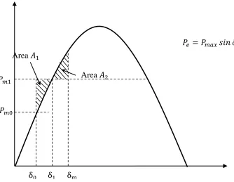
2.2.2 EQUAL – AREA CRITERION
It is not necessary to solve the swing equation to find out whether the rotor angle increases indefinitely or settles at equilibrium point for disturbances. Using the power angle diagram shown in Figure 2.5, stability limits can be calculated. Rearranging and integrating (2.4) gives
𝑃𝑚
Figure 2.5 Response to a step change in mechanical power input 𝑃𝑒 𝑃𝑚𝑎𝑥𝑠𝑖𝑛 𝛿
Area 𝐴
Area 𝐴
𝑃𝑚
25
[
] ∫
( )
(2.5)
The speed deviation
is initially zero. It will change as a disturbance occurs. For stable
operation, the deviation of angle δ must reach a maximum value and then change direction. This
requires becoming zero after disturbance. The criterion for stability can be written as:
∫ ( ) (2.6)
Where the initial rotor is angle and is the maximum rotor angle as shown in Figure 2.5. The area under the function plotted against δ must be zero if the system is to be stable. Kinetic energy is gained by the rotor during acceleration from to . The energy gained is
∫ ( ) (2.7)
The energy lost during deceleration when δ changes from to is
∫ ( )
(2.8)
The stability is maintained only if an area at least equal to can be located above
.The criterion for stability can be stated as follows:
26
2.2.3 NUMERICAL INTEGRATION TECHNIQUES
In time domain simulation, which is the most practical method of transient stability analysis [1], the nonlinear differential equations are solved by using step-by-step numerical integration techniques. Equations for generating units and other dynamic devices in the power systems can be expressed as follows:
̇ ( ) (2.9)
( ) (2.10)
where
state vector of individual device
R and I components of current injection from the device into the network
R and I components of bus voltage
The overall system equations, including the differential equations (2.9) for all the devices and combined algebraic equations for the devices and the network are expressed in the following general form comprising a set of first order differential equations
̇ ( ) (2.11)
and a set of algebraic equations
( ) (2.12)
with a set of known initial conditions ( ), where
state vector of the system
bus voltage vector
27
Depending on the modeling of the devices, and computational capabilities, several approaches are available to solve these equations. Numerical techniques most widely used are the Euler method, Modified Euler method and Runge-Kutta (R-K) methods [1]. These methods essentially utilize the Taylor series expansions to solve the equations.
2.2.4 DIRECT METHOD OF TRANSIENT STABILITY ANALYSIS – TRANSIENT ENERGY
FUNCTION APPROACH
The direct methods determine the stability without explicitly solving the system differential equations. The transient energy function approach and its application to the power systems stability is explained in detail.
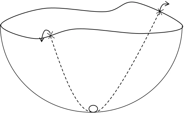
The transient energy approach can be described by considering a ball rolling on the inner surface of a bowl as shown in Figure 2.6 [1].
The area inside the bowl represents the stability region and the region outside is the region of instability. The rim has different heights at different points which represent different operating boundaries. Initially, the ball rests at the bottom of the bowl, this state is referred as stable equilibrium point (SEP). When the ball is injected by some kinetic energy, it moves in the direction determined by the applied energy. If the ball is able to convert all the kinetic energy into potential energy before crossing the boundary, then it rolls back to the SEP. If the kinetic energy applied is high enough to force the ball outside the rim, then the ball enters into the region of instability and it will never return to SEP. The surface inside the bowl represents the
28
potential energy surface and the rim of the bowl represents the potential energy boundary
surface (PEBS).
Application of this technique to power systems can be analyzed in a similar way. The system is initially at stable equilibrium point. If a fault occurs, the generators oscillate and the system gains kinetic and potential energy and moves away from the SEP. After fault clearing, the kinetic energy is converted into potential energy. To avoid instability, the system must be capable of absorbing the kinetic energy at a time when the forces are trying to bring the system back to equilibrium point. For a post disturbance condition, there is a maximum or critical amount of energy that the system can absorb. Assessment of transient stability requires functions that describe the transient energy responsible to separate one or more synchronous machines from the rest of the system and an estimate of critical energy required for the system to lose synchronism.
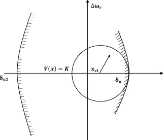
When a disturbance occurs, there is a stable equilibrium point for the post fault system. A region of attraction can be defined for this post fault SEP as shown in Figure 2.7 [1]. The post fault trajectory for which the state of system at fault clearing ( ) lies inside this region of
Figure 2.7 Region of stability and its local approximation
𝑽(𝒙) 𝑲
𝛚𝐫
𝛅𝐮𝟐
𝐱𝐜𝐥
29
attraction will eventually converge to the SEP, and the system is said to be stable. On the other hand, if lies outside the region of attraction, the post fault system will not converge to the stable equilibrium point and the system is said to be unstable.
The direct method solves the stability problem by comparing ( ) which is the value of energy function evaluated at to the critical energy . The system is stable if ( ) is less
than and the quantity ( ) is a good measure of system relative stability and is called transient energy margin.
As shown in Figure 2.7, if the rotor oscillates within the range and , the system will remain transiently stable and if the rotor swings beyond this limits, the system becomes unstable. These two points and form a boundary for stable oscillations and is called potential energy boundary surface (PEBS). The boundary of the stability region is approximated
locally by a constant energy surface { | ( ) } as shown in Figure 2.7, where represents the critical energy of the post fault system.
Application of the direct methods to power systems is limited to simple representation of generator and load models [1]. These methods are vulnerable to numerical problems while solving stressed systems. Heavy computational burden involved may increase the time taken to solve the problem, making it slower than time-domain simulations.
2.3 VOLTAGE STABILITY
30
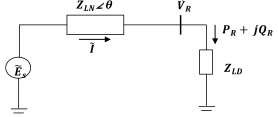
The voltage stability phenomenon can be examined by considering the relationships between the transmitted power ( ), receiving end voltage ( ), and the reactive power injection
( ). These characteristics are presented for the simple radial system shown in Figure 2.8.
The current I and receiving end voltage and power are given by the following equations:
√
(2.13)
√
(2.14)
(
)
(2.15)
Where
Figure 2.8 A simple radial system for illustration of voltage stability phenomenon
𝒁𝑳𝑵∠ 𝜽 𝑽𝑹
𝑷𝑹 𝒋𝑸𝑹
𝒁𝑳𝑫∠ 𝚽 𝑬𝒔
𝑰
𝐹 (𝑍𝐿𝐷
𝑍𝐿𝑁) (
𝑍𝐿𝐷
31
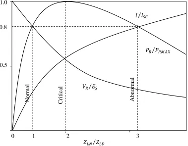
Figure 2.9 shows the plots of I, and as a function of load demand ⁄ for the case with and . As load demand increases, increases suddenly at first, slowly at the maximum value and then decreases. The values of and I corresponding to maximum power are referred to as critical values. For a given value of , there are two operating points corresponding to two different values of . This is shown in Figure 2.9
for . The point to the left corresponds to the normal operation. For the point to the right, I is much larger and is much smaller than the point to the left. This corresponds to the abnormal operation and is highly undesirable. For a load demand higher than the maximum power, control of power by varying load would be unstable. The increase in load admittance would decrease the power. The load characteristics and the action of voltage control devices have an adverse effect on the voltage and may cause it do decrease progressively. This phenomenon is called voltage instability.
1.0
0.8
𝑍𝐿𝑁⁄𝑍𝐿𝐷
Figure 2.9 Receiving end voltage, current and power as a function of load demand
Abnor
mal
C
ritica
l
Nor
mal
𝐼 𝐼⁄𝑆𝐶
𝑃𝑅⁄𝑃𝑅𝑀𝐴𝑋
𝑉𝑅⁄𝐸𝑆
32
2.4 VOLTAGE STABILITY ANALYSIS
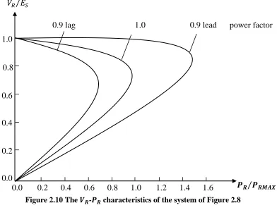
The V-P and Q-V characteristics have been most widely used for the voltage stability analysis. Figure 2.10 shows the relation between receiving end voltage and power for load
at different power factors These correspond to the simple radial system considered in Figure 2.8
[5]. These curves are produced by using a series of power flow solutions for different load levels. For each curve, the load in a certain area under consideration is uniformly scaled up while maintaining the power factor constant. At the “knee” of the V-P curve, the voltage drops rapidly
with increase in load demand. Power – flow solution fails to converge, which is indicative of instability. Operating the system at stability limits is unsecure and a satisfactory operating condition is ensured by allowing sufficient “power margin”.
Figure 2.10 The 𝑽𝑹-𝑷𝑹 characteristics of the system of Figure 2.8
0.0 0.2 0.4 0.6 0.8 1.0 1.2 1.4 1.6
0.9 lag 1.0 0.9 lead power factor
𝑉𝑅⁄𝐸𝑆
𝑷𝑹⁄𝑷𝑹𝑴𝑨𝑿
1.0
0.8
0.6
0.4
0.2
33
Voltage stability is affected considerably by the variations in Q (reactive power consumption) at the loads. A more useful characteristic for voltage stability analysis is the Q-V relationship, which shows the sensitivity of bus voltages with respect to reactive power injections and absorptions. The bottom of the Q-V curve, where the derivative ⁄ is equal to zero, represents the voltage stability limit. Operation on the right side of Q-V curve is stable and on the left side is unstable.
2.4.1 DYNAMIC ANALYSIS
As discussed previously (Section Transient Stability Analysis), dynamic analysis of power systems involve solution for first order differential equations, which can be expressed in the following general form:
Figure 2.11 𝑽𝑹−𝑸𝑹 characteristics of the system of Figure 2.8 with 𝑷𝑷𝑹
𝑹𝑴𝑨𝑿 𝟎 𝟓
𝑷𝑹
𝑷𝑹𝑴𝑨𝑿 𝟎 𝟓
𝑷𝑹𝑴𝑨𝑿 is the
maximum power at unity power factor
𝑄𝑅⁄𝑃𝑅𝑀𝐴𝑋
𝑽𝑹⁄𝑬𝑺
0.0 0.2 0.4 0.6 0.8 1.0 1.2 1.4 1.6
1.00
0.75
0.50
0.25
0.00
-0.25
34
̇ ( ) (2.16)
and a set of algebraic equations
( ) (2.17)
with a set of known initial conditions ( ), where
state vector of the system
bus voltage vector
current injection vector
network node admittance matrix
The representation of transformer tap-changers and phase-shift angle controls are also included in the model, due to which the elements of change as a function of bus voltage and time. The current injection vector I is a function of the system states and bus voltage vector V, representing the boundary conditions at the terminals of the various devices. Equations (2.16) and (2.17) can be solved in time-domain using numerical techniques and network power flow analysis methods. The study period is typically on the order of several minutes.
2.4.2 STATIC ANALYSIS
35
2.4.3 V-Q SENSITIVITY ANALYSIS
The network constraints represented by Equation (2.17) can be expressed in the following linearized form:
[ ] [
] [ ]
(2.18)
where
incremental change in bus real power
incremental change in bus reactive power injection
incremental change in bus voltage angle
incremental change in bus voltage magnitude
⁄
The elements of the Jacobian matrix give the sensitivity between power flow and bus voltage changes. System voltage stability is affected by both P and Q. In this analysis, at each operating point, P is kept constant and voltage stability is analyzed by considering the incremental relationship between Q and V. Based on these considerations, in Equation (2.18), let
Then
(2.19)
where
[ − ] (2.20)
and is the reduced Jacobian matrix of the system. From Equation (2.20), we can write
− (2.21)
36
increases. A negative sensitivity is indicative of unstable operation. A small negative sensitivity represents a very unstable operation.
2.4.4 Q-V MODAL ANALYSIS
Voltage stability characteristics of the system can be identified by computing eigenvalues and eigenvectors of the reduced Jacobian matrix defined by Equation (2.20). This matrix can be decomposed into left eigenvector, right eigenvector, and eigenvalue matrices as shown
(2.22)
where
Right eigenvector matrix of
Left eigenvector matrix of
Diagonal eigenvalue matrix of
Rearranging Equation (2.22) and substituting it in Equation (2.21) gives
∑ (2.23)
Where is the column right eigenvector and the row left eigenvector of . Each eigenvalue and the corresponding right and left eigenvectors and define the
mode of the Q-V response. The modal analysis is performed using the Equation (2.24).
where
is the vector of modal voltage variations
is the vector of modal reactive power variations
37
In Equation (2.24), − is a diagonal matrix and this equation represents uncoupled first order equations. For the mode we have
(2.25)
The stability criterion is formulated as follows. If , then the system is voltage stable. If , then the system is voltage unstable. The magnitude of determines the degree of stability of the modal voltage. The smaller the magnitude of positive , the closer the modal voltage to being unstable. When , modal voltage collapses because any change in that modal reactive power causes infinite change in the corresponding modal voltage.
2.5 PATTERN RECOGNITION
As discussed previously in section 1.5, “Pattern recognition is the study of how machines
can observe the environment, learn to distinguish patterns of interest from their background, and make sound and reasonable decisions about the categories of the pattern” [22]. The two methods
the author has used are Regularized Least Squares Classification (RLSC) and Classification and Regression Trees (CART). The detailed explanation of these methods is presented.
2.5.1 REGULARIZED LEAST SQUARES CLASSIFICATION (RLSC)
The basic idea of this algorithm is to fit the “training” set of data ( ) with a function with a closed subset of and that generalizes, or is predictive. This algorithm can be derived from Tikhonov regularization [36] .
We consider the data ( ) where takes values { }. The goal is to come up with a function ( ) while minimizing the probability of error described by Equation (2.26).
( ( ( ))) (2.26)
38
∑( ( ) )
(2.27)
which is in general ill-posed, depending on the choice of the hypothesis space . Following Tikhonov we minimize, instead, over the hypothesis space , for a fixed positive parameter γ, the regularized functional :
∑( ( ) )
‖ ‖
(2.28)
where ‖ ‖ is the norm in – the Reproducing Kernel Hilbert Space (RKHS), defined by the kernel .
The solution for Tikhonov regularization problem can be solved by Representer Theorem [37] and is:
( ) ∑ ( )
(2.29)
The solution is obtained as follows. First, the kernel matrix is constructed from the training set S.
( ) ( )
Next step is to compute the vector coefficients ( ) by solving the system of linear equations
( ) (2.30)
![Figure 3.2 Electromagnetic Model of Round Rotor Generator (GENROU) [39]](https://thumb-us.123doks.com/thumbv2/123dok_us/8941926.1851294/56.612.116.572.93.642/figure-electromagnetic-model-of-round-rotor-generator-genrou.webp)
![Figure 3.3 Rotating DC Exciter [39]](https://thumb-us.123doks.com/thumbv2/123dok_us/8941926.1851294/57.612.116.553.487.667/figure-rotating-dc-exciter.webp)