Volume 7 - Article 6 | Pages 307–342

(1)

in the population sciences published by the Max Planck Institute for Demographic Research Doberaner Strasse 114 · D-18057 Rostock · GERMANY www.demographic-research.org

DEMOGRAPHIC RESEARCH

VOLUME 7, ARTICLE 6, PAGES 307-342

PUBLISHED 08 AUGUST 2002

www.demographic-research.org/Volumes/Vol7/6/

DOI: 10.4054/DemRes.2002.7.6

Research Article

Childbirth in East and West German

Stepfamilies

Estimated probabilities from hazard rate models

Dr. Ursula Henz

(2)

1 Introduction 308

2 Analyses of stepfamily fertility 310

3 Model 312

3.1 Model specification 312

3.2 The probability of having another child 316

4 Data set and Variables 317

4.1 Data set 317

4.2 Identifying non-shared children 318

4.3 Some partnership characteristics 319

4.4 Covariates 321

5 Results from the multivariate models 323

6 Summary and Discussion 329

7 Acknowledgements 330

Notes 331

References 333

(3)

Research Article

Childbirth in East and West German Stepfamilies

Estimated probabilities from hazard rate models

Dr. Ursula Henz1

Summary

(4)

1. Introduction

The present paper discusses modelling issues concerning the comparison of childbearing behaviour of stepfamilies and families with no children from earlier partners. The predominantly methodological question is discussed using the example of East and West Germany.

In recent years the rise in the number of stepfamilies in most Western countries has increased the interest in this family form (Hobcraft and Kiernan 1995). In West Germany four percent of all children are stepchildren while this is true for ten percent of all children in East Germany (Bien, Hartl and Teubner 2001). Stepfamilies are often described as having special problems, resulting in a lower stability of stepfamilies compared to families without stepchildren (Friedl 1988, Ganong and Coleman 1994, Walper 1993).

The problems of stepfamilies result from a number of factors, for example from the multiple tensions experienced in stepfamilies, the special developmental tasks required in these families, and the lack of role definitions for parents and children in stepfamilies (Friedl 1988, Furstenberg 1987, Nave-Herz 1994, Walper 1993). One way of strengthening the cohesion of the new family is to have another child. The new child can bind all the different family members together and thereby counterbalance their disparate interests and needs. One could, therefore, assume a high probability for a first common child in stepfamilies.

Many couples do, however, abstain from having a common child. The parents may fear that a new child may cause additional tensions in the family. Furthermore, at least one partner in a stepfamily has experienced a family break-up and may be sceptical about having another child. Finally, financial considerations, or related considerations about housing or employment, may also deter the couple from having another child.

The present paper analyses stepfamily fertility in East and West Germany focusing on the impact of children from earlier partners. Fertility decisions in stepfamilies differ from the patterns observed for childless partnerships because the two partners have separate fertility histories and often are at different stages of the parenting processes. They may have a different number of children, children at very different ages, or one of them may not yet be a parent at all.

(5)

higher birth rate than couples with a shared child. According to the parenthood hypothesis one expects, ceteris paribus, a higher birth rate if one partner has not yet a child of his or her own compared to a situation where both partners are already parents. Couples have a second child to provide a sibling for the first child (sibling hypothesis). In stepfamilies any shared child of the couple has at least one half-sibling. Whether the half-sibling can fully take the role of an older sibling should depend on the frequency of contact between the children as well as on the age gap between them.

The main interest of the present paper is to obtain a valid model for comparing childbearing behaviour of stepfamilies and families with no children from earlier partners. It turns out that the ceteris-paribus conditions from the previous paragraph are difficult to translate into a statistical model. In a recent paper Thomson and colleagues characterised the situation of the couple by the total number of children of both partners, both partners’ ages, calendar time and duration since partnership formation or since the birth of the previous shared child (Thomson et al. in press). The present paper elaborates and modifies this analysis. One problem of comparing childbirth in stepfamilies with childbirth to partners with only shared children is caused by the genuine difference in the measure of time. While the risk for conception is assumed to start at union formation for couples without a shared child it starts at the birth of the previous shared child for couples who have already a shared child. The models assume proportional birth rates in the two situations. There is, however, no obvious argument why the two birth rates should be proportional. The assumption can be tested by giving up the proportionality assumption of birth rates for couples with and without a shared child. Instead separate baseline hazard rates are estimated for different patterns of parenthood. The estimation results show that the shape of the birth rates differ considerably between couples with and without a child from an earlier partnership.

The models presented in Thomson and colleagues’ paper (Thomson et al. in press) allow testing directly the hypotheses derived from the value-of-children approach. Giving up the proportionality assumption means that these hypotheses cannot be tested directly any more. Instead I suggest an indirect method for evaluating the hypotheses. The estimated model parameters are used to calculate estimated probabilities of childbirth for various durations and covariate combinations. These estimated probabilities can depict the differences between childbearing behaviour of families with and without children from earlier partnerships as they are predicted by the model.

(6)

section 3.2. The data set and the variables are described in section 4. Section 5 gives the results for the German data. Conclusions are presented in section 6.

2. Analyses of stepfamily fertility

Early studies of childbirth after remarriage have compared the average number of children of women in stable partnerships with that of women who had experienced a partnership breakdown.(Note 1) Divorced, widowed, and re-married women were found to have fewer children at the end of their fertile ages than women who stayed in their first marriages. To understand these differences one needs to consider further circumstances that typically differ between women in stable marriages and women who experience partnership disruption. Consequently, later analyses of stepfamily fertility have used multivariate models, i.e. hazard rate models.

Studying women’s fertility in a second marriage, Griffith, Koo and Suchindran (1985) estimated the effect of woman’s prior child bearing, controlling for a number of other indicators. Using the 1973 National Survey of Family Growth they found that birth rates were highest if the youngest child was below two years of age. “It appears that having a new child is an important part of the process of creating a new family and that many couples seek to begin this process quickly” (ibid. p. 82). Griffith, Koo and Suchindran did not find a significant impact of the woman’s number of children.

In another study of childbirth in women’s second marriages, Wineberg (1990) used the 1985 Current Population Survey. He found that women who had two or more children at remarriage had lower odds of having a child in the new marriage than women with zero or one child at remarriage. Wineberg interpreted this finding as support for the view that “a child is needed to confirm adult status and complete one’s family” (ibid. p 37).

Jeffries, Berrington and Diamond (2000) have presented a study of childbearing after marital dissolution using data about Britain. The analysed time period starts right at the end of women’s first marriage; that is both times in and outside of partnerships are included. The findings are similar to those of Griffith and colleagues. Women with a child under age five are more likely to have another baby, while parity at marital dissolution has only a small impact on the birth rate.

(7)

1997). The paper addresses fertility decisions of all married couples and considers information about both partners’ children from previous unions. In the 1987-88 interview of NSFH, both spouses give details about their children living in the household and, if appropriate, about their children living elsewhere. Thomson presents models for conception during the period from six month after the first interview until up to six months after the second interview in 1992-94. She estimates rates for various configurations of his children, her children, and shared children, finding support for the union-confirmation hypothesis, the parenthood hypothesis and the sibling hypothesis. Due to small numbers for some of the configurations, many differences are, however, not significant.(Note 2)

In another study, Vikat, Thomson and Hoem (1999) have analysed fertility patterns in Swedish stepfamilies. They have estimated hazard rate models for the first birth in the current union, for second and for third births in the current union, for lifetime first births and for lifetime second and third births. The results indicate that a couple wants a shared child independently of either partner’s parity at union formation. The study provides no support for the parenthood hypothesis, as there was no difference in the rate of first shared birth according to whether the respondent was childless or not.

Buber and Prskawetz (2000) estimated hazard-rate models for first births in second unions in Austria. They found support for the union-commitment hypothesis but no support for the parenthood hypothesis. Buber and Prskawetz distinguished between co-resident and non-co-resident children from earlier partnerships. In Austria, first-birth rates in a second union are predominantly influenced by children who live in the household while non-resident children have only a weak influence.

(8)

However, the direct comparison of couples with and couples without a shared child comes at a price. It consists of the difficulty of defining the start of the period when the couple is at risk of conceiving a child. Thomson and collaborators use the birth date of the previous shared child as the starting point if the couple already has a shared child. Otherwise, the date of partnership formation is used. Problems associated with this specification will be discussed further in section 3.1.

Another elaboration of stepfamily fertility models refers to the endogeneity of the number of children born in a stepfamily to the partnership process. Lower birth rates in stepfamilies may be related to the lower stability of this kind of partnerships. Thomson and collaborators (1999) have simultaneously estimated birth rates and several other events in the partnership history, namely union dissolution, transforming a cohabiting union into marriage, and whether the union was formed by cohabitation or by marriage. By introducing terms for unobserved heterogeneity it was possible to test to what degree selectivity processes have an impact on the estimated effect of pre-union parity on the birth rate. The results showed only weak effects of unobserved heterogeneity. The union commitment hypothesis of first births in stepfamilies is supported. Furthermore it was shown that the probability of childbirth is reduced if the youngest child is more than three years old.

3. Model

3.1 Model specification

The present paper investigates birth rates in partnerships with children. Time starts at union formation if the couple already has a child at this point in time, and it starts anew after each childbirth within the union. The start of the partnership is the date of moving together or the marriage date, whichever occurred first.

As pointed out before, the genuine difference in process time in studies of first births and higher order births in a union could be problematic. In the paper by Thomson and collaborators (in press), time starts at union formation for first births in a union and at the birth of the previous child for second and higher order union births. In both cases process time ends at conception, that is nine months before the birth, or, if the couple does not have another child, at partnership break-up or interview, whichever occurs first.(Note 3) If the rates of first and of higher order birth in a union are proportional, a common baseline can be assumed and differences in birth rates can be estimated by using appropriate covariates.

(9)

similar fertility processes. It assumes that the couples are in comparable stages of decision making about having a(nother) child, and especially that they plan similar moratoria of trying to conceive a(nother) child. These assumptions can be disputed. Moving together is for some couples the start of a period of togetherness that may or may not lead to shared children at a later stage. Other couples start living together with the explicit wish to form a family soon. In the latter case women are sometimes already pregnant when the couple moves together. This is not possible for fertility processes that start at childbirth.

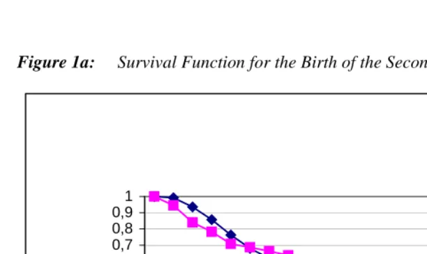
Figure 1a: Survival Function for the Birth of the Second Child; West-Germany

0 0,1 0,2 0,3 0,4 0,5 0,6 0,7 0,8 0,9 1

0 1 2 3 4 5 6 7 8

Years since begin of partnership or birth of first child Orthodox family

(10)

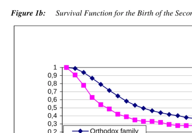
Figure 1b: Survival Function for the Birth of the Second Child; East-Germany

Figures 1a and 1b show survival functions for the birth of a second child for partnerships where the first child is a shared child or a non-shared child. For West Germany the second birth rates follow a specific pattern. Compared to orthodox families, stepfamilies have higher rates of having a second child during the first one and a half years. In the following three years, the birth rates are higher in orthodox families. In East Germany, stepfamilies have a considerably higher birth rate in the first two and a half years than orthodox families. By that time about 50 percent of all stepfamilies are estimated to have a second child compared to only 30 percent of all orthodox families. For longer durations the gap between childbirth probabilities in orthodox and in stepfamilies decreases.

The different patterns suggest that for some couples partnership formation may be endogenous to the fertility process. The data set does, however, not provide the dates when the couples began dating, which would otherwise allow a more appropriate measurement of process time. Therefore, process time is measured as described above. In the following the proportional hazard assumption for the two types of families is tested by estimating two alternative models: one model assuming proportionality and another model which allows for different baseline birth rates of couples with a shared child and for couples with only non-shared children. Especially for West-German men the numbers for some of these family types are rather small. As a result the estimated

0 0,1 0,2 0,3 0,4 0,5 0,6 0,7 0,8 0,9 1

0 1 2 3 4 5 6 7 8

Years since partnership formation or first child birth Orthodox family

(11)

parameters have high standard errors, but the substantial differences in the baseline rates make the model specification still worthwhile. In all models a piecewise-linear log-hazard rate is assumed (Lillard 1993). More precisely, the proportional hazard model can be written as

Ln λ ( t | x ) =

s

r

T ( t ) +

γ

r

X (1)

with

s

r

T ( t ) the baseline hazard and X the vector covariate values (Lillard and Panis

2000). The non-proportional hazard model can be written as

Ln λ ( t | x ) =

s

r

T ( t ) +

s

r

_AT ( t ) (No shared child = 1) +

γ

r

X. (2)

A more detailed formulation of the model can be found in section 4.4.

A drawback of the non-proportional model specification is that the differences between stepfamilies and orthodox families are no longer captured by one or two specific parameters. The non-proportional model does not provide a straightforward statistical test for the partnership and the parenthood hypotheses. It is, however, possible to compute the estimated probability of having another child within a certain time period based on the estimated model parameters. The probability associated with the different types of parenthood experience will be used for assessing the hypotheses derived from the value-of-children approach. Section 3.2 describes the calculation of the event probability for a piecewise-linear log-hazard rate model.

The consideration about endogeneity in section 2 could be implemented in the model by allowing for effects of unobserved heterogeneity. The study by Thomson et al. (1999) suggests that the effects are likely to be small. In addition, it is not desirable to further increase the complexity of the model because already now some estimates have very high standard errors due to the small number of observations in some groups.

Under standard assumptions the parameters in model (1) and model (2) are ordinary maximum likelihood estimators (Andersen et al. 1992). Especially, the

assumption of

s

r

_A=0 can be tested with the likelihood-ratio test. As four additional

(12)

3.2 The probability of having another child

The event probability can be calculated from the well-known relationship between the survivor probability S (t) and the hazard rate λ(t):

(

−

_∫

)

= t u du

t S 0 . ) ( exp )

( λ (3)

The model assumes that logλ is a linear spline. A linear spline function is a continuous function that is characterised by a pre-specified set of arguments, the so-called nodes, between which the function is linear with possibly varying slopes. Let 0=d0 < d1 < … <

dk-1 < dk = ∞ be the nodes. For each t ≥ 0 there is a node

d

l_twith

d

lt

≤

t

<

d

lt+1

.

For

slope parameters s0, s1, …sk-1 the log-hazard rate can be written as

∑

= +

−

+

=

lt

j

j j

j

d

t

d

s

y

t

0

1

0

*

(min(

,

)

).

)

(

log

λ

(4)

Let yl be the value of logλ at dl: y_l = log λ(d_l).Then the integrated hazard rate can

be written as

∫

t

u

du

=

t

u

du

0 0

))

(

log

(

exp

)

(

λ

(5)

∑ ∫

₌ + = lt

j t j d j d du u 0 ) , 1 min( )) ( log ( exp

λ

. )) ( * exp( 0 ) , 1 min(

∑ ∫

₌ + + −

= lt

j t j d j d j j

j s u d du

(13)

Applying elementary integration rules, (5) simplifies to

[

exp( *min( , )) exp( )

]

. * ) exp( ) ( 1 0 0 j j j j t l j j j j j t d s t d s s d s y du

u = − ₊ −

=

∑

∫

λ

(6)

The probability of having an event up to time t can then be written as

[

exp( *min( , )) exp( )

]

. * ) exp( exp 1 ) ( 1 ) ( ₁ 0         − − − − = − = ₊ =

∑

j j j j

t l j j j j j d s t d s s d s y t S t P (7)

Formula (7) can be used to calculate the estimated probability for an event up to time t for a certain covariate constellation. The nodes dj are known because they have been

fixed in advance. Estimates of the slope parameters sj are obtained directly from the

model output. The effects of covariates enter the estimated probability through the yj

-values. Constant covariates have only effects on y0. Formula (7) can be easily modified

to estimate probabilities for values of time-constant or time-varying covariates. In the model presented below with nodes at 1, 2 and 5 years the slope parameters for families with a shared child are s0, s1, s2 and s3. For families without a shared child they are

calculated as s0+ sA0, s1+ sA1, s2+ sA2 and s3+ sA3.

4. Data set and Variables

4.1 Data set

(14)

The German FFS sample consists of respondents aged 20 to 39 at the interview. This relatively young age is one of the reasons why a substantial number of respondents never had lived with a partner by the time of the interview, and only about 10 percent of the respondents had had more than one partner.(Note 5) For the analyses presented below all partnerships of a respondent are selected during the course of which the couple had at least one child, whether shared or non-shared.

The comparison of fertility decisions in stepfamilies and orthodox families is based on counting all biological children of both spouses towards the couple’s total parity. Variations in the birth rate are studied by different child configurations within the same total parity.(Note 6) Therefore, only periods in partnerships are selected when the couple had a child – his, her or their child.

If the month of the beginning or the end of the partnership or of childbirth is missing a value for the month has been imputed after inspection of related events. In cases where even the year was missing the partnership has been excluded from the analysis. Furthermore, cases are excluded if the number of children of the partner is not known. The East-German analyses are restricted to the time prior to January 1990 to guard potential changes in behaviour after the fall of the Berlin Wall. More details about the sample selection are given in Appendix A. The selections result in samples of 952 partnerships of West-German men, 1106 partnerships of East-German men, 1804 partnerships of West-German women and 1958 partnerships of East-German women. There are fewer observations for men than for women because the FFS sample for men is smaller and because of the higher age of men at partnership formation. The higher number of partnerships for East Germans reflects the younger ages at partnership formation.

For the multivariate analyses in this paper only couples with at least one child are selected. There is no restriction on the order of the partnership. The estimation of the hazard rate models will be based on 502 partnerships of West-German men, 1142 partnerships of West-German women, 854 partnerships of East-German men and 1679 partnerships of East-German women.

4.2 Identifying non-shared children

(15)

respondent lived at the time of the birth of the child or with whom the respondent moved together soon after the birth of the child.

This idea proves to be problematic in some cases as for example many East-German men reported that their spouse had a child before the beginning of the partnership but no stepchild could be identified from men’s child histories and household composition at interview. For some of these cases it is reasonable to assume that the child was born before its parents had the opportunity to form an independent household and, therefore, it may be regarded as a shared child. However, the FFS data do not allow us to unambiguously determining whether respondent’s children that are born prior to the start of a partnership are shared children of these partners or respondent’s own children. (Note 7) The rules that are applied in the present study follow those in Thomson et al. (in press). They are extended by requiring more information about the children that the partner brought into the household. The rules refer to the so-called STARTDATE, which is the end date of the previous partnership or one year before the start of the current partnership, whichever occurred last. The start of the current partnership is either the date of moving together or the marriage date, whichever occurred first. Three rules are applied to each partnership: (a) Any own child born after STARTDATE is classified as a shared child of the couple. (b) Any child of the respondent born before STARTDATE is classified as child of the respondent if either the partner did not bring any child into the partnership, or if the partner brought a child into the partnership and this child can be identified as a different child in the child history. (c) Any child of the respondent born before STARTDATE is regarded as unclassifiable if the partner brought a child into the partnership which cannot be identified in the child history, or if it is not known whether the partner brought a child into the partnership.(Note 8) Partnerships for which a child could not be classified are excluded from the analyses (see Appendix A).

4.3 Some partnership characteristics

(16)

male samples the age gap between partners in a stepfamily is smaller than in partnerships without a child from an earlier relationship. One can assume that this is due to the upper age limit of age 39 in the FFS, which excludes men who form a stepfamily at higher ages. In the female samples the age gap between partners in stepfamilies is larger than in orthodox families.

Table 1a: Order of partnership (percentage) and ages of partners at start of

partnership (mean and (standard error))

West Men West Women

East Men East Women

1st partnership 84.5 85.9 87.8 88.9 2nd_partnership _12.4 _11.4 _10.0 _9.6

Higher order 3.1 2.6 2.2 1.6

Total number partnerships (N=100%) 952 1804 1106 1958

No stepfamily: Respondent’s age at start 23.8 (3.6) 22.1 (3.4) 22.7 (3.0) 20.6 (4.1) No stepfamily: Partner’s age at start 22.2 (3.6) 24.8 (4.4) 21.0 (2.7) 23.5 (2.3) Stepfamily: Respondent’s age at start 26.9 (5.6) 25.1 (5.2) 24.5 (4.1) 23.4 (3.7) Stepfamily: Partner’s age at start 25.8 (5.5) 30.0 (7.1) 23.3 (4.0) 27.1 (5.7)

Note: Respondents’ and partners’ mean ages are based on slightly fewer cases due to missing partners’ ages.

Table 1b: Child composition at begin of partnership (12 months lag)

West Men West Women East Men East Women

N % N % N % N %

Any shared child 112 12 237 13 317 29 638 33

Only child(ren) of respondent 28 3 88 5 64 6 180 9

Only child(ren) of spouse 32 3 73 4 82 7 105 5

Child of respondent & child of spouse, no shared

12 1 18 1 45 4 85 4

No child

(Of which child later)

768 (318)

81 (33)

1388 (726)

77 (40)

598 (346)

54 (31)

950 (671)

49 (34)

(17)

Table 1b shows the child composition at the beginning of the partnership. In West Germany the share of partnerships that include children right from the start is considerably lower than in East Germany. Difficulties of young couples to find their own apartment as well as higher rates of single parenthood in East Germany explain this pattern (Huinink and Wagner 1995, Schneider and Bien 1998). It is also possible that high re-partnering rates of divorced parents in East Germany contribute to the East-West differences in Table 1b. Rather few partnerships include non-shared children. Especially West-German men report few stepchildren. Only 7 percent of their partnerships have a non-shared child compared to 10 percent of the partnerships of West-German women, 17 percent of the partnerships of East-German men and 18 percent of the partnerships of East-German women.(Note 9)

The statistical models will be estimated separately for the two countries and for men and women. The information about couples has been obtained from the respondents alone, and only for the respondents information about past partners has been collected. Because male respondents differ from the partners of the female respondents, and vice versa, the male and the female samples are not merged for this analysis. Some differences between the male and the female samples, which emerge for example in Table 1a, provide some possible explanations for disparate outcomes of the model estimations between male and female samples.

4.4 Covariates

The hypotheses about fertility in stepfamilies are tested by comparing the birth rates in stepfamilies with the birth rates of families with the same total number of children but who are all born in the same partnership. Especially all periods in partnerships are excluded during which the couple is childless.

(18)

variations according to who of the partners is not yet a parent. The parameters for shared1+ and shared2+ can be used to test the sibling hypothesis.

The effects of duration are estimated by a spline function with nodes at one, two, and five years. Dur01 refers to the slope in the first year, dur12 to the slope in the second year, dur25 to the slope in years three to five, and dur5+ to the slope in all years thereafter. In addition, a conditional spline is estimated to allow for non-proportional birth rates of couples with a shared child (reference) and couples without a shared child. The conditional spline is coded as deviation from the baseline spline and has the same nodes as the baseline spline, namely at one, two and five years. The parameter noshad01 is the slope of the conditional spline in the first year, noshad12 gives the slope in the second year, noshad25 in the following three years and noshad5+ in all later years. (Note 10) The total number of children is the sum of his, her and the couple’s shared children. It is taken into account by dummy variables for two children (totpar2), three children (totpar3) and more than three children (totpar4+).

With these covariates the model specifications from section 3.1 can be written as

Ln λ ( t | x ) =

s

r

T ( t ) + β1 (Total parity = 2) + β2 (Total parity = 3)

+ β3 (Total parity ≥ 4) + β4 (No shared child = 1) + β5 (She no parent = 1)

+ β6 (He no parent = 1) + β7 (One shared child + other = 1)

+ β8 (Two or more shared children + other = 1) +

γ

r

X

with X now the vector of values of the remaining covariates. The non-proportional hazard model can be written as

Ln λ ( t | x ) =

s

r

T ( t ) +

s

r

_AT ( t ) (No shared child = 1)

+ β1 (Total parity = 2) + β2 (Total parity = 3) + β3 (Total parity ≥ 4)

+ β4 (No shared child = 1) + β5 (She no parent = 1) + β6 (He no parent = 1)

+ β7 (One shared child + other = 1) + β8 (Two or more shared children

+ other = 1)

(19)

The number of control variables in X is limited to men’s and women’s ages and historical time. Spline functions are estimated for the effects of age for both partners with nodes at ages 25, 30, and 35. Wage<25 gives the yearly slope for women’s ages below 25 years. The yearly slope during the following five years is wage2530 and for the next five years it is wage3035. Finally wage35+ gives the yearly slope for women’s ages above 35. Men’s effects of age are captured in the same way by mage<25, mage2530, mage3035 and mage35+.(Note 11) The effects of calendar time are also specified as spline function with a node in 1980. The slope for the preceding years is called bef1980 and for the years after 1980 it is called aft1980. The models do not include further covariates because they focus on the general pattern of childbirth in stepfamilies and in orthodox families. Some estimated parameters have high standard errors in the present model so that it is problematic to estimate a more complex model.

5. Results from the multivariate models

(20)

Figure 2a: Estimated Fertility Rates of West-German Men

Note: Model evaluated for the year 1980, parity two, women aged 25 and men aged 27.

Figure 2b: Estimated Fertility Rates of West-German Women

0,0 0,1 0,2 0,3 0,4 0,5 0,6 0,7

0 1 2 3 4 5 6 7 8 Years since previous child birth

or begin of partnership

E

s

ti

m

a

ted

rate

Shared child Both parents He no parent She no parent

0,0 0,1 0,2 0,3 0,4 0,5 0,6 0,7

E

s

ti

m

a

ted

rate Shared child

(21)

Figure 2c: Estimated Fertility Rates of East-German Men

Figure 2d: Estimated Fertility Rates of East-German Women

0,0 0,1 0,2 0,3 0,4 0,5 0,6 0,7

E

s

ti

mated

rate

Shared child Both parents He no parent She no parent

0,0 0,1 0,2 0,3 0,4 0,5 0,6 0,7

0 1 2 3 4 5 6 7 8

E

s

ti

m

a

ted

rate

(22)

The main difference between the baseline rates of orthodox couples and couples without a shared child refers to the first years of duration. For orthodox families the birth rate increases from a rather low level, while birth rates start out from a much higher level for couples without a shared child. Differences in birth rates are largest in East Germany. For West-German women the birth rates are overall quite low. For West-German men the estimated birth rates have an extreme shapes. This can be due to the small number of observations. Rather than being regarded as precise estimates, the birth rates in Figures 2a-2d should be interpreted as indicating approximate patterns.

(23)

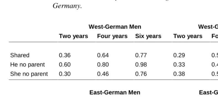
Table 2: Estimated probabilities for having a second child within two, four and six years. Evaluated for calendar year 1980, women aged 23 and men aged 25 in West Germany and women aged 21 and men aged 23 in East Germany.

West-German Men West-German Women Two years Four years Six years Two years Four years Six years

Shared 0.36 0.64 0.77 0.29 0.52 0.63 He no parent 0.60 0.80 0.98 0.33 0.45 0.55 She no parent 0.30 0.46 0.76 0.38 0.50 0.61

East-German Men East-German Women Two years Four years Six years Two years Four years Six years

Shared 0.30 0.60 0.76 0.31 0.58 0.74 He no parent 0.75 0.88 0.92 0.56 0.78 0.84 She no parent 0.50 0.65 0.71 0.77 0.93 0.96

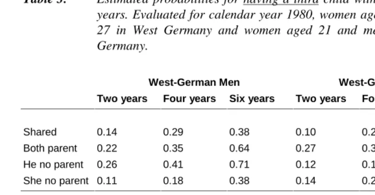
Table 3 gives the estimated probabilities for having a third child for couples with total parity two at the start. Couples with a shared child have the lowest probability of having a third child in all samples apart from West-German men. For West-German women, the probabilities of having a third child in orthodox families and in families where one of the partners is not yet a parent converge for longer durations. In the East-German samples, the childbirth probabilities converge for orthodox families and families where the partner is not yet a parent. Childbirth probabilities in families where the respondent is not yet a parent remain consistently higher than in the two previous groups in East Germany. In all four samples, couples where both partners have already a child from a previous relationship start their childbearing fastest and, apart from West-German men, also continue to have the highest probabilities for having another child. To sum up, the results in Table 3 lend only limited support to the union-confirmation and the parenthood hypotheses especially for longer durations.

(24)

Secondly, the results concerning the parenthood hypothesis are mixed. For short durations couples where one of the partners is not yet a parent have a higher childbirth probability than orthodox families. For longer durations the probabilities of some of these groups do not differ substantially from the childbirth probabilities of orthodox families. Thirdly, the childbirth probabilities of couples where both partners already have a child are higher than expected from the parenthood hypotheses. The very high birth rates of these couples may actually be due to selection into these partnerships; partners who embark on forming such a complex family seem to be willing and desiring to have another child.

Table 3: Estimated probabilities for having a third child within two, four and six

years. Evaluated for calendar year 1980, women aged 25 and men aged 27 in West Germany and women aged 21 and men aged 23 in East Germany.

West-German Men West-German Women Two years Four years Six years Two years Four years Six years

Shared 0.14 0.29 0.38 0.10 0.21 0.27 Both parent 0.22 0.35 0.64 0.27 0.37 0.46 He no parent 0.26 0.41 0.71 0.12 0.17 0.22 She no parent 0.11 0.18 0.38 0.14 0.20 0.26

East-German Men East-German Women Two years Four years Six years Two years Four years Six years

Shared 0.09 0.22 0.33 0.09 0.20 0.29 Both parent 0.53 0.69 0.75 0.58 0.79 0.85 He no parent 0.32 0.44 0.50 0.19 0.32 0.37 She no parent 0.17 0.25 0.29 0.32 0.50 0.56

(25)

show increased childbirth probabilities if the respondent is not yet a parent. In the present paper I can only speculate about reasons for this pattern. A possible explanation takes up the earlier discussed problems of identifying the other parent of respondents’ children. If a child that is classified as a child of the respondent is in fact a shared child of the couple, the birth rate of couples where one partner is no parent yet is underestimated because some of the couples truly follow the lower birth rate of couples with a shared child. However, classifying children born up to three years before the start of the partnership as shared child of the couple reduces the discrepancy between birth rates of couples where the respondent or the partner is not yet a parent, but it does not change the basic pattern (no table).

The proportional hazard models in the present paper are specified exactly as the proportional-hazard model in the paper by Thomson et al. (in press). Differences in the estimates are due to differences in dealing with missing dates because Thomson and co-authors have made no imputations when dates were incomplete. The non-proportional hazard model presented here can be regarded as a test for whether the very high estimated parameters in the German samples in the paper by Thomson et al. are due to a model misspecification. However, the estimated parameters in the non-proportional hazard model are even larger than in the proportional hazard model. In this respect the non-proportional models confirm the conclusions about West Germany in the earlier paper, but they raise questions about the stability of the observed patterns over time at risk.

6. Summary and discussion

(26)

for short-term durations. For longer durations, some of the predicted differences between the types of families do not emerge any more. The different child configurations at the beginning of a partnership seem to indicate different childbearing plans at that time, but the longer the decision to have another child is postponed the less the child configuration seems to matter.

Secondly, the high birth rates of couples formed by two parents demand another modification of the hypotheses formulated at the outset of the paper. The need for a confirmation of the union by a shared child may vary between couples. It may be especially those couples who embark on the adventure of forming a family where both partners bring a child from earlier relationships that the wish and the readiness for a shared child are comparatively high.

The suggested modifications of the union-commitment and the parenthood hypotheses are derived from the model estimated in this paper. Scholars may argue that instead of distinguishing two time patterns in the fertility models it would be better to estimate separate baseline rates for more types of families. The attempt has been made but the number of observations is so small that the estimated parameters are very volatile. Therefore, they are not presented here.

Another possible shortcoming of this paper is that it ignores issues of union stability. Stepfamilies are less stable than families with shared children only. Comparisons of childbirth probabilities between orthodox families and stepfamilies after six years may be misleading because more stepfamilies have dissolved by this time. The short-term differences in birth rates may actually reflect better the true differences in childbearing rates. Further research should incorporate aspects of union stability into models of fertility in stepfamilies and orthodox families.

7. Acknowledgement

(27)

Notes

1. For an overview see Heerkerens (1986).

2. Extending prior childbearing information to both partners causes an additional

problem. As Thomson describes, the NSFH does not provide direct information about the relationship between the current spouse and the respondent’s children who have left home (Thomson 1997). Similar problems occur in the FFS data used in the present study. There is no direct information about the other parent of respondent’s children who have left home.

3. The records are also censored at the conception of a multiple birth.

4. Further details about the data as well as analyses of family formation with the FFS-data are given in Hullen (1995).

5. The calculations are based on counting the number of partners in the partnership histories. Among West-German men, 54% had no partner and 8% had lived with more than two partners. Among West-German women, 39% had never lived with a partner and 8% had more than two partners. The corresponding numbers for East-German men are 31% and 11% and for East-East-German women 24% and 12%.

6. This corresponds to the procedure in Thomson and collaborators (in press).

7. Walter Bien and Markus Teubner (personal communication) have been so kind to

check this interpretation with the data from the German Family Survey (GFS). The GFS provides dates of the beginning of the partnership as well as the dates of moving together. Their computations showed that in nearly all cases when East German men reported a common child born before moving together this child was indeed born after the date of the beginning of the partnership. Therefore, it seems to be appropriate to classify them as shared children of the couple.

(28)

children of the couple, the distributions change in the following way: 7 percent of partnerships of West-German men, and 9, 13, and 15 percent of partnerships of West-German women, East-German men and East-German women have a non-shared child.

10. The estimated slopes dur01, dur12, dur25 and dur5+ have been called s0, s1, s2 and

s3 in section 3.2 and noshad01, noshad12, noshad25, and noshad5+ have been

called sA0, sA1, sA2 and sA3.

11. In the East-German samples there are very few observations for respondents aged 35 and above. Therefore, there is no node at age 35 for East-German respondents.

12. The Figures give approximations of the estimated hazard rates. The values for

complete years are exact. They are connected by smoothed lines unless the smoothing procedure leads to negative values for estimated hazard rates.

(29)

References

Andersen, Per K., Ørnulf Borgan, Richard D. Gill, Niels Keiding. (1992). Statistical Models Based on Counting Processes. New York: Springer.

Bien, Walter, Angela Hartl, Markus Teubner. (2001). Stieffamilien in Deutschland. In: Deutsches Jugendinstitut (ed.). Das Forschungsjahr 2001. München: Deutsches Jugendinstitut e.V.: 87-108.

Blake, Judith. (1979). Is Zero Preferred? American attitudes toward childlessness in the 1970s. Journal of Marriage and the Family, 41: 245-257.

Buber, Isabella and Alexia Prskawetz. (2000). Fertility in Second Unions in Austria: Findings from the Austrian FFS. Demographic Research, http://www.demographic-research.org/Volumes/Vol3/2.

Friedl, Ingrid. (1988). Stieffamilien. München: DJI Verlag Deutsches Jugendinstitut e.V.

Furstenberg Jr, Frank F. (1987). Fortsetzungsehen. Ein neues Lebensmuster und seine Folgen. Soziale Welt, 38: 29-39.

Ganong, Lawrence H. and Marylin Coleman. (1994). Remarried Family Relationships. Thousand Oakes: Sage.

Griffith, Janet D., Helen P. Koo, C. M. Suchindran. (1985). Childbearing and Family in Remarriage. Demography 22: 73-88.

Heekerens, Hans-Peter. (1986). Generatives Verhalten Wiederverheirateter. Zeitschrift

für Bevölkerungswissenschaft 12: 503-517.

Hobcraft, John, Kathleen Kiernan. (1995). Becoming a Parent in Europe. Discussion Paper WSP/116, Welfare State Program, London School of Economics.

Hullen, Gert. (1995). Lebensverläufe in West- und Ostdeutschland. Opladen: Leske+Budrich.

(30)

Lillard, Lee A., Constantijn W. A. Panis. (2000). aML Multilevel Multiprocess Statistical Software, Release 1.0. Los Angeles: EconWare.

Nave-Herz, Rosemarie. (1994). Familie heute. Wandel der Familienstrukturen und Folgen für die Erziehung. Darmstadt: Wissenschaftliche Buchgesellschaft.

Pohl, Katharina. (1995). Familienbildung und Kinderwunsch in Deutschland – Design und Struktur des deutschen FFS, Materialien zur Bevölkerungswissenschaft Heft 82a, Federal Institute for Population Research, Wiesbaden.

Schneider, Norbert F., Walter Bien. (1998): Nichteheliche Elternschaft – Formen, Entwicklung, rechtliche Situation. In: Walter Bien, Norbert Schneider (eds.). Kind ja, Ehe nein?. Opladen: Leske + Budrich: 1-40.

Thomson, Elizabeth. (1997). Her, His and Their Children: Influences on Couple Childbearing Decisions. NSFH Working Paper No. 76, Center for Demography and Ecology, University of Wisconsin-Madison.

Thomson, Elizabeth, Jan M. Hoem, Amy Godecker. (1999). Selection Processes in Stepfamily Fertility. Paper presented at the European Population Conference, The Hague, The Netherlands, August 29-September 4, 1999.

Thomson, Elizabeth, Jan M. Hoem, Andres Vikat, Isabella Buber et al. (in press). Childbearing in Stepfamilies: How Parity Matters. In: E. Klijzing and M. Corijn (eds.). Fertility and partnership in Europe: findings and lessons from comparative research. Volume II. Geneva/New York: United Nations.

Vikat, Andres, Elizabeth Thomson, Jan M. Hoem. (1999). Stepfamily Fertility in Contemporary Sweden: The impact of childbearing before the current union.

Population Studies 53: 211-225

Walper, Sabine. (1993). Stiefkinder. In: Markefka, Manfred, Bernhard Nauck. (eds.). Handbuch der Kindheitsforschung. Neuwied: Luchterhand: 429-438.

Wineberg, Howard. (1990). Childbearing after Remarriage. Journal of Marriage and

(31)

Appendix A: Overview over sample selection. Numbers refer to stepwise exclusion.

West Men West Women East Men East Women

Number of respondents 2024 3012 1992 2984 Number of partnershipsa 1154 2204 1648 2743 respondent’s number of

ships unclearb

26 60 27 30

East-German partnerships that start after January 1990

179 228

start year of partnership missing 13 26 70 138 end date of partnership missing c 27 59 44 78 end date of previous partnership

missing

11 15 9 14

unions overlapd 12 15 10 33

births less 7 months apartd ₄ ₇ ₁₄ ₈

under 14 years at eventde 13 17 22 14 7 months before interviewf ₁₄ ₃₀ ₀ ₀

type of child born before partnership not given

48 88 111 147

child cannot be classifiedg 13 47 33 48 non-shared child born during

partnership

11 14 12 25

spouse’s number of pre-union children missing or different from child history

9 22 11 23

Resulting number of partnerships 952 1804 1106 1958 These consist of three types:

stepfamily 84 203 308 514

childless throughout partnersh. 450 662 252 279 no stepfamily, shared child 418 939 546 1165

Notes: a Number of partnership spells reported in the partnership history.

b Total number of partnerships or total number of marriages missing; also five respondents with missing or implausible histories excluded.

c End date of partnership missing, or equal start date, or precedes start date. d All partnerships of the respondent are excluded.

(32)

Appendix B: Log-linear hazard rate models for childbirth. Proportional and non-proportional models for West-German sample. Standard errors in parentheses.

West-German Men West-German Women

Proportional Non-proportional Proportional Non-proportional

dur01 1.571 *** 1.706 *** 1.170 *** 1.503 ***

(.418) (.453) (.226) (.262)

dur12 .045 .127 .150 .205

(.214) (.222) (.134) (.140)

dur25 -.103 -.137 -.225 *** -.230 ***

(.085) (.086) (.054) (.057)

dur5+ -.255 ** -.245 ** -.386 *** -.458 ***

(.105) (.105) (.068) (.081)

totpar2 -1.111 *** -1.114 *** -1.137 *** -1.146 ***

(.156) (.157) (.098) (.099)

totpar3 -1.737 *** -1.726 *** -1.175 *** -1.194 ***

(.366) (.376) (.190) (.192)

totpar4+ -1.713 * -1.699 * -2.511 *** -2.522 ***

(.908) (.921) (.701) (.709)

noshared .696 1.599 .988 ** 2.604 ***

(.718) (1.308) (.425) (.628)

shenopar -.930 -.777 -.801 * -.737

(.813) (.842) (.456) (.509)

henopar .018 .178 -.936 ** -.894 *

(.767) (.895) (.452) (.502)

shared1+ .140 .144 .647 *** .647 ***

(.427) (.438) (.211) (.211)

shared2+ 1.857 *** 1.868 *** .483 .481

(.522) (.521) (.435) (.444)

wage<25 -.079 ** -.080 ** -.042 * -.049 **

(.038) (.039) (.022) (.022)

wage2530 -.012 -.013 -.012 -.004

(.057) (.058) (.037) (.038)

wage3035 -.223 * -.221 * -.049 -.078

(.119) (.121) (.090) (.094)

wage35+ -.069 -.069 -.589 -.580

(.199) (.198) (.541) (.545)

mage<25 .054 .051 .007 .005

(.052) (.053) (.030) (.030)

mage2530 -.045 -.044 .049 * .050 *

(.054) (.054) (.026) (.026)

mage3035 .144 .145 -.037 -.034

(.103) (.103) (.038) (.040)

mage35+ .439 .504 -.013 -.004

(.364) (.408) (.039) (.041)

bef1980 .131 * .132 * .017 .020

(.076) (.077) (.032) (.032)

aft1980 -.039 ** -.041 ** .019 .020 *

(.019) (.019) (.011) (.012)

constant -3.740 *** -3.847 *** -2.628 *** -2.897 ***

(33)

Appendix B: Log-linear hazard rate models for childbirth. Proportional and non-proportional models for West-German sample. Standard errors in parentheses. (Continued)

West-German Men West-German Women

Proportional Non-proportional Proportional Non-proportional

noshad01 -.709 -1.554 ***

(1.209) (.585)

noshad12 -1.983 -1.162 **

(1.250) (.547)

noshad25 .946 .269

(.618) (.194)

noshad5+ -.359 .397 ***

(1.539) (.150)

ln-L -1588.6 -1583.6 -3806.0 -3784.9

(34)

Appendix C: Log-linear hazard rate models for childbirth. Proportional and non-proportional models for East-German sample. Standard errors in parentheses.

East-German Men East-German Women

Proportional Nonproportional Proportional Nonproportional

dur01 .484 * 1.051 * .994 *** 1.592 *

(.250) (.352) (.178) (.239)

dur12 .268 .365 * .203 * .173

(.186) (.206) (.120) (.130)

dur25 -.015 -.007 -.087 * -.060

(.067) (.069) (.045) (.049)

dur5+ -.324 *** -.355 * -.089 * -.104 *

(.097) (.098) (.047) (.050)

totpar2 -1.292 *** -1.295 * -1.343 *** -1.357 *

(.157) (.159) (.096) (.097)

totpar3 -1.468 *** -1.502 * -1.444 *** -1.430 *

(.243) (.245) (.187) (.191)

totpar4+ -.451 -.490 -1.525 *** -1.564 *

(.302) (.299) (.357) (.366)

noshared 1.703 *** 3.243 * 2.073 *** 3.522 *

(.263) (.448) (.198) (.341)

shenopar -1.343 *** -1.392 * -.744 *** -.821 *

(.338) (.389) (.217) (.241)

henopar -.577 ** -.684 * -1.462 *** -1.396 *

(.282) (.337) (.210) (.231)

shared1+ 1.281 *** 1.275 * 1.072 *** 1.084 *

(.194) (.195) (.137) (.137)

shared2+ .138 .156 -.150 -.165

(.346) (.349) (.319) (.320)

wage<25 -.063 * -.083 * -.034 -.044 *

(.035) (.035) (.022) (.022)

wage2530 -.065 -.042 -.157 *** -.145 *

(.055) (.059) (.041) (.042)

wage3035 .002 .019 -.265 ** -.259 *

(.092) (.104) (.130) (.131)

wage35+ -.178 -.153

(.156) (.156)

mage<25 .064 .050 -.008 -.015

(.043) (.043) (.029) (.029)

mage2530 .040 .051 -.003 -.004

(.042) (.044) (.024) (.024)

mage3035 -.094 -.093 .008 .015

(.103) (.105) (.033) (.033)

mage35+ -.054 ** -.043

(.026) (.029)

bef1980 -.001 .002 .051 * .050 *

(.052) (.052) (.028) (.029)

aft1980 -.068 *** -.067 * -.045 *** -.044 *

(.019) (.019) (.012) (.012)

constant -2.173 *** -2.493 * -2.601 *** -3.003 *

(35)

Appendix C: Log-linear hazard rate models for childbirth. Proportional and non-proportional models for East-German sample. Standard errors in parentheses. (Continued)

East-German Men East-German Women

Proportional Nonproportional Proportional Nonproportional

noshad01 -1.292 * -1.607 *

(.546) (.392)

Noshad12 -.729 .064

(.554) (.334)

Noshad25 -.273 -.343 *

(.306) (.173)

noshad5+ -.212 .054

(1.143) (.129)

ln-L -2850.8 -2832.7 -5037.3 -5016.1

(36)