* Corresponding author: Tel: +982148252195 Email:[email protected]
Application of Box Behnken Design to Optimize the
Parameters to Synthesis Graphene by CVD Process
Ahmad Ghozatloo*1, Zeynab Hajjar1, Mojtaba Shariaty Niassar2 and Ali Morad Rashidi1
1
Research Institute of Petroleum Industry (RIPI), West Blvd. Azadi Sport Complex, Tehran, I. R. Iran
2
Transport phenomena and Nanotechnology Laboratory, Department of Chemical Eng, University of Tehran, Tehran, I. R. Iran
(Received 09 September 2014, Accepted 08 November 2015)
Abstract
This paper discusses the use of Box Behnken design (BBD) approach to plan the experiments for turning the yield of CVD, thickness and layer number of graphene sheets with an overall objective of optimizing the process to provide higher graphene production volume, fewer layers and thinness structure of graphene. BBD is having the maximum efficiency for an experiment involving four factors such as total gas flow, gas ratio (H2/CH4), temperature, and reaction time in three levels. The proposed BBD requires 25 runs of experiment for data acquisition and modeling the response surface. Three regression models were developed and their adequacies were verified to predict the output values at nearly all conditions. Further, the models were validated by performing experiments, taking three sets of random input values. The output parameters measured through experiments (actual) are in good consistency with the predicted values using the models. This work resulted in identifying the optimized set of turning parameters for CVD process to achieve high yield value and good structure of graphene. In the best condition, yield of process is 6.1%.
Keywords
: Box-behnken, CVD, Graphene, Optimization, Yield.1. Introduction
Graphene, one of the allotropes of elemental carbon, is a flat monolayer of sp2-bonded carbon atoms in a two-dimensional (2D) structure. Graphene has exhibited some unusual behaviors, such as very high carrier mobility [1], long-range ballistic transport at room temperature [2], quantum confinement in nanoscale ribbons [3], and single-molecule gas detection sensitivity [4]. These peculiar properties of graphene give it capability to enhance the mechanical and electrical properties of other compounds as an excellent additive. Graphene has demonstrated a variety of intriguing properties including high electron mobility at room temperature (250,000 cm2/Vs) [4] exceptional thermal conductivity (5000W/mK) and superior mechanical properties with Young’s modulus of 1 TPa. Therefore, graphene has various potential applications such as in large-scale assembly and field effect devices [5]. In general, there are three main groups to synthesize graphene, including
exfoliation and cleavage, chemical vapor deposition (CVD) and chemically derived graphene (CDG). Group of exfoliation and cleavage consist of mechanical exfoliation in solutions [6] and intercalation of small molecules by mechanical exfoliation. CVD category consist of Thermal CVD [7], Plasma enhanced CVD [8] and Thermal decomposition on substrates [9].
One of the most important stages in development of an efficient production of grapheme is optimization of reaction parameters for economic production of high value products from renewable sources. Response surface methodology (RSM) is an effective optimization tool wherein many factors and their interactions can be identified with fewer experimental trials [19-20].
The optimization process of this methodology involves studying the response of statistically designed combinations, estimating the coefficients by fitting it in mathematical model that fits best the experimental conditions, predicting the response of the fitted model, and checking the adequacy of the model. Now, Central composite design (CCD) [21] and Box-Behnken design (BBD) [22] are amongst the most commonly used in various experiments.
BBD allows calculation of the response to be made at intermediate levels which were not experimentally studied. No modeling has been done using BBD to synthesis of carbon nanostructures.
In this study four variables in three levels BBD were employed and the optimal conditions were determined through a minimal experiment number compared with other designs [23].
Developing the models for prediction of CVD yield is one of more important objective of this research and so thickness, layer number of graphene sheets. Further, the models were validated with different set of experimental values based on the experimental data. Surface plots were generated to explain the trend of achievable the yield, thickness and layer number of graphene sheets under specific combination of process parameters.
Ultimately this is useful in understanding the influence of process parameters and the resulting output parameters; further enables in determining the optimum set of process parameters such as temperature, time, total gas flow and feed gas ratio.
2. Experimental Studies
2.1. Materials
Copper foil (30-micrometer thickness) was purchased from Aldrich. Acetic acid, hydrochloric acid and H2O2 were from
Merck KGaA (Darmstadt, Germany). Methane and hydrogen gases with purification of 99.99% were from an Iranian gas corporation and deionized water was used in this study as a base fluid.
2.2. Synthesis of graphene by CVD
The Graphene nanosheets were grown on copper foil by catalytic decomposition in a quarts tube furnace system by CVD method. Before the loading into the furnace, the copper foils were pretreated by acetic acid 25% and mixed up by using a magnetic stirrer for several hours. Then, the copper foils were filtered from acid solution and washed with deionized water until the pH level of copper foils would reach a value of 7. Finally, the soaked copper foils were dried in vacuum oven at 90°C for 2 h [24]. Total gas flow, temperature, time and gas ratio are as independent variables of CVD process which will be evaluated in this paper. These variables had three levels as given in Table 1. The levels were fixed based on the preliminary experiment trials and also the available literatures.
Table 1: Independent variables of CVD process with their values
Level Time (min) Temp. (°C) Total Gas Flow (sccm) Gas ratio (H2/CH4)
1 15 950 500 0.5
2 30 1000 1000 1
3 45 1050 1500 2
300°C /min after growth and the methane and hydrogen gas flows were continued throughout the cooling process. Afterwards, copper particles should be removed by purification treatment. Such purification includes the process of using HCl 50% at 40°C with a magnetic stirrer for 16 h. Then, the contents of the flask filtered by vacuum filtration and washed out by distillated water reaching to PH= 7. After that the filter cake was dried in vacuum oven at 40°C for 8h.
2.3. Box Behnken Design of Experiment
For this approach, Design-Expert software was used to design the experiment and randomize the runs. On the basis of the BBD, the CVD process variables (total gas flow, gas ratio, temperature, and time duration) in the turning process could be optimized with a minimum number of experimental runs with an objective of achieving higher the yield, low layer structure and smallest size of graphene. Design expert software (Version 7, Stat-Ease Inc., Minneapolis, USA), was used. Based on table 1 the proposed BBD requires 25 runs for modeling response surface. The experiments were conducted on CVD for the set of input parameters under the 25 conditions given by BBD.
2.4. Evaluation of Graphene structure
Yield of CVD process is defined as the mass percent of graphene in the end product based on used bed of Catalyst (Cu). Yield of the process gravimetrically determined for each runs [18].
This can be predicted by Von Weimarn ratio, where Yield = (m2 – m1)/m1*100.
Where m1 is the weight of catalyst before
loading and m2 is the weight of catalyst and
graphene after CVD process. X-ray diffraction (XRD) analysis of graphene revealed a variety of information on interlayer distances and the number of graphene layers [17]. In this study, the graphene thickness was calculated from XRD pattern. Figure1 shows the XRD pattern of graphene from run 8.
Figure1: XRD pattern of graphene at 30 min &950°C (Run 8)
In the XRD pattern of graphene (Fig. 1), the strong and sharp peak at 2 = 26.2 corresponds to an interlayer distance of 3.4A (d002) [24]. The crystalline size
(thickness) of the (002) facet was estimated using Scherrer’s equation as 24 ± 0.5°A (2
= 26.2°) which corresponds to 7.1 layers. Further, high resolution of TEM (HR-TEM) image was counted by the number of graphene layers. Figure2 shows one of the HR-TEM images of graphene (run 8).
Figure2: HR-TEM image of graphene at 30min&950°C (run 8)
According to Figure2, the layered
structure of graphene can be shown clearly and the graphene nanosheets are made by CVD in the run 8 condition have an average 7 layer which have a good agreement with results of the XRD in Figure1.
3. Discussions
of a two level factorial design and incomplete block design. It is useful for statistical modeling and optimization of a response variable of interest, which is a function of three or more independent variables.
Table2: Box-Behnken design for the experiment and their responses
CODE A B C D Y # ψ
Run Time (min) Temp (°C) Gas Flow (sccm) Gas ratio (H2/CH4)
Y (%) Layer Thickness (nm)
1 30 1000 1000 1 5.89 5.7 1.9 2 30 1050 1000 0.5 5.88 5.7 1.9 3 45 1000 1000 2 5.56 6.4 2.2 4 15 950 1000 1 4.85 7.8 2.7 5 15 1000 1500 1 5.17 6.1 2.1 6 30 1050 1000 2 5.92 6.1 2.1 7 15 1000 1000 2 5.09 6.4 2.2 8 30 950 1000 0.5 4.68 7.2 2.4 9 15 1000 500 1 4.74 6.2 2.1 10 45 1000 1500 1 5.78 6.1 2.1 11 30 1050 1500 1 5.54 5.9 1.7 12 45 950 1000 1 4.65 7.8 2.7 13 30 1000 1500 0.5 5.67 6.4 2.2 14 30 1050 500 1 5.49 5.8 2
15 30 1000 1500 2 5.65 5.7 1.9 16 15 1000 1000 0.5 5.2 6.3 2.1 17 30 1000 500 2 4.85 5.9 2 18 45 1000 1000 0.5 5.66 6.7 2.3 19 30 1000 500 0.5 5.64 6.6 2.2 20 30 950 500 1 4.69 7.2 2.8 21 30 950 1500 1 5.23 7.1 2.4 22 45 1050 1000 1 5.66 6.4 2.2 23 15 1050 1000 1 5.15 6.4 2.2 24 45 1000 500 1 5.33 5.8 2 25 30 950 1000 2 4.62 7.4 2.5
Moreover, Box-Behnken designs allow estimating coefficients in a second degree polynomial regression and modeling of a quadratic response surface.
The response surface can be further used for process optimization, identification of maximum or minimum responses, and significance of each involved factor, or their
combination. Furthermore, response surfaces can be used for calculating responses not only at experimentally investigated points, but also at any point on the surface. In this work a four factor-three level Box-Behnken design, with 1 replicate at the center point, and 25 runs in total (Table 2) has been used.
3.1. Statistical Analysis and predicted model for CVD yield
The summary of fit and analysis of variance (ANOVA) for CVD yield are given in Table 3 and Table 4, respectively. As can be seen from Table 3, the CVD yield model is in good agreement with actual data obtained in experiments. Moreover, Table 3 shows that the model is significant which is justified by small p-value. Table 3 shows Analysis of variance for Response Surface Reduced Quadratic Model of CVD yield with four predictors:
Table3: Analysis of variance for Response Surface Reduced Quadratic Model of CVD yield
Source Sum of Squares df
Mean
Square F Value p-value Model 3.89 7 0.56 9.6 < 0.0001 A-Time 0.5 1 0.5 8.58 0.0094
B-Tem 2.02 1 2.02 34.89 < 0.0001 C-Flow rate 0.78 1 0.78 13.51 0.0019 D-Gas ratio 0.14 1 0.14 2.47 0.1347 CD 0.29 1 0.29 5.06 0.038
A2 0.2 1 0.2 3.48 0.0495 B2 0.35 1 0.35 6.06 0.0248 Residual 0.98 17 0.058 - -
Cor Total 4.87 24 - - -
The Model F-value of 9.60 implies the model is significant. There is only a 0.01% chance that this large amount of "Model F-Value" could occur due to noise. Values of "Prob > F" less than 0.0500 indicate model terms are significant. In this case A, B, C, CD, A2, B2 are significant model terms. Values greater than 0.1000 indicate the model terms are not significant. If there are many insignificant model terms (not counting those required to support hierarchy).
Table 4: Summary statistics for CVD yield Std. Dev. 0.24 R-Squared 0.79813 Mean 5.29 Adj R-Squared 0.71501 C.V. % 4.54 Pred R-Squared 0.42095 PRESS 2.81 Adeq Precision 10.5874
This may indicate a large block effect or a possible problem with the model and/or data. "Adeq Precision" measures the signal to noise ratio. A ratio greater than 4 is desirable. The ratio of 10.587 indicates an adequate signal. This model can be used to navigate the design space. Equation (1) indicated the final equation in terms of actual factors for prdiciting the CVD yeild of graphene:
Yeild=-102.53+0.0637A+0.20651B-
0.0003255C-0.84D+0.0007CD-0.000835A2-0.00009916B2 (1)
According to the model, Time, Temperature, Flow rate, Gas ratio, binary interaction of Flow rate and Gas ratio and also Time and Temperature squared were significant parameters.
Figure.3: One factor effect plot of parameters on CVD yield
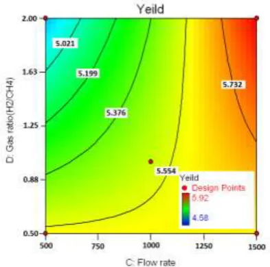
The strength or effect of process parameters is better revealed by one factor effect plot and contour plot of interaction effect of A and C in Figure3., and Figure4 respectively.
3.2. Statistical Analysis and predicted model for graphene layers
The summary of fit and analysis of variance (ANOVA) for graphene layers were given in Table 5 and e 6, respectively. As can be seen from Table 5, the graphene layers model is in good agreement with actual data obtained from the experiments. Moreover, Table 4 shows that the model is significant which is justified by small p-value.
Figure.4: Interaction plot of interaction effect of A and C
Table5: Analysis of variance for Response Surface Reduced Quadratic Model of graphene
layers
Source Sum of Squares df
Mean
Square F Value p-value
Model 8.67 6 1.446084 23.5 < 0.0001
A-Time 0 1 0 0 1.0000
B-Temp 5.60 1 5.603333 91.2 < 0.0001 Gas ratio 0.08 1 0.083333 1.3 0.2592
A2 1.02 1 1.022521 16.6 0.0007 B2 2.79 1 2.796807 45.5 < 0.0001 D2 0.38 1 0.381796 6.2 0.0226 Residual 1.10 18 0.061394 - -
Cor Total 9.78 24 - - -
noise. The fact that values of "Prob > F" is less than 0.0500 indicate model terms are significant and Values greater than 0.1000 indicate the model terms are not significant. In this case B, A2, B2, D2 are significant model terms.
Table6: Summary statistics for graphene layers Std. Dev. 0.247 R-Squared 0.887 Mean 6.444 Adj R-Squared 0.849 C.V. % 3.845 Pred R-Squared 0.782 PRESS 2.127 Adeq Precision 14.498
Table 6 showed Summary statistics for graphene layers. The "Pred R-Squared" of 0.7825 is in reasonable agreement with the "Adj R-Squared" of 0.8494. "Adeq Precision" measures the signal to noise ratio. A ratio greater than 4 is desirable. The ratio of 14.499 indicates an adequate signal. This model can be used to navigate the design space. Equation (2) indicated the final equation in terms of actual factors for prdiciting the nambers of graphene layers:
Layer=325.77-0.12235A-0.62073B-0.000033C-1.544D+0.00204A2+0.00030353B2+0.573D2 (2)
Figure.5: One factor effect plot of parameters on Graphene layers
According to the model significant parameters are Time, Temperature, Flow rate, and also Time, Temperature and Flow rate squared. The effect of process parameters is better revealed by one factor effect plot illustrated in Figure5.
4. Optimization
Simplex optimization and response surface methodology are two main different strategies for optimization. An exact optimum can only be determined by response surface methodology, while the simple method will encircle the optimum. Response surfaces are used to determine an optimum. In addition, it would be good idea to graphically illustrate the relation between different experimental variables and responses. Optimization of one response can be performed numerically for simultaneous optimization of multiple responses. Numerical Optimization will optimize any combination of one or more goals which in this work was performed on basis of DOE software to figure out the optimal conditions of Time, Temperature, Flow rate, Gas ratio on the yield and the numbers of graphene layers. The constraints of this problem were the same as design table, which were selected as the lower and upper bounds of the independent variables.
Table7: Summary for constrains for Yield and Graphene layers optimizations
Name Goal Lower
Limit Upper
Limit Lower Weight
Upper Weight Impo
Time range 15 45 1 1 3
Tempe range 950 1050 1 1 3 Flow rate range 500 1500 1 1 3 (H2/CH4) range 0.5 2 1 1 3
Yield max 4.58 100 1 1 3 G layers min 5.7 7.8 1 1 3 Thickness mini 1.7 2.8 1 1 3
After optimization, the results were gathered in Table 7, which showed the optimal point for Time, Temperature, Flow rate and Gas ratio that means that the maximum yield and minimum graphene layers is occurred in the mentioned operating conditions.
Figure6: Optimized condition to have maximum yield and minimum graphene layers
5. Conclusion
To produce of graphene by CVD process, the optimized condition is 30 min of reaction time, 1030C of reactor temperature, Gas ratio (H2/CH4) of 1.9 and
flow rate of 1500 sccm. In this condition the yield of process is 6.1% and Graphene can produce with 5.7 layers structure.
The graphene layers are strong function of reaction time and temperature. With increasing of 10 min in reaction time, 0.4 layers added to graphene layers. Also with increasing of 100C in reaction temperature, 1.5 layers added to graphene structure. The
graphene layers are weak and reverse function of gas flow rate. By increasing of flow rate, first the graphene layers decreases and then increase. The Optimal value of flow rate is 1.3. Lower layers of graphene can achieve by reducing the reaction time and temperature. The ratio of carrier gas (H2) must be maximum 30% greater than of
the carbon feed and tried to send the additional amount of flow needed into the reactor. So there is not observed any shortcomings in the system for the flow overhead of copper foils.
The yield of process is strong function of reaction time and temperature. The yield of process, first increase and then decreases by increasing of reaction time or temperature. The Optimal condition for flow time is 45 min and for temperature is 1050C. Also the yield of process is weak function of flow rate and reverse function of carrier gas amount. To achieve maximum yield of reaction time should be set up to 45 min and temperature around 1050° C. Also yield increase slightly by increasing of the carbon content of feed. Reaction time and temperature must be reduced as much as possible to achieve a narrow and low layers structure of graphene. Therefore the maximum time is 45 min and temperature is 1050°C is recommended. Further increase amount of carbon in the feed has no significant effect on graphene structure and the yield of process. The carrier gas should be 30% more than carbon feed. It is the best rate of mixing which is recommended. During the reaction time flow should be established as sufficient amount base on the size of internal volume of reactor. In this condition, the graphene structure with maximum efficiency is obtained.
References
1. K.S. Novoselov, A.K. Geim, S.V. Morozov, D. Jiang, Y. Zhang, S.V. Dubonos, I.V. Grigorieva, A.A. Firsov, (2004). “Electric field effect in atomically thin carbon films.” J. Science., Vol. 6, No. 13, pp. 666-672. 2. C. Berger, Z. Song, X.Li, X. Wu, N. Brown, C. Naud, D. Mayou, T. Li, J. Hass, A.N. Marchenkov, E.H.
3. Z Chen, YM Lin, MJ Rooks, P Avouris Physica E, (2007). “Low-dimensional Systems and Nanostructures.”
J. Carbon., Vol. 40, No. 1, pp. 911-928.
4. F. Schedin, A.K. Geim, S.V. Morozov, E.W. Hill, P. Blake, M.I. Katsnelson, L.S. Novoselov, (2007). “Detection of individual gas molecules adsorbed on graphene.” J. NatureMater., Vol. 6, No. 1, pp. 652. 5. Li X, Wang X, Zhang L, Lee S, Dai H. (2008). “Chemically derived, ultrasmooth graphene nanoribbon
semiconductors.” J. Science., Vol. 319, No. 1, pp. 1229.
6. Fukushima H, Drzal LT. (2003). “A carbon nanotube alternative, graphite nanoplatelets as reinforcements for polymers.” J. AnnuTechConf Soc Plast Eng., Vol. 61, No. 36, pp. 2230-2241.
7. Stankovich S, Dikin DA, Piner RD, Kohlhaas KA, Kleinhammes A, Jia Y., (2007). “Synthesis of graphene-based nanosheets via chemical reduction of exfoliated graphite oxide.” J. Carbon , Vol.45, No. 1, pp. 1558-1566.
8. Wang JJ, Zhu MY, Outlaw RA, Zhao X, Manos DM, Holoway BC., (2004). “Synthesis of carbon nanosheets by inductively coupledradio-frequency plasma enhanced chemical vapor deposition.” J. Carbon., Vol. 42, No. 1, pp. 2867.
9. Forbeaux I, Themlin JM, Debever JM. (1998). “Heteroepitaxial graphite on 6H–SiC (0001), interfaces formation through conductionband electronic structure.” J. Phys Rev B., Vol. 58, No. 1, pp. 16396-402. 10.Stankovich S, Dikin DA, Dommett GHB, Kohlhaas KM, Zimney EJ, Stach EA, (2006). “Graphene-based
composite materials.” J. Nature., Vol. 442, No. 2, pp. 44-52.
11.Stankovich S, Piner RD, Nguyen ST, Ruoff RS., (2006). “Synthesis and exfoliation of isocyanate-treated graphene oxide nanoplatelets.” J. Carbon., Vol. 44, No. 1, pp. 3342-3355.
12.Chen J-H, Cullen WG, Jang C, Fuhrer MS, Williams ED., (2009). “Defect scattering in graphene.” J. Phys Rev Lett., Vol. 102, No. 1, pp. 805-812.
13.Wu J, Pisula W, Mullen K. (2007). “Graphenes as potential material for electronics.” J. Chem Rev., Vol. 107, No. 8, pp. 83-96.
14.Barone V, Hod O, Scuseria GE., (2006). “Electronic structure and stability of semiconducting graphene nanoribbons.” J. NanoLett., Vol. 6, No. 2, pp. 44-59.
15.Cao H, Yu Q, Colby R, Pandey D, Park CS, Lian J, (2010). “Large scale graphitic thin films synthesized on Ni and transferred to insulators: Structural and electronic properties.” J. Appl Phys., Vol. 107, No. 4, pp. 44310-19.
16.Bhaviripudi S, Jia X, Dresselhaus MS, Kong J., (2010). “Role of kinetic factors in chemical vapor deposition synthesis of uniform large area graphene using copper catalyst.” J. NanoLett , Vol. 10, No. 2, pp. 4128-4134. 17.Kim KS, Zhao Y, Jang H, Lee SY, Kim JM, Kim KS, (2009). “Large-scale pattern growth of graphene films
for stretchable transparent electrodes.” J. Nature., Vol. 457, No. 3, pp. 706-717.
18.Li X, Cai W, An J, Kim S, Nah J, Yang D, (2009). “Large-area synthesis of high-quality and uniform graphene films on copper foils.” J. Science., Vol. 324, No. 2, pp. 1312-1319.
20.Long Wu, Kit-lun Yick, Sun-pui Ng, Joanne Yip, (2012). “Application of the Box–Behnken design to the optimization of process parameters in foam cup molding.” J. Expert Systems with Applications., Vol. 39, No. 9, pp. 7585-7596.
21.Ross PJ, (1996). “Taguchi techniques for quality engineering.” McGraw- Hill., New York,
22.Montgomery D.C, (1991). “Design and Analysis of Experiments.” John Wiley and sons., New York,
23.C.H., Dong, X.Q., Xie, X.L., Wang, Y. Zhan, and Y.J., Yao, (2009). “Application of Box-Behnken design in optimisation for polysaccharides extraction from cultured mycelium of Cordyceps sinensis.” J. Food and Bioproducts Processing., Vol. 87, No. 2, pp. 139-151.