Accelerated normal and skew-Hermitian splitting methods for positive definite linear systems

F. Toutounian and D. Hezari

Abstract

For solving large sparse non-Hermitian positive definite linear equations, Bai et al. proposed the Hermitian and skew-Hermitian splitting methods (HSS). They re-cently generalized this technique to the normal and skew-Hermitian splitting meth-ods (NSS). In this paper, we present an accelerated normal and skew-Hermitian splitting methods (ANSS) which involve two parameters for the NSS iteration. We theoretically study the convergence properties of the ANSS method. Moreover, the contraction factor of the ANSS iteration is derived. Numerical examples illustrating the effectiveness of ANSS iteration are presented.

Keywords: Non-Hermitian matrix; Normal matrix; Hermitian matrix; Skew-Hermitian matrix; Splitting iteration method.

1 Introduction

Many problems in scientific computation give rise to solving the linear system

Ax=b, (1)

withA∈Cn×na large non-Hermitian positive definite matrix andx, b∈Cn. We observe that the coefficient matrixAnaturally possesses the Hermitian/skew-Hermitian (HS) splitting

A=H+S,

where

H =1 2(A+A

∗_{) and S =} 1

2(A−A

∗_),

withA∗ being the conjugate transpose ofA. Bai et al. [2] presented the HSS iteration method: Given an initial guess x(0) ∈Cn, fork = 0,1,2, . . ., until

F. Toutounian

Department of Applied Mathematics, Faculty of Mathematical Sciences, Ferdowsi Univer-sity of Mashhad, Mashhad, Iran. e-mail: [email protected]

Davood Hezari

Department of Applied Mathematics, Faculty of Mathematical Sciences, Ferdowsi Univer-sity of Mashhad, Mashhad, Iran. e-mail: hezari [email protected]

31

Accelerated normal and

{x(k)_{}converges, compute}

(αI+H)x(k+12)= (αI−S)x(k)+b,

(αI+S)x(k+1)= (αI−H)x(k+12)+b, (2)

where α is a given positive constant. They have also proved that for any positiveα, the HSS method converges unconditionally to the unique solution of the system of linear equations.

Moreover, based on the HS splitting, Li et al. [5] presented the asymmet-ric Hermitian/skew-Hermitian splitting (AHSS) iteration method: Given an initial guess x(0)∈Cn, fork= 0,1,2, . . ., until {x(k)} converges, compute

(αI+H)x(k+12)= (αI−S)x(k)+b,

(βI+S)x(k+1)= (βI−H)x(k+12)+b, (3)

where αis a given nonnegative constant andβ is a given positive constant. They proved that if the coefficient matrix A is positive definite (Hermitian or non-Hermitian) the AHSS iteration converges to the unique solution of linear system (1) with any given nonnegativeα, ifβ is restricted to an appropriate region.

Bai et al. [1] recently generalized the HS splitting to the normal/skew-Hermitian (NS) splitting

A=N+S, (4)

where N ∈ Cn×n is a normal matrix and S ∈ Cn×n is a skew-Hermitian matrix, and obtained the following normal/skew-Hermitian splitting (NSS) method to iteratively compute a reliable and accurate approximate solution for the system of linear equations (1):

The NSS iteration method:Given an initial guessx(0)∈Cn. Fork= 0,1,2. . . until{x(k)} converges, compute

(αI+N)x(k+12)= (αI−S)x(k)₊b,

(αI+S)x(k+1)= (αI−N)x(k+12)+b, (5)

where α is a given positive constant. They have also proved that for any positiveαthe NSS method converges unconditionally to the unique solution of the system of linear equations.

skew-Hermitian, but it is not dependent on the eigenvectors of the matricesN, S andA.

The organization of this paper is as follows. In section 2, we establish the ANSS iteration and study its convergence properties. Numerical experiments are presented in section 3 to show the effectiveness of our method. Finally, in section 4, some concluding remarks are given.

2 The ANSS Method

Throughout the paper, the non-Hermitian matrix A∈Cn×n ( i.e. A=A∗) is positive definite if its Hermitian part is Hermitian positive definite.

Based on the NSS iteration (5), in this paper we present a new approach to solve the system of linear equations (1), called the ANSS iteration, and it is as follows.

The ANSS iteration method: Given an initial guess x(0) ∈ Cn, for k = 0,1,2. . . until{x(k)}converges, compute

(αI+N)x(k+12)= (αI−S)x(k)+b,

(βI+S)x(k+1)= (βI−N)x(k+12)+b, (6)

whereαis a given nonnegative constant andβ is a given positive constant. The ANSS iteration alternates between the normal matrix N and the skew-Hermitian matrixS. In fact, we can reverse the roles of the matricesN andS in the above ANSS iteration so that we may first solve the system of linear equations with coefficient matrixβI+S and then solve the system of linear equations with coefficient matrixαI+N.

Note that both αI+N and βI+S are normal matrices. Therefore, the linear systems with the coefficient matrices αI +N and βI +S may be solved accurately and efficiently by some Krylov subspace iteration methods, e.g. GMRES. It is known that the GMRES method naturally reduces to an iterative process of the three-term recurrence. See [4, 3] for other iteration methods about solving large sparse normal system of linear equations.

In matrix-vector form, the ANSS iteration method can be equivalently rewritten as

x(k+1)_{=M(α, β)x}(k)_{+G(α, β)b, k= 0,1,2, . . . , (7)}

where

M(α, β) = (βI+S)−1(βI−N)(αI+N)−1(αI−S) (8)

and

Here, M(α, β) is the iteration matrix of the ANSS iteration. In fact, (7) may also result from the splitting

A=B(α, β)−C(α, β)

of the coefficient matrixA, with ⎧

⎪ ⎪ ⎪ ⎨ ⎪ ⎪ ⎪ ⎩

B(α, β) = 1

α+β(αI+N)(βI+S)

C(α, β) = 1

α+β(βI−N)(αI−S).

(9)

Obviously

M(α, β) =B(α, β)−1_{C(α, β) and G(α, β) =B(α, β)}−1_.

To study the convergence properties of the ANSS iteration and derive the upper bound of the contraction factor, we first represent the following lem-mas.

Lemma 2.1.Let α be a nonnegative constant and β be a positive constant. If (γ, η)∈Ω, whereΩ= [γ_min, γ_max]×[η_min, η_max], γ_min >0 and η_min≥0, then

f(α, β)≡ max

(γ,η)∈Ω _(β

−γ)2_+η2

(α+γ)2+η2

= ⎧ ⎪ ⎪ ⎪ ⎪ ⎨ ⎪ ⎪ ⎪ ⎪ ⎩

max

γmin≤γ≤β−2α

_(β

−γ)2_+η2 min

(α+γ)2+η_min2

for γ_min≤ β−α 2

max

γmin≤γ≤γmax

_(β

−γ)2_+η2 max

(α+γ)2+η_max2

for β−α

2 ≤γmin.

(10)

Proof. Let us define the functiong(η) by

g(η) = (β−γ)2+η2 (α+γ)2+η2.

Differentiation gives

g_{(η) =} 2η(α+β)(α−β+ 2γ)

[(α+γ)2+η2]2 .

Since (α+β)>0, it follows that the functiong(η) is an increasing function

ifγ≥β−α

2 and is a decreasing function ifγ≤ β−α

If β−α

2 ≤ γmin, then for all γ satisfying γmin ≤ γ ≤ γmax, we have β−α

2 ≤ γ. So, for γmin ≤ γ ≤ γmax, the function g(η) is an increasing function, and

f(α, β) = max

γmin≤γ≤γmax

_(β

−γ)2_+η2 max

(α+γ)2+η_max2

if γ_min≤ β−α

2 . (11)

If γ_min ≤ β−α

2 , then, by using β +α > 0, for all γ satisfying γmin ≤ β−α

2 ≤γ,we obtain (β−γ)

2_≤(α+γ)2_{, which implies that}

(β−γ)2_+η2

(α+γ)2+η2 ≤1.

Similarly, for allγsatisfyingγ_min≤γ≤ β−α

2 , we obtain (β−γ)

2_≥(α+γ)2

and

(β−γ)2_+η2

(α+γ)2+η2 ≥1. Therefore,

f(α, β) = max

γmin≤γ≤β−2α,ηmin≤η≤ηmax

_(β−γ)2 +η2 (α+γ)2+η2

, if γ_min≤ β−α 2

From the fact that, for γ_min ≤γ≤ β−α

2 , the function g(η) is a decreasing function, we can conclude that

f(α, β) = max

γmin≤γ≤β−2α

_(β

−γ)2_+η2 min

(α+γ)2+η_min2

, if γ_min≤ β−α

2 (12)

Therefore (11) and (12) immediately result relation (10).

Lemma 2.2.Let α be a nonnegative constant and β be a positive constant. If β−α

2 ≤γmin, where0< γmin, then

max

γmin≤γ≤γmax

(β−γ)2+η2_max (α+γ)2+η2_max

= max

(β−γ_min)2+η2_max (α+γ_min)2+η2_max,

(β−γmax)2+η_max2 (α+γmax)2+η_max2

(13)

Proof. Let us define the functiong(γ) by

g(γ) =(β−γ)2+ηmax2

(α+γ)2+η2_max.

g_{(γ) =}−2(α+β)

−γ2_{+ (β−α)γ+βα+η}2 max

[(α+γ)2+η_max2 ]2 .

The smallest root ofg(γ) is negative and is not in the interval [γ_min, γ_max]. The largest root ofg(γ) is

γ₁= (β−α) +

(β−α)2_{+ 4(βα+η}2 max)

2 .

By simple computation, we can show that this root is a minimum point for the functiong(γ). Hence (13) holds and the proof of Lemma is completed.

Lemma 2.3.Let α be a nonnegative constant and β be a positive constant. If 0< γ_min≤β−α

2 , then

f(α, β) = max

γmin≤γ≤β−2α

_(β

−γ)2_+η2 min

(α+γ)2+η2_min

= (β−γmin)2+η2min (α+γ_min)2+η_min2 .

Proof. Let us define the functionh(γ) by

h(γ) = (β−γ)2+η2min

(α+γ)2+η_min2 .

Differentiation gives

h_{(γ) =} −2(α+β)

(β−γ)(α+γ) +η_min2 [(α+γ)2+η2_min]2

Since (α+β) > 0 and γ ≤ β, for all γ satisfying γ_min ≤ γ ≤ γ_max and γ≤β−α

2 , we haveh

_{(γ)<0. Thus}

f(α, β) =(β−γmin)2+ηmin2 (α+γ_min)2+η2_min.

The following theorem describes the convergence property of the ANSS iteration.

δ(α, β)≡ max

σj∈σ(S)

α2_+σ2

j

β2_+σ2

j

max

γj+iηj∈λ(N)

(β−γ_j)2+η_j2

(α+γ_j)2+η2_j (14)

where λ(N) is the spectral set of N and σ(S) is the singular-value set of

S. Let γ_min and γ_max, η_min and η_max be the lower and the upper bound of the real, the absolute values of the imaginary parts of the eigenvalues of the matrix N, respectively, and σ_min,σ_max be the lower and the upper bound of the singular-value set of the matrix S, respectively. Then δ(α, β)<1 if one of the following conditions holds:

(a) Any given parameterαandβ satisfies

max

_α(γ2

min+ηmax2 )

2αγ_min+γ_min2 +η_max2 ,

α(γ2

max+ηmax2 )

2αγ_max+γ_max2 +η2_max

< β≤α+ 2γ_min

(b) Any given parameterαandβ satisfies

α+ 2γ_min< β

if σ_max≤√γ_min+η_min+ 2γ_minα. (c) Any given parameterαandβ satisfies

α+ 2γ_min< β≤ α(γmin2 +ηmin2 −σ2max)−2σmax2 γmin

γ2

min+ηmin2 −σ2max+ 2αγmin

if σ_max≥√γ_min+η_min+ 2γ_minα.

Proof. By the similarity invariance of the matrix spectrum, we have

ρ(M(α, β)) =ρ((βI−N)(αI+N)−1(αI−S)(βI+S)−1)

≤ (βI−N)(αI+N)−1₂(αI−S)(βI+S)−1₂.

LettingQ(α, β) = (αI−S)(βI+S)−1 and noting thatS∗=−S, we have Q(α, β)∗_{Q(α, β) =(αI−S)(βI+S)}−1 ∗_{(αI−S)(βI+S)}−1

= (βI−S)−1_{(αI+S)(αI−S)(βI+S)}−1

= (αI−S)(βI+S)−1(βI−S)−1(αI+S) =Q(α, β)Q(α, β)∗

That is to say,Q(α, β) is a normal matrix. Therefore, there exists a unitary matrixU ∈Cn×nand a complex diagonal matrix_q = diag(˜λ₁,λ˜₂, . . . ,˜λ_n)∈ Cn×n _{such that Q(α, β) = U}∗

Q(α, β)x= ˜λx (αI−S)(βI+S)−1x= ˜λx (βI+S)−1(αI−S)x= ˜λx

(αI−S)x= ˜λ(βI+S)x

If ˜λ=−1, then

Sx= α− ˜ λβ

1 + ˜λ x (15)

If ˜λ=−1, then

(α+β)x= 0.

Since α+β > 0, it implies x = 0, and this contradicts the definition of eigenvector. Therefore ˜λ=−1 can not be an eigenvalue ofQ(α, β).

From (15), α−λβ˜

1 + ˜λ is an eigenvalue ofSandxis an associated eigenvector. Since S is a skew-Hermitian matrix, its eigenvalues are pure imaginary and thus of the formiτ_j,j= 1, . . . , n, whereτ_j∈R, So

˜

λ_j =α−iτj β+iτ_j,

whereiτ_j is an eigenvalue of S. Therefore

Q(α, β)2=U∗∧qU2= ∧q2= max

σj∈σ(S)

α2_+σ2

j

β2_+σ2

j

. (16)

Because N is a normal matrix, there exists a unitary matrix V ∈Cn×n and a complex diagonal matrix _N = diag(λ₁, λ₂, . . . , λ_n) ∈ Cn×n such that N =V∗_NV.Hence, we have

(αI+N)−1(βI−N)₂= max

λj∈λ(N)

|β−λ_j | |α+λ_j |

= max

λj=γj+iηj∈λ(N)

(β−γ_j)2+η2_j

(α+γ_j)2+η2_j (17)

Now, from (16) and (17), we see that

ρ(M(α, β))≤ max

σj∈σ(S)

α2_+σ2

j

β2_+σ2

j

max

λj=γj+iηj∈λ(N)

(β−γ_j)2+η_j2 (α+γ_j)2+η_j2.

To prove (a), we note that, if β−α

2 ≤γmin, then β−α≤2γ forγmin≤ γ ≤γ_max. By using 0 <(β+α), we obtain (β−γ)2 ≤(α+γ)2. Thus, by Lemma 2.1, we have

f(α, β) = max

γmin≤γ≤γmax

_(β−γ)2 +η_max2 (α+γ)2+η_max2

≤1, for β−α

2 ≤γmin (18)

Moreover, ifβ > α, then max

σj∈σ(S)

α2_+σ2

j

β2_+σ2

j

<1, and therefore

(i) if α < β≤α+ 2γ_min then δ(α, β)<1.

Ifβ ≤α, then max

σj∈σ(S)

α2_+σ2

j

β2_+σ2

j

≤α_β. By using (18), we have

δ(α, β)≤ α_β max

γmin≤γ≤γmax

(β−γ)2_+η2 max

(α+γ)2+η2_max.

So, in order to have the bound δ(α, β) < 1, the following inequality must hold

max

γmin≤γ≤γmax

_(β−γ)2 +η_max2 (α+γ)2+η2_max

< β2

α2. (19)

By using the results of Lemma 2.2, the following inequalities must hold

(β−γ_min)2+η_max2 (α+γ_min)2+η2_max <

β2

α2 and

(β−γ_max)2+η2_max (α+γ_max)2+η2_max <

β2

α2 (20)

By simple computation, we can show that, forα+β >0, these two inequalities hold ifβ satisfies the following inequalities.

α(γ2

min+ηmax2 )

2αγ_min+γ_min2 +η_max2 < β and

α(γ2

max+ηmax2 )

2αγ_max+γ_max2 +η_max2 < β.

Therefore

(ii) if max

_α(γ2

min+η2max)

2αγ_min+γ_min2 +η2_max,

α(γ2

max+η2max)

2αγ_max+γ_max2 +η2_max

< β ≤ α

thenδ(α, β)<1.

Combining (i) and (ii), we have

(iii) if max

_α(γ2

min+ηmax2 )

2αγ_min+γ_min2 +η_max2 ,

α(γ2

max+ηmax2 )

2αγ_max+γ_max2 +η_max2

To prove parts (b) and (c), we note that, ifγ_min≤ β−α

2 , by Lemmas 2.1 and 2.3, we have

f(α, β) = max

γmin≤γ≤β−2α

_(β

−γ)2_+η2 min

(α+γ)2+η2_min

=(β−γmin)2+ηmin2 (α+γ_min)2+η_min2 ≥1,

since (α+γ_min)≤(β−γ_min). On the other hand,

max

σj∈σ(S)

α2_+σ2

j

β2_+σ2

j =

α2_+σ2

max

β2_+σ2

max

<1,

sinceα < β. So, the relation

δ(α, β) =

α2_+σ2 max

β2_+σ2

max

(β−γ_min)2+η_max2 (α+γ_min)2+η_max2 <1

will hold ifαandβ satisfy the following inequality,

(β−γ_min)2+η2_max (α+γ_min)2+η2_max <

β2_+σ2 max

α2_+σ2 max

. (21)

Forα+β >0, this inequality is equivalent to

0<(β−α)(γ_min2 +η2_min−σ_max2 + 2αγ_min) + 2γ_min(α2+σ_max2 ). (22)

Since (β−α)>0, (22) holds ifσ_max≤γ_min2 +η_min2 + 2αγ_min. Thus

(iv) ifσ_max≤γ_min2 +η2_min+ 2αγ_min andα+ 2γ_min≤β, then δ(α, β)<1.

Ifσ_max>γ_min2 +η_min2 + 2αγ_min, then (22) holds ifβ satisfies the following inequality

β < α(γmin2 +η2min−σ2max+ 2αγmin)−2γmin(α2+σmax2 )

γ2

min+ηmin2 −σ2max+ 2αγmin .

Thus

(v) ifσ_max>γ_min2 +η_min2 + 2αγ_min and

α+ 2γ_min≤β≤ α(γmin2 +ηmin2 −σ2max+ 2αγmin)−2γmin(α2+σ2max)

γ2

min+ηmin2 −σ2max+ 2αγmin

then δ(α, β)≤1.

Theorem 2.1 mainly discusses the available β for a convergent ANSS it-eration for any given nonnegative α. It also shows that the choice of β is dependent on the choice of α, the spectrum of the matrix N, the singular-values ofS, but is not dependent on the spectrum ofA. Notice that

α+ 2γ_min− α(γmin2 +ηmax2 )

2αγ_min+γ_min2 +η_max2

= 2αγ

2

min+ 2γ3min+ 2γminη2max+ 2α2γmin

2αγ_min+γ_min2 +η_max2 >0

and

α+ 2γ_min− α(γ2max+ηmax2 )

2αγ_max+γ_max2 +η_max2

=2αγminγmax+ 2γminγmax2 + 2γminη2max+ 2α2γmax 2αγ_max+γ_max2 +η_max2 >0,

we remark that for any given nonnegative α the available β always exists. The bound δ(α, β) of the convergence rate depends on the spectrum of N and S and the choice of αand β. Moreover, δ(α, β) is also an upper bound of the contraction factor of the ANSS iteration.

3 Numerical Example

In this section, we give a numerical example to illustrate the effectiveness of ANSS iteration.

We consider the differential equation

−u+qu=f,

on the inteval [0,1], with the constant coefficient q and the homogeneous boundary condition. When the finite difference discretization, for example, the centered difference is applied to the above equation, we get the system of linear equations (1) with the coefficient matrix

A= tridiag(−1−qh

2 ,2,−1 + qh

2 )

where the equidistant step-sizeh= 1

n+ 1 is used.

LetH =1₂(A+A∗) andS₀= 1₂(A−A∗) be Hermitian and skew-Hermitian parts of A, respectively. We consider a NS splitting

where

N =H+icI and S=S₀−icI

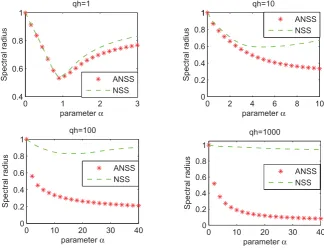
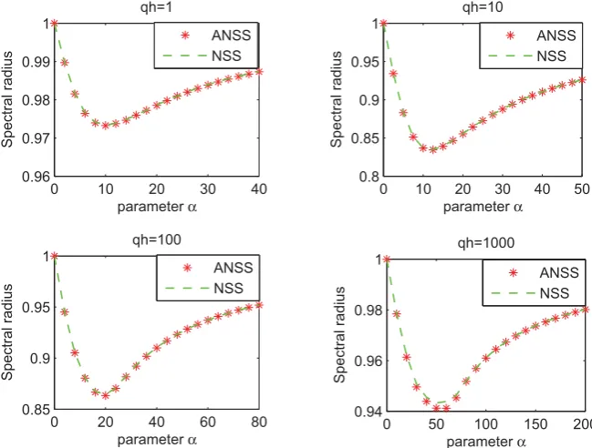
and c is a real number. We test the spectral radius of the iteration matrix M(α, β) (8) with different values ofqh. All the tested matrices are 64×64.

In Figs. 1 and 2, we show the spectral radius of the iteration matrix of the ANSS method and the NSS method with different values of α. ANSS represents the spectral radius of the iteration matrix of the ANSS method, where parameterβ is tested to be the optimal one, and NSS represents that of the NSS method.

0 1 2 3

0.4 0.6 0.8 1

parameterα

Spectral radius

qh=1

0 2 4 6 8 10

0 0.2 0.4 0.6 0.8 1 1

parameterα

Spectral radius

qh=10

0 10 20 30 40

0 0.2 0.4 0.6 0.8 1

parameterα

Spectral radius

qh=100

0 10 20 30 40

0 0.2 0.4 0.6 0.8 1

parameterα

Spectral radius

qh=1000

ANSS NSS ANSS

NSS

ANSS NSS

ANSS NSS

Fig. 1: Spectral radius of iteration matrices of ANSS and NSS methods for c=.1

0 10 20 30 40 0.96

0.97 0.98 0.99 1

parameterα

Spectral radius

qh=1

ANSS NSS

0 10 20 30 40 50

0.8 0.85 0.9 0.95 1

parameterα

Spectral radius

qh=10

ANSS NSS

0 20 40 60 80

0.85 0.9 0.95 1

parameterα

Spectral radius

qh=100

ANSS NSS

0 50 100 150 200

0.94 0.96 0.98 1

parameterα

Spectral radius

qh=1000

ANSS NSS

Fig. 2: Spectral radius of iteration matrices of ANSS and NSS methods for c= 10

4 Conclusion

In this paper, we have introduced two constants for the NSS iteration and presented a different approach to solve the system of linear equations (1), called ANSS method.

Acknowledgment

The authors wish to thank the referee for valuable comments and suggestions.

References

1. Bai, Z-Z. and Golub, G.H. and Ng, M.K.,On successive-overrelaxation acceleration of the Hermitian and skew-Hermitian splitting iterations, Numer. Linear. Algebra. Appl.,₁₄(2007) 319-335.

2. Bai, Z-Z., Golub, G.H. and Ng, M.K.,Hermitian and skew-Hermitian splitting methods for non-Hermitian positive definite linear systems, SIAM J. Matrix. Anal. Appl.,₂₄ (2003) 603-626.

3. Huhtanen, M.,Aspects of nonnormality for iterative methods, Linear Algebra Appl.,

394(2005) 119-144.

4. Huhtanen, M.,A Hermitain Lanczos method for normal matrices., SIAM J. Matrix. Anal. Appl.,23(2002) 1092-1108.