Elimination of Hard-Nonlinearities Destructive Effects in Control Systems Using Approximate Techniques

AUT J. Model. Simul., 50(2) (2018) 117-122 DOI: 10.22060/miscj.2017.12217.5016

Elimination of Hard-Nonlinearities Destructive Effects in Control Systems Using

Approximate Techniques

M. Nazari-Monfared1_{, M. J. Yazdanpanah}2*

1 _{Department of Electrical Engineering, Qazvin Branch, Islamic Azad University, Qazvin, Iran}

2 _{Control & Intelligent Processing Center of Excellence, School of Electrical and Computer Engineering, University of Tehran, Tehran, Iran}

ABSTRACT: Many of the physical phenomena, such as friction, backlash, drag, etc., which appear in mechanical systems are inherently nonlinear and have destructive effects on the control system behavior. Generally, they are modeled by hard nonlinearities. In this paper, two different methods are proposed to cope with the effects of hard nonlinearities which exist in various models of friction. Simple inverted pendulum on a cart (SIPC) is considered as a test bed system, as well. In the first technique, a nonlinear optimal controller based on the approximate solution of Hamilton-Jacobi-Bellman (HJB) partial differential equation (PDE) is designed for the system and finally, an adaptive anti disturbance technique is proposed to eliminate the friction destructive effects. In the second one, three continuous functions are used to approximate hard nonlinearities when they are integrated into the system model. These techniques are compared with each other using simulations and their effectiveness is shown.

Review History:

Received: 4 December 2016 Revised: 27 February 2017 Accepted: 9 May 2017 Available Online: 20 May 2017

Keywords:

Adaptive

approximate functions friction

hard nonlinearities HJB PDE

1- Introduction

Hard nonlinearities are functions which, commonly, appear in some physical phenomena models. These functions because of their discontinuity properties have malicious effects on the behavior of a control system [1], [2]. One of these phenomena is friction which is highly nonlinear and during the past decades has attracted the attention of many researchers. There are two main problems in dealing with friction, modeling, and compensation.

To acquire a mathematical model of friction, great efforts have been made and some well-known models have been proposed. This phenomenon has different dynamic and static inherent properties and the proposed models based on their capabilities to cover these properties fall into two main groups, namely dynamic and static [3-8]. There are some useful surveys on the friction models which can be found in [26], [27], and [28]. These models have some mathematical properties which can be found in [29] and [30].

In the modeling of a mechanical systems, to avoid complexity, some physical phenomena are not considered while in practice they have undesired effects on the system behavior. The prevailing undesired effects in the presence of friction on a control system are the emergence of limit cycles, instability, and steady-state error [8]. The problem of existing limited cycles due to friction was investigated in [31] and [32]. Hence, researchers in the control theory field put this subject into their perspective and proposed some compensation techniques to neutralize friction force or cancel its effects [8-17] and [33-36].

The common approach proposed in the papers has two- layer

structure, i.e., in the first layer a simple modern controller is designed for the system without friction to achieve the desired behavior and in the second, a friction compensator is applied to the overall system. In [3], a PID controller was designed for a mass as the first layer without considering friction, and then a friction observer was proposed to neutralize friction force. The artificial neural networks and fuzzy approach have been used to compensate friction in double inverted pendulum [36]. Another approach is the identification of friction parameters and using them to reconstruct friction models. In [13], some parameters of LuGre model, as a well-known dynamic model, were identified by an off-line technique based on the linearized model, in which meeting conditions that force the system to remain in a linear domain is not easy. The authors of [10], used a number of experiments to identify parameters of LuGre model using off-line techniques. They divided the parameters into different groups.

In this paper, at first, a two-layer technique which comprises a nonlinear optimal controller and an adaptive friction compensator is proposed. The nonlinear controller is designed based on the approximate solution of HJB PDE using power series expansion. The proposed compensation technique works based on adaptive anti-disturbance (AAD) approach using Gradient algorithm and is applied to the system to cancel the generated limit cycles in the presence of friction. As the second method, friction model is integrated into the system and then a controller is designed and, consequently, the compensator is removed. Unfortunately, because of the existence of hard nonlinearities in friction models, the design of controllers is not simple; hence, three approximate functions are proposed to be used instead of discontinuous hard nonlinearities.

The rest of this paper is organized as it follows. In section 2 a brief overview of three main friction dynamic and static models is given. The nonlinear optimal controller design procedure and adaptive anti-disturbance technique are presented in section 3. In section 4, the problem of designing linear and nonlinear controllers for the augmented system with a friction based on approximate functions are investigated. Finally, conclusions are drawn in section 5.

2- Dynamic and Static Models of Friction

Intrinsic behaviors of friction are divided into dynamic and static categories. Pre-sliding displacement, hysteresis (friction lag), varying break away force, stick-slip motion, a smooth transient from static to kinetic friction, and stribeck effect are some of these significant properties. To cope with friction undesirable effects, it is necessary to model friction phenomenon that embodies all these known properties as much as possible. Classic, Exponential, Dahl, Seven Parametric Armestrong, Generalized Maxwell Slip, Elastoplastic, and LuGre models are some of the well-known models. For more details, see [3-8].

Experiments and observation of Leonardo Da Vinci, G. Amonton, C. A. Coulomb, and O. Reynolds lead to the first static model which is given by (Da Vinci model):

( )

.

C v

F F sign v= +F v ₍₁₎

The second well-known static model called exponential model is described as it follows:

(

)

( )

2 , x v v

c s c v

F F F F e sign v F v

  − _{ }       = + − +  

  (2)

where

v

and

F

are the relative velocity and friction force between two rubbing objects, respectively. Other parameters have been described in Table I. Admittedly, the exponential model can be considered as a comprehensive static model which covers all static behaviors of friction.

There are different dynamic models [8]. A significant one that covers most of the properties of friction is the following single-state LuGre model:

0 1 2 ,

F=σ z+σ z+σ x (3)

where

( )

,

v

dz v z

dt = −g v (4)

and

( )

(

)

2

0

1 s _.

v v

c s c

g v F F F e

σ   −  _{ }     = + −  

  (5)

Description of parameters and their values considered in the rest of this paper are listed in Table 1. These three mentioned models have been used frequently in numerous papers as reference models which authors test their proposed compensation technique based on them.

3- Two Layer Technique: Nonlinear Optimal Controller and Adaptive Compensation

Dynamic programming problem leads to a PDE which is known as HJB and, generally, even for simple nonlinear systems does not have an exact solution. There are many

papers with various proposed techniques which solve HJB PDE approximately [18-23]. In this paper, the proposed nonlinear optimal controller (NOC) is designed by an approximate solution of HJB PDE using Taylor series expansion (TSE).

3- 1- Nonlinear Optimal Controller Design

The state space equation governs the SIPC system and the values of its parameters have been given in [16]. This system has 2 degrees of freedom (DOF) which are cart and pendulum angular positions. The optimization problem, here, refers to minimization of the system’s energy consumption and the infinite horizon cost function is presented as it follows,

(

)

0

.

T T

J x Qx u Ru dt

∞

=

∫

+ ₍₆₎

Approximate solution of HJB PDE based on TSE exists if the optimal problem is nice [20]. The HJB PDEs for the general nonlinear system, x f x u=

(

,

)

, are given by [20]

( ) ( )

, * * 0,

T T

x _{u u u u}

V x f x u ₌ +x Qx u Ru+ ₌ = ₍₇₎

( ) ( )

, * 2 * 0.

T

x u _{u u u u}

V x f x u ₌ + u R ₌ = ₍₈₎

To solve the (7) and (8) approximately, it is supposed that the TSE of f x u

(

,

)

, V x

( )

, and _u*_{(as optimal signal control)}

are as it follows,

( )

_, ( )2

_{( )}

_, ( )3

_{( )}

_{, ...}

f x u =Ax Bu f+ + x u + f x u +

, (9)

( )

T ( )3

_{( )}

( )4

_{( )}

_...

V x =x Px V+ x V+ x +

, (10)

( )

( )2

_{( )}

( )3

_{( )}

* _...

u x =Kx K+ x +K x +

. (11)

where symbol

( )

.( )i

denotes a term with degree i. Our main goal is to find the terms _K( )i

_{( )}

_{x for i =1,2,3,.... By inserting}

(9), (10), and (11) in (7) and (8) and separating terms with an identical degree, the unknown terms _K( )i

_{( )}

_{x and V} ( )i

_{( )}

_x

can be calculated and the nonlinear optimal controller is designed [21], [22], [24]. In the design procedure, we need to adopt an approximation technique which is given by

( )i

_{( )}

( )i

_{( )(}

₎

_. x

V x _V x A BK x+ (12)

Since _f ( )i

₍

_{x u,}

₎

_{for i =2,4,6,... are zero, the terms K}( )i

_{( )}

_x

for i =2,4,6,... are equal to zero, as well. The performance of NOC in comparison with the linear optimal regulator (LQR) is assessed in four aspects: energy of error signal, performance in the presence of friction, domain of attraction, and robust analysis. Fig. 1 shows the comparison between linear and nonlinear control and the energy of error signal. It is obvious that the closed-loop system with NOC has better response characteristics than that of LQR. The performances of the linear and nonlinear controller in presence of friction

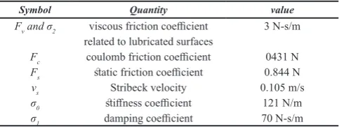
Table 1. Friction Models Paramerets Description

Symbol Quantity value

Fv and σ2

Fc

Fs

vs

σ0

σ1

viscous friction coefficient related to lubricated surfaces

coulomb friction coefficient static friction coefficient

are shown in Fig. 2 and Fig. 3. The nonlinear controller can cope with static models of friction without compensation loop while the linear one is incapable of doing this. The NOC has more robustness to uncertainty in the mass of cart and pendulum than that of the linear controller [24]. In terms of domain of attraction, there is no significant difference and using higher terms in optimal control signal does not necessarily guarantee larger domain of attraction [20]. It is necessary to mention that changing Qand R does not have any significant effect on the performance of the LQR controller [10], [16].

3- 2- Adaptive Anti-Disturbance Technique for Friction Compensation

The designed nonlinear optimal controller is capable of coping with applied friction based on classical and exponential models in some special conditions. The importance of designed controller is the elimination of friction effects for two significant models without using compensator while there are many papers that use linear controller and compensator to eliminate friction effects.

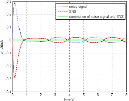
In the case of LuGre model, as it is shown in Fig. 3(c), there is a sinusoid fluctuations around the origin with unknown amplitude, frequency, and phase. In fact, it is supposed that there exists a disturbance sinusoid signal which is added to the system and our aim is constructing a spurious signal with the same amplitude (negative sign), frequency, and phase as a disturbance signal which is added to the main signal. Hence, the spurious and original disturbance signal neutralize each other and the desired behavior is reproduced [16].

The specified disturbance signal is presented as it follows:

(

)

1

sin n

i j j

j

d A ωt ϕ

=

=

∑

+ ₍₁₃₎

where Aj , ωj , and ϕj are unknown amplitude, frequency,

and phase, respectively. With some mathematical manipulation, the relation (13) can be rewritten as [16], [24]:

( )

( )

(

1 2

)

1

sin cos

n

j j j j

j

d α ωt α ωt

=

=

∑

+ ₍₁₄₎

where

( )

( )

1 cos and 2 sin .

j Aj j j Aj j

α = ϕ α = ϕ ₍₁₅₎

In (15), the parameters αj1 and αj2 are unknown. By

obtaining these parameters, Aj and ϕj are estimated by the

following relations.

2

2 2 1

1 2

1

and tan j

j j j j

j

A α α ϕ α

α

−  

= + = _ _

  (16)

The presented format for disturbance signal in (14) is SPM; hence, with the use of gradient algorithm (GA) the unknown parameters αjand ωj can be estimated [25]. We can rewrite

(14) in the following SPM structure.

T

z =θ ψ_, (17)

where z is considered as the estimation of disturbance signal dand _θT _{is a raw vector whose elements consist of}

the unknowns parameters αj1 and αj2 for j =1, , n. The

terms cos

( )

ϕj and sin

( )

ϕj for j =1, , n are elements of

the vector ψ . To use GA, the vector ψ should be known. The unknown frequencies, i.e.ωj, can be estimated using

Fourier transformation of disturbance signal and segregation

Fig. 3. Cart position with initial condition x₀T_{=[0 0.4235 0 0]}

in the presence of friction as disturbance signal under a nonlinear controller; (a) Da Vinci model, (b) Exponential model,

(c) LuGre model.

Fig. 2. Cart position with initial condition x₀T_{=[0 0.2325 0 0]}

in the presence of friction as disturbance signal under a linear controller.

Fig. 1. Comparison between linear and nonlinear optimal controller in the closed loop system with the initial condition

x₀T_{=[0 0.5232 0 0]; (a) cart position, (b) energy of error signal}

dominant Frequencies [16]. Hence, by inserting the frequencies in vector ψ , the elements of the unknown vector

θ are estimated using the following adaptation law,

θ= Γεϕ_, (18)

where _{Γ = Γ >}T 0 _{is the adaptation gain and ε is the} normalized error between estimated and real disturbance signal [25].

Comparison between spurious and original disturbance signal is shown in Fig. 4. Also, the modified cart position after applying friction compensator is plotted in Fig. 5. To obtain the dominant frequencies, we need to conduct an offline experiment without any special conditions, while in some papers, satisfying some special conditions or conducting more than one experiment is necessary [13], [10].

4- Nonlinear Controller Design for Augmented System

with Friction

All the presented friction models have hard nonlinear terms. In this section, friction model is integrated into the system model and, then, a nonlinear optimal controller is designed for the overall system. In optimal controller design procedure for the system x f x =

( )

, at least, the function f x

( )

should belong to the set _C1 _{. Unfortunately, the sign function in (1) and (2)}

and absolute value function in (4) are not differentiable and cannot be linearized. Therefore, three continuous functions are presented to approximate the hard nonlinear terms.

4- 1- Sigmoid Function

The SIPC system has an equilibrium point in the origin and the sign function in (1) and (2) is not differentiable at this point. Hence, by substituting the following function for sign function, we can approximate it.

( )

1 1

ax

ax

e sign x

e −

−

− ≈

+ _, (19)

where a∈

(

0 ∞

)

is an arbitrary parameter and for a→ ∞ we would have a better approximate for the sign function. Now, linearization of the augmented system around the origin can be done and the optimal control problem based on cost function (6) would be nice which makes it possible to design a linear and nonlinear optimal controller for the augmented system. Fig. 6(a) shows the cart position in the closed loop system based on the approximation given in (19).

4- 2- Delta Dirac

The Delta Dirac function is presented as it follows,

( )

2 2

1 x

a

a x e

a

δ

π

  −_ _  

= (20)

where the parameter a is an arbitrary positive number and as

0

a→ , the function δa

( )

x converges into the behavior of

an impulse function. Substituting the Delta Dirac function for the first derivation of sign function makes it possible to design linear and nonlinear optimal controller. The cart position is shown in Fig. 6(b). In the next part, a continuous function is proposed to approximate the absolute value function in LuGre dynamic model.

4- 3- Absolute Value Approximate Function

The absolute value function presented in the state space equation governing LuGre friction model is not differentiable

at the origin. Instead of this function, the following approximation is presented

2

x ≈ x +ε (21)

Where parameterε can have an arbitrarily value on interval

(

0 ∞

)

. For ε →0 the approximate function converges to the original function. As shown in Fig. 7, in this case, using a nonlinear optimal controller contributes into reduction of the amplitude of fluctuations and its frequency significantly. The proposed approximation functions have a significant advantage that is their differentiability around the origin. In the first and second cases, the domain of attraction of closed loop system is compared by simulations. Using sigmoid function leads to the larger domain of attraction, but considering the characteristics of the response, they are similar. In the third case, the amplitude of fluctuations has decreased to 0.008(m) which for the closed loop system without friction compensator is about 0.08 and from the domain of attraction outlook, they are the same. In addition to the mentioned points, there is no need to use state observer and this is another property of the proposed approximation.

Fig. 5. (a) Cart position using friction compensation technique with initial condition x₀T_{=[0 0.3488 0 0] ,}

(b) energy of error signal.

5- Conclusion

Friction is a nonlinear phenomenon and when is modeled comprises the hard-nonlinearities. It has destructive effects on closed loop behavior of the system. The problem of friction compensation was addressed in this paper. Two techniques are proposed. The first presented technique, which is a two-layer approach, consists of a nonlinear optimal controller based on the approximate solution of HJB PDE and an adaptive online friction compensator. The utilized nonlinear controller rather than the simple linear ones which has been used in other papers as a control layer has more advantages in terms of the domain of attraction and robustness. In the second method, friction model was integrated into the system model and a nonlinear optimal controller is designed for the overall system. Because of the non-differentiablity property of hard nonlinearities terms in friction models, we were unable to design linear or nonlinear controllers that work based on the

linearized system. Therefore, some approximate functions were proposed to approximate discontinuous functions and made it possible to design linear and nonlinear controllers such as LQR and nonlinear optimal one (based on HJB PDE). It was shown by simulations that these approximations are effective even in the absence of friction compensator.

References

[1] H.K. Khalil, Nonlinear control, Pearson New York, 2015.

[2] J.-J.E. Slotine, W. Li, Applied nonlinear control, Prentice hall Englewood Cliffs, NJ, 1991.

[3] C.C. De Wit, H. Olsson, K.J. Astrom, P. Lischinsky, A new model for control of systems with friction, IEEE Transactions on automatic control, 40(3) (1995) 419-425.

[4] B. Armstrong-Hélouvry, P. Dupont, C.C. De Wit, A survey of models, analysis tools and compensation methods for the control of machines with friction, Automatica, 30(7) (1994) 1083-1138.

[5] F. Al-Bender, V. Lampaert, J. Swevers, The generalized Maxwell-slip model: a novel model for friction simulation and compensation, IEEE Transactions on automatic control, 50(11) (2005) 1883-1887.

[6] P. Dupont, V. Hayward, B. Armstrong, F. Altpeter, Single state elastoplastic friction models, IEEE Transactions on automatic control, 47(5) (2002) 787-792.

[7] M. Ruderman, T. Bertram, Two-state dynamic friction model with elasto-plasticity, Mechanical Systems and Signal Processing, 39(1-2) (2013) 316-332.

[8] H. Olsson, Control systems with friction,1997.

[9] S.A. Campbell, S. Crawford, K. Morris, Friction and the inverted pendulum stabilization problem, Journal of Dynamic Systems, Measurement, and Control, 130(5) (2008) 054502.

[10] M. Ruderman, T. Bertram, Two-state dynamic friction

model with elasto-plasticity, Mechanical Systems and Signal Processing, 39(1-2) (2013) 316-332.

[11] C.C. De Wit, P. Lischinsky, Adaptive friction

compensation with partially known dynamic friction model, International journal of adaptive control and signal processing, 11(1) (1997) 65-80.

[12] D.D. Rizos, S.D. Fassois, Friction identification

based upon the LuGre and Maxwell slip models, IEEE Transactions on Control Systems Technology, 17(1) (2009) 153-160.

[13] R.H. Hensen, M.J. van de Molengraft, M. Steinbuch,

Frequency domain identification of dynamic friction model parameters, IEEE Transactions on Control Systems Technology, 10(2) (2002) 191-196.

[14] L. Freidovich, A. Robertsson, A. Shiriaev, R. Johansson, LuGre-model-based friction compensation, IEEE Transactions on Control Systems Technology, 18(1) (2010) 194-200.

[15] A. Amthor, S. Zschaeck, C. Ament, High precision

position control using an adaptive friction compensation approach, IEEE Transactions on automatic control, 55(1) (2010) 274-278.

[16] M.N. Monfared, M.J. Yazdanpanah, Adaptive

compensation technique for nonlinear dynamic and static models of friction, in: 2015 23rd Iranian Conference on Electrical Engineering, IEEE, 2015, pp. 988-993.

Fig. 7. Cart position response to initial condition

x₀T_{=[0 0.27 0 0] in closed loop with optimal controller for the}

augmented system with dynamic friction. The blue one is related to the closed loop system without friction compensator and the

red one is related to the closed loop augmented system. Fig. 6. Cart position with initial condition x₀T_{=[0 0.08 0 0] in}

closed loop with the optimal controller for the augmented system with classic friction (Red: nonlinear controller, blue: Linear

[17] C. Makkar, G. Hu, W.G. Sawyer, W.E. Dixon, Lyapunov-based tracking control in the presence of uncertain nonlinear parameterizable friction, IEEE Transactions on Automatic Control, 52(10) (2007) 1988-1994.

[18] D.E. Kirk, Optimal control theory: an introduction,

Courier Corporation, 2012.

[19] C.L. Navasca, A.J. Krener, Solution of hamilton

jacobi bellman equations, in: Proceedings of the 39th IEEE Conference on Decision and Control (Cat. No. 00CH37187), IEEE, 2000, pp. 570-574.

[20] T. Hunt, A.J. Krener, Improved patchy solution to the Hamilton-Jacobi-Bellman equations, in: 49th IEEE Conference on Decision and Control (CDC), IEEE, 2010, pp. 5835-5839.

[21] R.M. Milasi, M.J. Yazdanpanah, C. Lucas, Nonlinear

optimal control of washing machine based on approximate solution of HJB equation, Optimal Control Applications and Methods, 29(1) (2008) 1-18.

[22] M.N. Monfared, M.H. Dolatabadi, A. Fakharian,

Nonlinear optimal control of magnetic levitation system based on HJB equation approximate solution, in: 2014 22nd Iranian Conference on Electrical Engineering (ICEE), IEEE, 2014, pp. 1360-1365.

[23] R.W. Beard, G.N. Saridis, J.T. Wen, Galerkin

approximations of the generalized Hamilton-Jacobi-Bellman equation, Automatica, 33(12) (1997) 2159-2177.

[24] M. Nazari Monfared, M. Yazdanpanah, Friction

Compensation for Dynamic and Static Models Using Nonlinear Adaptive Optimal Technique, AUT Journal of Modeling and Simulation, 46(1) (2014) 1-10.

[25] P. Ioannou, B. Fidan, Adaptive control tutorial, Society for Industrial and Applied Mathematics, in, SIAM books Philadelphia, 2006.

[26] H. Olsson, K.J. Åström, C.C. De Wit, M. Gäfvert, P.

Lischinsky, Friction models and friction compensation,

Eur. J. Control, 4(3) (1998) 176-195.

[27] F. Marques, P. Flores, J.P. Claro, H.M. Lankarani, A

survey and comparison of several friction force models for dynamic analysis of multibody mechanical systems, Nonlinear Dynamics, 86(3) (2016) 1407-1443.

[28] E. Pennestrì, V. Rossi, P. Salvini, P.P. Valentini, Review and comparison of dry friction force models, Nonlinear dynamics, 83(4) (2016) 1785-1801.

[29] A.K. Padthe, B. Drincic, J. Oh, D.D. Rizos, S.D.

Fassois, D.S. Bernstein, Duhem modeling of friction-induced hysteresis, IEEE Control Systems Magazine, 28(5) (2008) 90-107.

[30] P.-A. Bliman, Mathematical study of the Dahl’s friction model, European journal of mechanics. A. Solids, 11(6) (1992) 835-848.

[31] R. Hensen, M. van de Molengraft, M. Steinbuch,

Friction induced limit cycling: Hunting, Automatica, 39(12) (2003) 2131-2137.

[32] B. Bukkems, Friction induced limit cycling: an

experimental case study, DCT rapporten, 2001 (2001).

[33] N. Van De Wouw, R. Leine, Robust impulsive control

of motion systems with uncertain friction, International Journal of Robust and Nonlinear Control, 22(4) (2012) 369-397.

[34] L. Márton, B. Lantos, Control of mechanical systems

with Stribeck friction and backlash, Systems & Control Letters, 58(2) (2009) 141-147.

[35] B. Liu, S. Nie, Dynamic Parameters Identification of

LuGre Friction Model Based on Chain Code Technique, in: Proceedings of the 14th IFToMM World Congress,

國立臺灣大學機械系, 2015, pp. 216-222.

[36] A. Nejadfard, M.J. Yazdanpanah, I. Hassanzadeh,

Friction compensation of double inverted pendulum on a cart using locally linear neuro-fuzzy model, Neural Computing and Applications, 22(2) (2013) 337-347.

Pleasecitethisarticleusing:

M. Nazari-Monfared and M. J. Yazdanpanah, Elimination of Hard-Nonlinearities Destructive Effects in Control Systems Using Approximate Techniques, AUT J. Model. Simul., 50(2) (2018) 117-122.