Lane Change Trajectory Model Considering the Driver Effects Based on MANFIS

(1)

International Journal of Automotive Engineering Vol. 2, Number 4, Oct 2012

Lane Change Trajectory Model Considering the Driver

Effects Based on MANFIS

A.Ghaffari1, A. Khodayari2*, S. Arvin3, F. Alimardani4 1

Professor, 2 PhD, Mechanical Engineering Department, K. N. Toosi University of Technology, Tehran, Iran.

3

M.Sc. Mechanical Engineering Department, Islamic Azad University, South Branch, Tehran, Iran.

4

M.Sc. Mechatronics Engineering Department, K. N. Toosi University of Technology, Tehran, Iran.

[email protected]

Abstract

The lane change maneuver is among the most popular driving behaviors. It is also the basic element of important maneuvers like overtaking maneuver. Therefore, it is chosen as the focus of this study and novel multi-input multi-output adaptive neuro-fuzzy inference system models (MANFIS) are proposed for this behavior. These models are able to simulate and predict the future behavior of a Driver-Vehicle-Unit in the lane change maneuver for various time delays. To design these models, the lane change maneuvers are extracted from the real traffic datasets. But, before extracting these maneuvers, several conditions are defined which assure the extraction of only those lane change maneuvers that have a smooth and uniform trajectory. Using the field data, the outputs of the MANFIS models are validated and compared with the real traffic data. In addition, the result of these models is compared with the result of other trajectory models. This comparison provides a better chance to analyze the performance of these models. The simulation results show that these models have a very close compatibility with the field data and reflect the situation of the traffic flow in a more realistic way.

Keywords: Intelligent Transportation Systems, lane change maneuver, modeling, multi-output ANFIS..

1. Introduction

Nowadays, intelligent transportation systems (ITS) play an important role in transportation industry. The prominent aspect of these systems is their ability to increase safety and improve the traffic flow [1-2]. ITS achieves these goals by incorporating up-to-date information technologies of all kinds in the transportation field [3]. One of the concerns of ITS is microscopic models of traffic flow, and specially, models of different driving maneuvers such as car following and lane change behavior. In these maneuvers, the behavior of each driver is different from the behavior of others since each driver follows his own specific patterns during driving. Many Driver

Assistant Systems (DAS) require a model

representing the typical driving patterns of the target driver in order to cooperate in the driving behavior. Driver Models can be trained either in offline or online manners [3, 4]. Lane change models are among the most important microscopic traffic flow models. The object of these models is to obtain desired

behavior of a Driver-Vehicle-Unit (DVU) in the lane change maneuver. Fig. 1 shows a typical situation of a lane change maneuver. When the necessity to change the current lane arises, the distances between the main vehicle and other vehicles should be checked before any decision making. If the distances were safe enough to prevent accidents, the lane change maneuver can get started. To perform the maneuver, the vehicle initiates to move to the adjacent lane. By starting to move to the left lane, the heading angle of the vehicle begins to increase until the vehicle gets to the middle of the left lane. At this point, the maneuver is completed and the vehicle can arrange to move in the straight path again. As a result, the heading angle begins to decrease [5].

Humans play an inevitable role in the operation and control of human-machine systems. A Driver-Vehicle Unit is an example of such systems. With

advances in emerging vehicle-based ITS

technologies, it becomes even more important to understand the normative behavior response of drivers and changes under new systems [2]. Based on Rasmussen’s human-machine model, shown in Fig. 2

(2)

A.Ghaffari, A. Khodayari, S. Arvin and F. Alimardani 262

International Journal of Automotive Engineering Vol. 2, Number 4, Oct 2012

Fig1.Lane change behavior [5].

Fig2.Rasmussen’s human-machine model [6].

[6], driver behavior can also be separated into a hierarchical structure with three levels: the strategic

Tactical and operational level. At the highest level (strategic), goals of each driver are determined, and a route is planned based on these goals. The lowest operational level reflects the real actions of drivers, e.g., steering, pressing pedal, and gearing. In the middle level, certain maneuvers are selected to achieve short-term objectives, e.g., interactions with other road users and road infrastructures.

In this paper, new multi-output ANFIS (MANFIS) models for lane change maneuver are proposed. These models are able to predict the future behavior of a lane change maneuver for three different delay times. 0.1s, 0.2s and 0.3s are these constant delay times

2. Brief Review on The Lane Change Models

To develop microscopic traffic simulation of high fidelity, researchers are often interested in imitating human’s real driving behavior at a tactical level. That is, without describing the detailed driver actions, DVUs in the simulation are modeled to replicate their states in reality, i.e., the profiles of vehicle position, velocity, acceleration, and steering angle. Fig. 3 shows the model structure of a DVU in which the detailed driver actions become internal [7]

So far, various models for lane change maneuver have been presented [8-9]. Seimenis and Fotiades presented a mathematical lane change model by using Clothoidal Theory and Bezier Points. In this study, the lane change trajectory points were approximated using a polynomial which was called s-series. This model could change curvature radius during lane

(3)

263 Lane Change Trajectory Model Considering the…

International Journal of Automotive Engineering Vol. 2, Number4, Oct 2012

change path regularly using continuous monitoring of centrifugal acceleration through velocity control [10]. Hsu and Liu presented a lane change model for platoon maneuvers in highways. In this study, first the required equations to model the lane change maneuver were obtained using two robots, and then the model was generalized for the vehicle [11]. Toledo-Moreo and Zamora-Izquierdo presented a lane change prediction model for collision avoidance in highways using interactive multiple models (IMM) method. This model predicted the positioning using the extended Kalman filters (EKFs) that was run by an IMM-based algorithm [12]. Dogan et al. presented a neural network model for lane change maneuver. This model had a memory part that activations of neurons in each step are stored in this part for using in the next steps. In this model, back propagation algorithm was used, and the data related to real experiments were used for training [13]. Alonso et al. applied image processing method to develop a lane change model, based on motion-driven vehicle tracking and monitoring the rear view mirror of vehicle. In this paper, first, the optical flow in real time was computed using a digital signal processor (DSP). Then, the position of the lane change trajectory points were computed using a standard processor [14]. Ahle and Soffker presented a lane change model based on the relationships governing the parameters and situations of the operator. In this study, first, various situations of the vehicle and actions of operators (mean braking, driving and lane changing) were defined. Then, a lane change algorithm base on situation-operator mode1 (SOM) was presented [15]. Liu et al. applied Parallel Bayesian Networks (PBN) to develop a lane change model. The basic operation of this model was the analysis of the steering angles and their difference [16]. The final status of driver behavior was determined using the largest probability of each status during the lane change. Then, the presented model

was compared by Gussian Bayesian Network (GBN). GBN is a method for estimation of the driver's behavior state using steering angle in one period. Comparing these models showed that the PBN model had less error and can decrease response time of the behavior state judgment during lane change [17]. Wakasugi presented a model to alarm the appropriate time for lane change, based on the relationship between lane-change tasks and closing vehicles in the passing lane. In this paper, simulation was done by a linear prediction model, using the data related to real experiments [18]. Shamir offered an optimal lane-change trajectory to be used under normal conditions for overtaking maneuvers. To suggest a trajectory for a lane change, he considered phase 3 of an overtaking lane for convenience. To determine the trajectory for lane change maneuver, a polynomial expression was fitted for x(t) and y(t). By writing down a general fifth-degree polynomial, the equations for coordinate x and y of the trajectory were obtained [19].

As mentioned above, various studies have been done on lane changing models. In this study, a new model will be proposed which improve different aspects of the available models. Artificial neural networks are favorable tools providing the possibility of exploiting real observed data while developing the models. In addition, fuzzy logic can be a potential method to deal with structural and parametric uncertainties for non-linear behaviors. Neuro-fuzzy models, such as ANFIS, are combinations of artificial neural networks and fuzzy inference systems, therefore these models have advantages of both methods. Integration of human expert knowledge expressed by linguistic variables, and learning based on the data are powerful tools enabling neuro-fuzzy models to deal with uncertainties and inaccuracies [20]. Since lane change is a highly non-linear behavior, ANFIS is a powerful tool to model the lane change maneuver. In the next part, the design of the ANFIS lane change model is described

Fig3.Structure of a DVU model [2].

3. ANFIS Lane Change Models Design Since ANFIS is the basis of this design, this

section starts with a brief review on ANFIS and then

(4)

multi-output ANFIS (MANFIS) structure is

expressed. Next, the database used for the design of the model is explained briefly. In order to have a smooth lane change trajectory, some conditions are defined and the lane change data are extracted according to these conditions. At the end of this section, the structure of the models is described.

A. ANFIS Architecture

Since in this research, ANIS type-3 is used to model the lane change behavior, the ANFIS structure is briefly explained in this section. Detailed information about ANFIS is available in [21]. ANFIS is a system which has the ability to make human-like decisions. Since ANFIS structure is composed of the combination of neural network and fuzzy logic, using ANFIS for non-liner systems will have appropriate result [22]. The if–then fuzzy rules that are used in ANFIS are Takagi-Sugeno’s type, and a recursive least square (RLS) is the basis of learning procedure. ANFIS architecture (type-3 ANFIS) is shown in Fig. 4. The structure is composed of 5 layers, that each layer has one or several nodes. There are two types of nodes: square node (adaptive node) and circle node (fixed node) [23].

In these equations x and y are inputs to node i, andai, i

b _and c_i_{are parameters of the membership}

functions, andpi_,qi_andri_{are parameters set of the} fuzzy rules. (Defining µ Bi(y) is similar to the process of defining µ Ai(x) . The only difference is that y is used instead of x).

Fig4.ANFIS architecture (type-3 ANFIS) [23].

ANFIS has a major constraint which is its single output structure. To solve this problem, multi-output model can be made by connecting several single output models. In other words, putting as many ANFIS models side by side, as there are required outputs is an approach of having multiple outputs. The architecture of a two-output MANFIS model is shown in Fig. 5 [24].

Besides the advantages of ANFIS, MANFIS has several other privileges. MANFIS needs fewer numbers of training to get the same error of single ANFIS. Therefore, faster and simpler results can be obtained based on MANFIS. In this study, MANFIS is used to effectively predict the future behavior of a lane change maneuver [25].

B. Datasets

Real overtaking data from US Federal Highway Administration’s NGSIM dataset is used to train the MANFIS prediction models [26]. The NGSIM datasets represent the most detailed and accurate field data collected to date for traffic micro simulation research and development. In June 2005, a dataset of trajectory data of vehicles travelling during the

The first layer is consisted of square nodes, and the value of the input membership functions ( ( )

i

A x

µ _{) are computed in this layer. Usually we}

choose ( ) i

A x

µ

to be bell-shaped such as equations (1) and (2). The second layer is made of circle nodes. Output of each node in this layer represents the firing strength of a rule (wi). This value is

computed by equation (3). The third layer is made of circle nodes. In this layer, the ratio of the each rule's firing strength to the sum of all rules firing strengths (wi) is computed through equation (4).

The fourth layer is consisted of square nodes, and executes the part of fuzzy rules by equation (5). Finally the single node in the fifth layer, which is a circle node, computes the output system using the summation of all incoming signals and is calculated by equation (6).

2

1 ( )

1 [ ( ) ]

i i A b i i x x c a µ = − + (1) 2

( ) e x p { ( ) }

i i A i x c x a

µ = − − (2)

( ) ( ), 1, 2

i i

i A B

w = µ x ×µ y i = (3)

1 2

, 1, 2

i i w w i w w = = + (4)

i i i i

f = p x+q y+r (5)

_ i i i

i i

i

i _i

w f

o v e r a l l o u tp u t w f

w

=

∑

=

∑

(6)

(5)

morning peak period on a segment of Interstate 101 highway in Emeryville (San Francisco), California has been made using eight cameras on top of the 154m tall 10 Universal City Plaza next to the Hollywood Freeway US-101. On a road section of 640m, 6101 vehicle trajectories have been recorded in three consecutive 15-minute intervals. This dataset has been published as the US-101 Dataset. The dataset consists of detailed vehicle trajectory data on a merge section of eastbound US-101, as shown in Fig. 6. The data is collected in 0.1 second intervals. Any measured sample in this dataset has 18 features of each driver-vehicle unit in any sample time, such as longitudinal and lateral position, velocity, acceleration, time, number of road, vehicle class, front vehicle and etc [27].

The other dataset was published as the I-80 Dataset. Researchers for the NGSIM program collected detailed vehicle trajectory data on eastbound

I-80 in the San Francisco Bay area in Emeryville, CA, as shown in Fig. 7, on April 13, 2005. The study area was approximately 500 meters (1,640 feet) in length and consisted of six freeway lanes, including a high-occupancy vehicle (HOV) lane. An onramp also was located within the study area. Seven synchronized digital video cameras, mounted from the top of a 30-story building adjacent to the freeway, recorded vehicles passing through the study area. This vehicle trajectory data provided the precise location of each vehicle within the study area every one-tenth of a second, resulting in detailed lane positions and locations relative to other vehicles. A total of 45 minutes of data are available in the full dataset, segmented into three 15-minute periods. These periods represent the buildup of congestion, or the transition between uncongested and congested conditions, and full congestion during the peak period [28].

Fig5.A two-output MANFIS structure [24]

Fig6.A segment of Interstate 101 highway in Emeryville, San Francisco, California [27]

(6)

Fig7.A segment of eastbound I-80 in the San Francisco Bay area in Emeryville, California [28].

(a) (b)

Fig8.. Comparison of filtered and unfiltered data: (a) acceleration, (b) heading angle.

The data extracted from the datasets, seem to be unfiltered and exhibit some noise artifacts, so these data must be filtered like [29, 30]. A moving average filter has been designed and applied to all data before any further data analysis. Comparison of the unfiltered and filtered data of the acceleration and heading angle of the overtaking vehicle are shown in Fig. 8.

C. .Data Extraction Conditions

In general, there is no certain rule to determine an appropriate lane change maneuver from others. Here, some innovative conditions are determined to help extract the lane change behaviors which have an appropriate trajectory. These conditions are obtained

by analyzing the data related to a DVU behavior in the lane change maneuver. These conditions must be satisfied to provide the safety and convenience of the vehicle's passengers and the vehicle will have a smooth and uniform trajectory [5]. These conditions are explained here.

In order to create a symmetric path for lane change, the vehicle must have passed half of the width and length of the lane change path when half of the time of the maneuver is passed.

Although there is no rule to determine a maximum limit for the heading angle of the vehicle's movement, in order to have an appropriate trajectory, it is better to determine such a limit for the maximum heading angle during the lane change maneuver.

1 2 3 4

-1 0 1 2 3

time(s)

ac

ce

le

ra

ti

o

n

(m

/s

2 )

real filtered

1 2 3 4

-6 -5 -4 -3 -2 -1 0

time(s)

an

g

le

(d

eg

)

real filtered

(7)

Another necessary condition to have a symmetric trajectory is that the sign of heading angle changes only one time in the whole path.

Another condition is that the heading angle does not have sudden changes. Notice that the heading angle does not necessarily changes in all the time steps of the maneuver.

Investigating the data of the appropriate maneuvers shows that the major changes of the heading angle occur at the initial and final time steps of the lane change maneuver. Knowing the maximum

value of the heading angle (ϕMAX _{), the maximum}

changes of the heading angle at each time step can be determined through equation (7).

The next step is to decrease the chance of the vehicle's slip during the lane change maneuver. To do this, first, the free diagram of the vehicle is drawn simply.

This diagram is shown in Fig. 9. Using the Newton's equations, as shown in equations (8) and (9), F1 and F2 are obtained by solving the equations (10) and (11).

where m is the mass of vehicle, I is the inertia moment, c and b are the distances from the center of mass to the front and rear tires, M is the torque of the vehicle, a and v are the vehicle's acceleration and velocity, F1 and F2 are the lateral forces of the front and rear tires, and R is the radius of the curve of the path.

So the maximum limit of F1 and F2 are calculated using equations (12) and (13) by exerting a safety coefficient (fn) to cover the imperfection resulted by approximation.

Which,

Where s1 and s2 are fractions of vehicle weight on the front and rear tires, g is the acceleration of gravity

and µ is the friction coefficient between tiers and the

ground.

In this stage, if F1 and F2 are less than their maximum values, then the velocity and acceleration of the vehicle has the appropriate value for the vehicle not to slip. But if F1 or F2 has a velue more than its maximum one, this condition cannot be satisfied.

The last condition for data separation is about the changes that velocity and acceleration have during the maneuver. Since velocity is a function of acceleration, and the changes of acceleration determines the value of the changes of velocity, it is enough to determine a condition for the rhythm of acceleration changes so that it does not cause sudden movements.

A desired lane change maneuver, is a maneuver which satisfies all the above conditions.

An example of a desired lane change trajectory is shown in Fig .10. As it is shown, the trajectory is smooth and doesn’t have a sudden change.

Fig9.Free diagram of the vehicle in the lane change path [5].

D. Structure of the Models

After extracting the desired lane change data, MANFIS models are designed to predict the 5

MA X M A X

ϕ ϕ

∆ = ± (7)

2 n

v

F m

R =

∑

(8)

a

M I

R =

∑

(9)

2

1 2

2(F F ) mv

R

+ = (10)

2 1

2(b F c F) I a

R

× − × = (11)

1

2

M

n

s mg

F

f

µ

× ×

= (12)

2

M

n

s mg

F

f

µ

× ×

= (13)

1 2, 1 2 1

s >s s +s = (14)

(8)

275

acceleration and heading angle of the vehicle which performs a lane change maneuver. From the extracted data, 75% of the lane change maneuvers are randomly selected to train the model.

The remaining data is set aside for model validation. In this study, three MANFIS models are designed to redict the future behavior of a lane change maneuver. Each of these models has five inputs and two outputs.

The inputs and outputs for all of the models are the same. Inputs of these models are velocity,

acceleration, jerk, heading angle and heading angle rate, and outputs of these models are the acceleration and heading angle. The structure of all three models is similar.

Fig. 11 shows the structure of the MANFIS models. Hybrid algorithm was used to train these models. Each of these models have 162 fuzzy if–then rules of Takagi-Sugeno’s type [31], and each input has three triangular membership functions.

Fig10. Sample of a desired lane change path

Fig11. Structure of all three MANFIS models.

4. Discussion and Results

In this section, in order to validate the performance of the MANFIS models, the behavior of several test vehicles is investigated. In Fig. 12 and Fig. 13, the acceleration and heading angle resulted

by the three MANFIS models are compared with the real data of the first test sample vehicle (LC1). As it is obvious, in part (a) of the figures, which is for the model with 0.1s delay, the results of the models have a very close compatibility with the real data. As the delay time increases, as shown in part (b) and (c), the error increases for both model outputs.

3 4 5 6

590 595 600 605

y(m)

x

(m

)

(9)

To examine the performance of the developed models, various criteria are used to calculate error values. Root mean square error (RMSE) criterion, according to equation (15), is one of the well-known standard errors, and is used as a criterion to compare error aspects in various models. Mean Absolute Error (MAE), according to equation (16), shows how much the predicted results conform to reality [32]. As it is clear from its name, this value is a mean absolute error.

Normalized mean square error (NMSE), according to equation (17), is a method to calculate a standard error in estimating methods that shows the normal difference of real data from the estimated data.

Where, N is the number of test observation, xi shows the real value of the variable being modeled (observed data), ,-_. shows the real value of variable

modeled by the model, and ,̅ is the real mean value

of the variable. Errors in modeling the acceleration and heading angle for all the three MANFIS models,

(a) (b) (c)

Fig12. Acceleration outputs of the three MANFIS models for the first test sample vehicle (LC1): (a) 0.1s delay time, (b) 0.2s delay time,

(c) 0.3s delay time.

Fig13. The heading angle output of the three MANFIS models for the first test sample vehicle (LC1): (a) 0.1s delay time, (b) 0.2s delay

time, (c) 0.3s delay time.

1 2 3 4

-1 -0.5 0 0.5 1 1.5 2 2.5 time(s) ac c el er a to in (m /s 2) test chart real model

1 2 3 4

-2 -1 0 1 2 3 time(s) ac ce le ra ti o n (m /s 2) real model

1 2 3 4

-1.5 -1 -0.5 0 0.5 1 1.5 2 2.5 time(s) ac ce le ra ti o n (m /s 2) real model

1 2 3 4

-5 -4 -3 -2 -1 0 time(s) an g le (d eg ) real model

1 2 3 4

-5 -4 -3 -2 -1 0 time(s) an g le (d e g ) real model

1 2 3 4

-6 -5 -4 -3 -2 -1 0 1 time(s) a n g le (d e g ) real model 2 1 1 ( ) N i i i

RMSE x x

N ₌ =

∑

− ) (15) 1 1 N i i i

MAE x x

N ₌

=

∑

) −

(16)

2 2 2

1 1

[ ( ) ] / [ ( ) ]

N N

i i i

i i

R x x x x

= =

=

∑

−)

∑

−

(17)

(10)

Table I. Result of Error for MANFIS Models: Acceleration

Model Test vehicle RMSE MAE NMSE

0.1s delay time

LC2 0.0842 0.0565 0.0344

LC3 0.1686 0.1126 0.1239

LC4 0.1131 0.0773 0.0673

0.2s delay time

LC2 0.2977 0.1583 0.1793

LC3 0.3381 0.2404 0.2543

LC4 0.2489 0.1775 0.2206

0.3s delay time

LC2 0.4535 0.2529 0.3084

LC3 0.4973 0.3730 0.3559

LC4 0.3549 0.2317 0.2879

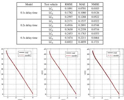
Table 2.Result of Error for MANFIS Models: Heading Angle.

Model Test vehicle RMSE MAE NMSE

0.1s delay time

LC2 0.1091 0.0701 0.0103

LC3 0.1782 0.1080 0.0126

LC4 0.2597 0.1288 0.0522

0.2s delay time

LC2 0.2171 0.1537 0.0322

LC3 0.4916 0.2891 0.0748

LC4 0.3630 0.2358 0.0716

0.3s delay time

LC2 0.2453 0.1763 0.0353

LC3 0.3474 0.2211 0.0464

LC4 0.6922 0.4859 0.1721

Fig14. Comparison of the trajectory of the three MANFIS models with real trajectory for the first test vehicle (LC1): (a) model by 0.1s

delay time, (b) model by 0.2s delay time, (c) model by 0.3s delay time.

Considering these criteria are summarized in Table I and Table II. The results for only three test vehicles are shown in these tables.

Using the acceleration and heading angle resulted by the models, the coordinates of the trajectory for each test vehicle can be calculated. This trajectory can

be compared by the real trajectory. In Fig. 14, the real trajectory and the trajectory resulted from the models are shown for the first test vehicle (LC1).

To examine the performance of the developed models, various error criteria are used. But since the total time of the trajectory of the optimal model is not

(11)

equal to the time in real trajectory data, it is not possible to calculate these criteria for this model. So, the results of these criteria are only calculated for the MANFIS model.

The absolute horizontal transport deviation (AHTD), according to equation (18), shows the mean deviation between a modeled trajectory and the corresponding true trajectory. The trajectory based on field data is considered as true trajectory. Another useful statistical concept is the mean relative horizontal deviation (RHTD), according to equation (20).

This is defined as the ratio between the absolute transport deviation and the mean total travel distance of the true trajectory (L₅(t)), according to equation (12).

In these equations, X₇(t) and x₇(t), respectively, show the real and model value of the coordinate x. In addition, Y₇(t) and y₇(t) show the real and model value of the coordinate y. N is the number of test observations at travel time t [33, 34].

( ) 100

( ) H

AHTD RHTD t

L t

= ×

(19)

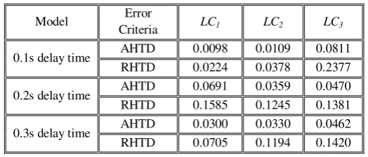
Errors between the real trajectory and the trajectory resulted by the three models, considering these criteria are summarized in Table 3.

In this section, the lane change trajectory of the first MANFIS model will be compared with the trajectory of the optimal trajectory model presented by Shamir in 2004 [19]. In the optimal trajectory model, Shamir assumed that the lateral displacement is always equal to the width of the lane (W). Notice that the MANFIS model and the optimal model present the lateral and longitudinal coordinates with unlike parameters. In the MANFIS model, lateral coordinate is shown by x and the longitudinal coordinate is shown by y. But in the optimal model, the names of the parameters are vice versa. For the same test vehicle, the optimal trajectory model offers the trajectory shown in Fig. 15 (a).

Table 3. Trajectories error for three examined samples.

Model Error

Criteria LC1 LC2 LC3

0.1s delay time AHTD 0.0098 0.0109 0.0811

RHTD 0.0224 0.0378 0.2377

0.2s delay time AHTD 0.0691 0.0359 0.0470

RHTD 0.1585 0.1245 0.1381

0.3s delay time AHTD 0.0300 0.0330 0.0462

RHTD 0.0705 0.1194 0.1420

One disadvantage of the optimal model is that the lateral distance traveled is always equal to the width of the road (W). But in reality, it does not happen as ideal as the optimal model shows. Therefore, the trajectory of the first phase always starts from a point with negative coordinate x. All the trajectories resulted by this model have this property. Because of this property, the start and final points of the trajectory are not even close to reality. In addition, the optimal model is not able to predict the trajectory for test vehicles with negative or zero acceleration, but the MANFIS model is completely capable of predicting the trajectory for different values of the

acceleration. Also, for cases with positive

acceleration, the model does not have a proper result when the value of the acceleration increases. An example of this case is shown in Fig. 15 (b). In these

situations, the trajectory for the lane change phases of the maneuver will not be a smooth trajectory anymore. Another problem is that in the optimal model, the total time of the maneuver is not equal to the time spent in reality. One more disadvantage is about the total distance traveled during the maneuver. The optimal model isn’t able to predict the total distance correctly. So, in some cases the distance is more than the real distance, and sometimes it is less. Here, in order to have a better comparison between the trajectories of the two models, the trajectory of the optimal model is rotated. Then, it is shifted to the start point of the real trajectory. After rotation, in both trajectories, the horizontal axis shows the lateral displacement, and the vertical axis shows the longitudinal displacement. The comparison of the output of the two models with real data for the first test vehicle is shown in Fig. 16 (a). Also, in Fig .16

[ ]2 [ ]2 1

2 1

1

( ) { ( ) ( ) ( ) ( ) }

N

n n n n

n

AHTD t X t x t Y t y t

N =

=

∑

− + −

(18)

(12)

(b), lane change trajectory of the MANFIS model and optimal model are compared with lane change trajectory of the real data for the second sample (LC2). For this case, the acceleration of the test

vehicle was more than the previous case. As it is shown, the trajectory of the lane change phases is not a uniform trajectory.

(a)

(b)

Fig15. . The optimal trajectory model: (a) Sample of a smooth trajectory, (b) Sample of an undesired trajectory.

-200 -150 -100 -50

0 1 2 3 4

trajectory of the whole maneuver

X (m)

Y

(

m

)

Optimal Model

-200 -150 -100 -50 0

0 1 2 3 4

trajectory of the whole maneuver

X (m)

Y

(

m

)

Optimal Model

(13)

5. Conclusion

In this study, three MANFIS models have been presented for the prediction of the vehicle which performs a lane change maneuver. These models have been designed to predict the lane change parameters with 0.1s, 0.2s and 0.3s delay times, respectively. The inputs of these MANFIS models were velocity, acceleration, jerk, heading angle, and heading angle rate, and its outputs were acceleration and healing angle. Since DVU behavior data have been used in the designing MANFIS models, the obtained results are very close to what happens in reality. To design these models, a wide range of the data of the lane change maneuvers is used and in order to decrease the noise and artifacts of the data, they are filtered with the moving average filter. Also, in order to increase the safety and comfort of the passengers, using the defined conditions, appropriate data for modeling are extracted from the NGSIM datasets. The testing results show that MANFIS models have low error and high precision and can predict the lane change trajectory with high accordance with the actual lane change trajectory. But by increasing the delay time, the models precision decreases. So, the first model can predict the lane change maneuver with higher precision in comparison with the second and third models, and consequently, the precision of the second model is more than the precision of the third model. Also, the performance of the first model was compared with the result of the optimal trajectory model presented by Shamir in 2004. Comparison

shows that the optimal trajectory model does not offer a proper trajectory, but the MANFIS model is very accordant with the real data. As a whole, the error tables and the figures show that these MANFIS models have a strong capability with real data in comparison with other presented models.

6. Acknowledgement

The authors would like to state their appreciation to US Federal Highway Administration and Next Generation SIMulation (NGSIM) for providing the datasets used in this paper.

REFERENCES

[1]. A. Khodayari, A. Ghaffari, R. Kazemi, N.

Manavizadeh,“ANFIS Based Modeling and Prediction Car Following Behavior in Real Traffic Flow Based on Instantaneous Reaction Delay”, 13th International IEEE Annual

Conference on Intelligent Transportation

Systems, Madeira Island, Portugal, September 19-22, 2010.

[2]. X. Ma, I. Andréasson, “Behavior Measurement,

Analysis, and Regime Classification in Car Following”, IEEE Transactions on Intelligent Transportation Systems, vol. 8, no. 1,pp. 144-156, 2007.

[3]. A. Khodayari, R. Kazemi, A. Ghaffari, R.

Braunstingl, “Design of an Improved Fuzzy Logic Based Model for Prediction of Car Following Behavior” , IEEE Intemational

(a) (b)

Fig16. Comparing the trajectory of the MANFIS model and optimal model with the real trajectory: (a) for first sample (LC1), (b) for second sample (LC2).

(14)

Conference on Mechatronics, April 13-15, 2011, Istanbul, Turkey

[4]. C. Miyajima, Y. Nishiwaki, K. Ozawa, T.

Wakita, K. Itou, K. Takeda,and F. Itakura, “Driver Modeling Based on Driving Behavior and ItsEvaluation in Driver Identification”, Proceedings of the IEEE, Vol.95, No.2, 2007.

[5]. A. Ghaffari, A. Khodayari, S. Arvin, “ANFIS

Based Modeling and Prediction Lane Change Behavior in Real Traffic Flow”, IEEE

International Conference on Intelligent

Computing and Intelligent Systems (ICIS 2011), China, 2011.

[6]. J. Rasmussen, “Information Processing and

Human.Machine Interaction: An Approach to Cognitive Engineering”, New York: Elsevier, 1986.

[7]. A. Khodayari, A. Ghaffari, R. Kazemi, R.

Braunstingl, “Modify Car Following Model by Human Effects Based on Locally Linear Neuro Fuzzy”, IEEE Intelligent Vehicles Symposium (IV), Baden-Baden, Germany ,June 5-9, 2011.

[8]. J. Feng , J. Ruan , Y. Li , “Study on Intelligent

Vehicle Lane Change Path Planning and Control Simulation” , Proceedings of the IEEE

International Conference on Information

Acquisition August 20 - 23, 2006, Weihai, Shandong, China.

[9]. R. Schubert, K. Schulze, G. Wanielik,

“Situation Assessment for Automatic Lane-Change Maneuvers” , IEEE Transactions on Intelligent Transportation Systems, Vol. 11, N0. 3, September 2010.

[10].J. Seimenis , K. Fotiades , “Fast Lane Changing

Algorithm for Intelligent Vehicle Highway Systems Using Clothoidal Theory and Bezier Points” , IEEE, Proceedings of the Intelligent Vehicles Symposium 2005, pp. 73-77.

[11].H. C. a-Hung Hsu, A. Liu, “Platoon Lane

Change Maneuvers for Automated Highway Systems” , Proceedings of the IEEE Conference on Robotics, Automation and Mechatronics Singapore, 1-3 December, 2004.

[12].R. Toledo-Moreo, M. A. Zamora-Izquierdo,

“IMM-Based Lane-Change Prediction in

Highways With Low-Cost GPS/INS” , IEEE Transactions on Intelligent Transportation Systems, Vol. 10, No. 1, March 2009.

[13].U. Dogan , H. Edelbrunner , I. Iossifidis ,

“Towards a Driver Model: Preliminary Study of Lane Change Behavior” , Proceedings of the

11th International IEEE Conference on

Intelligent Transportation Systems Beijing, China, October 12-15, 2008.

[14].J. D. Alonso, E. R. Vidal, A. Rotter, M.

Mühlenberg, “Lane-Change Decision Aid System Based on Motion-Driven Vehicle Tracking”, IEEE Transactions on Vehicular Technology, Vol. 57, No. 5, September 2008.

[15].E. Ahle, D. Soffker, “Modeling the Decision

Process of the Lane-Change Maneuver Using a Situation-Operator Model” , Proceedings of the IEEE Conference on Cybernetics and Intelligent Systems Singapore, 1-3 December, 2004.

[16].L. Liu , G. Xu , Z. Song , “Driver Lane

Changing Behavior Analysis Based on Parallel Bayesian Networks”, IEEE, Sixth International Conference on Natural Computation (ICNC 2010).

[17].S.Tezuka, H.Soma, K.Tanifuji, “A study of

Driver Behavior Inference Model at time of Lane Change using Bayesian Network”, IEEE Conferenc on Industrial Technology, India: Orissa, pp 2308 – 2313, 2006.

[18].T. Wakasugi, “A Study on Warning Timing for

Lane Change Decision Aid Systems Based on Driver’s Lane Change Maneuver”, Japan Automobile Research Institute, Paper Number 05-0290.

[19].T. Shamir, “How should an autonomous vehicle

overtake a slower moving vehicle: Design and analysis of an optimal trajectory,” IEEE Transportation Automatic Control, Vol. 49, No. 4, pp. 607–610, 2004.

[20].B. Kosko, “Neural Networks and Fuzzy

Systems”, Prentice-Hull, 1991.

[21].J.S Roger Jang,”ANFIS:

Adaptive-Network-Based Fuzzy Inference System”, IEEE

Tranctions on Systems, Man, and Cybernetics, Vol. 23, No. 3, May/June 1993.

[22].V.Seydi Ghomsheh, M. Aliyari Shoorehdeli, M.

Teshnehlab, “Training ANFIS Structure with Modified PSO Algorithm” Proceedings of the 15th Mediterranean Conference on Control and Automation, July 27-29, 2007, Athens-Greece.

[23].A. Khodayari, A. Ghaffari, R. Kazemi, N.

Manavizadeh,“Modeling and Intelligent Control Design of Car Following Behavior in Real Traffic Flow”, IEEE Conference on Cybernetics and Intelligent Systems, 2010.

[24].A. H. Suhail, N. Ismail, S. V. Wong and N. A.

Abdul Jalil, “Cutting parameters identification using multi adaptive network based Fuzzy inference system: An artificial intelligence approach”, Scientific Research and Essays, Vol. 6 (1), pp. 187-195, 2011.

[25].MathWorks Inc., Getting Started, ANFIS and

the ANFIS GUI, http://www.mathworks.com , accessed on 24 September 2009.

(15)

[26].US Department of Transportation, “NGSIM -

Next Generation Simulation”,

ngsim.fhwa.dot.gov, 2009.

[27].The Federal Highway Administration website.

Available:

http://www.fhwa.dot.gov/publications/research/ operations/07030/index.cfm.

[28].The Federal Highway Administration website.

Available:

http://www.fhwa.dot.gov/publications/research/ operations/06137/index.cfm.

[29].A. Ghaffari, A. Khodayari, F. Alimardani, H.

Sadati, ‘Overtaking Maneuver Behaviour

Modeling Based on Adaptive Neuro-Fuzzy

Inference System’, IEEE International

Conference on Intelligent Computing and Intelligent Systems (ICIS 2011), China, 2011.

[30].C. Thiemann, M. Treiber, A. Kesting,

“Estimating Acceleration and Lane-Changing Dynamics Based on NGSIM Trajectory Data”, Transportation Research Record: Journal of the Transportation Research Board, Vol. 2088, pp. 90-101, 2008.

[31].J. S. R. Jang, C.-T. Sun, and E. Mizutani,

“Neuro-Fuzzy and Soft Computing: A

Computational Approach to Learning and Machine Intelligence”, Prentice Hall, 1996.

[32].J. R. Taylor, “An Introduction to Error

Analysis: the Study of Uncertainties in Physical Measurements”, University Science Books, Mill Valley,CA, 1982.

[33]. A. Stohi, G. Wotawa, P. Seibert, and H.

Kromp-Kolb, “Interpolation Errors in Wind Fields as a Function of Spatial and Temporal Resolution and Their Impact on Different Types

of Kinematic Trajectories”, American

Meteorological Society, pp. 2149-2165, October 1995.

[34].E.I.F de Brujin, “Description and Verification of

the Hirlam Trajectory Model”, Royal

Netherlands Meteorological Institute

(Dutch:Koninklijk Nederlands Meteorologisch Instituut), 1996.