Anti-Phase Synchronization of the Yu-Wang and
Burke-Shaw Chaotic Dynamic Systems via
Nonlinear Controllers
Edwin A. Umoh
Department of Electrical Engineering Technology, Federal Polytechnic, Kaura Namoda, Nigeria Email: [email protected]
Abstract—In this paper, anti-phase synchronization of two non-identical autonomous chaotic systems is presented. These two systems are neither diffeomorphic nor topologically equivalent, but possessed chaotic properties that ease synchronization and antisynchronization based on different control strategies. The Yu-Wang possessed a cross-product quadratic term and a nonlinear hyperbolic term in its algebraic structure while the Burke-Shaw has two nonlinear terms which adds complexity to the system's dynamic evolutions. Nonlinear active controllers were designed to regulate the two exponentially divergent chaotic trajectories of the coupled system to achieve anti-phase synchronization in finite times, while Lyapunov stability theory was employed to test for local and global convergence of the error dynamics to the origin. The results of the various numerical simulations via MATLAB software demonstrates the effectiveness of the coupling scheme and the applicability of the antisynchronized signals in modelling and design of electrical and communications systems that are critical to secure communication and electrical power outage minimization.
Index Terms—yu-wang chaotic system, burke-shaw chaotic system, antisynchronization, synchronization, active controllers
I. INTRODUCTION
Interest in chaotic dynamics has continued to increase every year due to the discovery of these dynamics in multitude of systems cutting across most disciplines. Research continues to spurn out new and novel chaotic attractors whose dynamics are subsequently subjected to practical and simulative scrutiny using known methods. Chaos is a feature of nonlinear deterministic systems which have pronounced sensitivity to disturbances in their parameters and initial conditions. Chaotic regimes have been found to be extensive in nature and many man-made systems including power systems [1], neurology and medicine [2], electronics circuits [3] radar systems [4], food [5], and economics and finance [6] among others. Chaos synchronization occurs when two dissipative chaotic systems are coupled such that, in spite of the exponential divergence of their state vector trajectories, synchrony is achieved in their chaotic
Manuscript received February 11, 2014; revised February 10, 2015.
behaviours in finite time. Several conditions such as coupling strength, parameter region of the systems and their degrees of parametric and initial conditions and their stabilizability play crucial role in achieving mutual couplings. Since the Pecora-Caroll breakthrough in the 1990s [7], riveted attention has been focused on the use of chaos antisynchronization and synchronization in security enhancement of communication channels and information systems such as chaos masking, chaos switching, chaos modulation using simple cost-effective circuits and employed in masking transmitted signals over public channels that are susceptible to third party interception with attendant security risks. The broadband spectrum of chaos-based communication systems allows for effective spectra assimilation of a message by the chaos carrier while the high sensitivity feature has acted as effective encryption keys [8]-[11]. Recently, owing to increasing understanding of the principles of synchronization and antisynchronization (anti-phase), engineers have focused attention on their use in power systems such as in management of power outage [12], [13]. In the same vein, several methods have been used to (anti)synchronize chaotic systems. These methods include linear control [14], hybrid feedback control [15], active control [16], fuzzy control [17], feedback control [18], sliding mode control [19] among others. Essentially, as new systems continue to evolve, the challenges of evaluating their controllability and synchronizability using existing and new methods remains an open problem. This paper examines the antisynchronizability of two non-identical chaotic systems using the method of nonlinear active controller design [16].
II. SYSTEMS DESCRIPTION
A. The Yu-Wang and Burke-Shaw Systems
'
'
'
(
)
( )
ym ym ym ym
ym ym ym ym ym ym
ym ym ym
x
y
x
y
x
x z
z
f t
z
(1)
where xym,yym,zym are state variables,
, , , 0
ym ym ym ym
are positive constants and ( )f t is a changeable nonlinear hyperbolic function of the form sinh(x yym ym) or cosh(x yym ym) . For values of10, 30, 2, 2.5
ym ym ym ym
and the sinhhyperbolic function, the phase portrait of the system is given in Fig. 1. Linearizing the system at
0,0,0
J produced
the following eigenvalues
1 6,
25,
32.5 , which indicates the system is unstable.-4 -2
0 2
4
-5 0
50 20 40 60
Xym Yym
Z
zm
Figure 1. Phase portrait of the Yu-Wang system
B. The Burke-Shaw Chaotic System
The Burke-Shaw (BS) chaotic system [21] is a three-dimensional system with two quadratic nonlinear terms in its system equations and is algebraically, but non-topologically equivalent to the Lorenz system. The main departure in the two systems is mainly in their organization in the z-plane [22]. The set of equations describing the system is given as
'
'
'
bs bs bs bs bs
bs bs bs bs bs
bs bs bs bs bs
x
x
y
y
y
x z
z
x y
(2)
where
x
bs,
y
bs,
z
bs are state variables,
bs, bs 0 arepositive constants. As bs is varied within a bounded set 1bs15, two distinct attractors can be evolved for values of 4.272 and 13, with portraits depicted in Fig. 2.
-2 -1
0 1
2
-4 -2 0 2 4 -2 -1 0 1 2
XBS YBS
Z
B
S
(a)
-6 -4
-2 0
2 4
-10 -5 0 5 10 -10 -5 0 5 10
XBS YBS
Z
B
S
(b)
Figure 2. Phase portrait of the Burke-Shaw System. For (a) 4.272
BS
(b) 13
BS
III. DESCRIPTION OF CONTROL OBJECTIVES
Given two dissipative chaotic systems described by the following equations
' ( , , , )
' ( , , , ) ( , , , )
x p t x y z
y q t x y z F t x y z
(3)
where x y z, , are state variables, p, q are vector field that model the systems, F is the nonlinear control function. p, q are the drive and response systems respectively. The control objective is to design the nonlinear controller F such that the time series evolutions of the two systems are synchronized in finite time, while satisfying the condition
lim ( ) 0; i(0); 1, 2,3
t e t e i
(4)
where the antisynchronization error vector states are
1 2 3
T d r d r d r
e
e
e
e
x
x
y
y
z
z
(5)IV. ANTISYNCHRONIZATION OF THE TWO SYSTEMS
A. Case 1: Antisynchronization of Identical Yu-Wang System
To study the antisynchronization of identical Yu-Wang system, the system in (1) serves as both drive and response systems. Let the drive Yu-Wang system be represented as
'
'
' '
(
)
( )
d d
ym ym ym ym
d d d
ym ym ym ym ym ym
d
ym ym ym
x
y
x
y
x
x z
z
f
t
z
(6)
The response system is given as
'
'
(
)
( )
r r
ym ym ym ym
r r r
ym ym ym ym ym ym
r r r
ym ym ym
x
y
x
y
x
x z
z
f
t
z
(7)
' 1 1 ' 2 2 ' 3 3 ( ) ( ) ( ) ( ) ( ) ( )
r d r r
ym ym ym ym ym as
r d r r d d
ym ym ym ym ym ym ym ym as
r d r d
ym ym ym as
e y y x x F
e x x x z x z F
e f t f t z z F
(8)
where i as
F are the nonlinear control inputs. Eq. (8) can also be represented as
' 1
1 2 1
' 2 2 1 ' 3 3 3 ( ) ( ) ( ) ( ) ym as
r r d d
ym ym ym ym ym ym as
r d
ym as
e e e F
e e x z x z F
e e f t f t F
(9)The nonlinear control inputs 1
as
F , 2
as
F , 3
as
F can be defined as follows
1 1 2 2 3 3 ( ) ( ) ( ) ( ) ( ) ( ) as ym
r r d d as ym ym ym ym ym ym
r d
as ym
F G t
F x z x z G t
F f t f t G t
(10)
By inserting (10) into (9), the error dynamics becomes
' 1
1 2 1
' 2 2 1 ' 3 3 3 ( ) ( ) ( ) ( ) ym ym ym ym ym ym
e e e G t
e e G t
e e G t
(11)Eq. (11) is reduced to a linear system with control inputs i
ym
G as functions of the error vector states, which can be represented in the following form
1 1 2 2 3 3 ym ym ym G e
G P e
G e (12)
P is a 3×3 matrix which is chosen to ensure that (11) is asymptotically stable in finite time and is given by
0 0 0 0 0 ym ym ym ym (13)
For (11) to be asymptotically stable, the eigenvalues of (13) must lie in the negative real part. Making the matrice
1 2 3 0 0 0 0 ym ym ym P
(14)The controller coefficients 1 0, 2 0, 3 0. Consequently, the closed loop system (11) is asymptotically stable. By inserting (14) into (12), (10) and (11) becomes
1
1 1 2
2
1 2 2
3
3 3
( )
( )
( ) ( ) ( )
as ym ym
r r d d
as ym ym ym ym ym ym
r d
as ym
F e e
F e x z x z e
F f t f t e
(15) '1 1 1
'
2 2 2
'
3 3 3
e e e e e e (16)
Theorem 1: The identical Yu-Wang systems will anti-synchronized for any initial conditions
, ,
r d r d r d
x x y y z z provided the error dynamics converges asymptotically at the origin as t .
Proof: Adopt a Lyapunov function candidate
2 2 2
1 2 3
1
( ) ( )
2 ym
V e e e e
(17)
' ' ' '
1 1 2 2 1 3
1
( ) ( )
ym
V e e e e e e e
(18)
By inserting (16) in (18),
' 1 2 2 2 3 2
1 2 3
( ) 0; i 0
ym ym ym
V e e e e
(19)
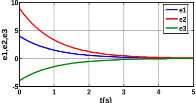
Thus, the error dynamics converges to the origin the state trajectories achieves anti-synchrony in finite time. The simulated results are depicted in Fig. 3 (a)-Fig. 3(c) and Fig. 4 respectively.
B. Case 2: Antisynchronization of Identical Burke-Shaw Systems
In this case, (2) is used as the identical equations for the drive and response systems respectively. Applying the nomenclature in case I, we can rewrite (2) in the following forms
'
'
'
d d
bs bs bs bs bs
d d d
bs bs bs bs bs
d d
bs bs bs bs bs
x x y
y y x z
z x y
(20)The response system becomes
'
'
'
r r
bs bs bs bs bs
r r r
bs bs bs bs bs
r r
bs bs bs bs bs
x x y
y y x z
z x y
(21)The error dynamics becomes
' 1
1 1 2
' 2 2 2 ' 3 3 ( ) ( )
( ) 2
bs r r d r bs bs bs bs bs r r d r
bs bs bs bs bs bs
e e e H
e e x z x z H
e x y x y H
(22)
The nonlinear control functions are defined as
1 1
2 2
3 3
( )
( ) ( )
( ) 2 ( )
bs
r r d r bs bs bs bs bs bs
r r d r bs bs bs bs bs bs
H L t
H x z x z L t
H x y x y L t
(23)
This reduces to a linear system with control inputs represented in the form
1 1 2 2 3 3 L e
L S e
S is a 3×3 matrice whose eigenvalues must lie in the negative real part such that (22) is asymptotically stable in finite time and is given by
1
2
3 0
0 1 0
0 0 ym ym (25) With
1 0; 2 0; 3 0
, the close loop system (22) is asymptotically stable. By inserting (25) in (24), (22) becomes
'
1 1 1
'
2 2 2
'
3 3 3
e e e e e e
(26)Theorem 2: The identical Burke-Shaw systems will anti-synchronized for any initial conditions
, ,
r d r d r d
x x y y z z provided the error dynamics converges asymptotically at the origin as t .
Proof: Adopt a Lyapunov function candidate,
2 2 2
1 2 3
1
( ) ( )
2 bs
V e e e e
(27)
' ' ' '
1 1 2 2 1 3
1
( ) ( )
bs
V e e e e e e e
(28)
By inserting (16) in (18),
' 1 2 2 2 3 2
1 2 3
( ) 0; i 0
bs bs bs
V e
e
e
e
(29)
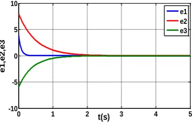
Thus, the error dynamics converges to the origin and the trajectories of the coupled systems achieves anti-synchrony in finite time. The simulated results are depicted in Fig. 5 and Fig. 6 respectively.
C. Case 3: Anti-Synchronization of Non-Identical Yu-Wang and Burke-Shaw Systems
Using (6) and (21), the drive and response systems are given as ' ' ' ' ( ) ( ) d d
ym ym ym ym
d d d
ym ym ym ym ym ym
d
ym ym ym
x y x
y x x z
z f t z
(30) ' ' ' r rbs bs bs bs bs
r r r
bs bs bs bs bs r r bs bs bs bs bs
x x y
y y x z
z x y
(31)
By adding (30) to (31), the error dynamics becomes
' 1
1
' 2
2
' ' 3
3
( )
( )
r r d d
bs bs bs bs ym ym ym as
r r r d d d
bs bs bs bs ym ym ym ym ym as
r r d
bs bs bs bs ym ym as
e x y y x U
e y x z x x z U
e x y f t z U
(32)
For the following values ym 10, ym 30, ym 2,
, 10
ym bs
; bs 4.272, (32) transforms to
' 1 1 1 ' 2 2 2 ' 3 3 3 10( )
10 30 2
2.5 10 4.272 sinh( )
2.5
r d
bs ym as
r r r d d d
ym bs bs ym ym ym as
r r d d
bs bs ym ym
r
bs as
e e y y U
e e y x z x x z U
e e x y x y
z U (33)
The nonlinear control functions are defined as
1 1
2 2
3
3
10( ) ( )
10 30 2 ( )
10 4.272 sinh( )
2.5 ( )
r d
as bs ym
r r r d d d
as ym bs bs ym ym ym
r r d d
as bs bs ym ym
r bs
U y y x t
U y x z x x z x t
U x y x y
z x t
(34) where 1 1 2 2 3 3 x e
x W e
x e
(35)1 0 0
0 1 0
0 0 2.5
W
(36)The eigenvalues of the matrice (36) are chosen such that it is Hurwitz. This leads to the following resolutions
1
2
3
1 0 0
0 1 0
0 0 2.5
W
(37)1 0; 2 0, 3 0
By inserting (37) in (35) and (34), the error dynamics (33) reduces to
'
1 1 1
'
2 2 2
'
3 3 3
e e e e e e (38)
Theorem 3: The Yu-Wang and Burke-Shaw systems will anti-synchronized for any initial conditions
, ,
r d r d r d
x x y y z z provided that the state trajectories of the error dynamics converges asymptotically at the origin as t .
Proof: Adopt a Lyapunov function candidate,
2 2 2
1 2 3
( ) ( )
2 bs
V e e e e
(39)
' ' ' '
1 1 2 2 1 3
( ) ( )
bs
V e e e e e e e
(40)
By inserting (16) in (18),
' 2 2 2
1 1 2 2 3 3
( ) 0; , i 0
Thus, the error dynamics converges to the origin and the trajectories of the coupled systems achieves anti-synchrony in finite time. The resulting plots are depicted in Fig. 7 and Fig. 8 respectively.
0 0.5 1 1.5 2 2.5 3
-4 -2 0 2 4
t(s)
x
d
,x
r
xd xr
(a)
0 0.5 1 1.5 2 2.5 3
-5 0 5 10
t(s)
y
d
,y
r
yd yr
(b)
0 0.5 1 1.5 2 2.5 3
-60 -40 -20 0 20 40
t(s)
zd
,zr
zd zr
(c)
Figure 3. Dynamics of the antisynchronized chaotic systems
0 0.5 1 1.5 2 2.5 3
-5 0 5 10
t(s)
e
1
,e
2
,e
3
e1 e2 e3
Figure 4. Asymptotic convergence of the error state vectors
V. SIMULATION RESULTS
A. Case 1: Identical Yu-Wang Systems
The identical Yu-Wang systems were simulated with MATLAB software for the following initial conditions:
Drive system, d( 0),d ( 0),d( 0) [3, 2, 10] ym ym ym
x y z
p and the
Response system, r( 0), r( 0),r( 0) [1, 6, 5] ym ym ym
x y z
q and error
system e1(0)4,e2(0)8,e3(0) 5 . The resulting
plots are depicted in Fig. 3 (a)-Fig. 3(c) and Fig. 4.
B. Case 2: Identical Burke-Shaw Systems
The identical Burke-Shaw systems were simulated with MATLAB software for the following initial
conditions: Drive system,
( 0), ( 0), ( 0) [1, 3, 10]
d d d
ym ym ym
x y z
p
and the Response system,
( 0), ( 0), ( 0) [3, 6, 6]
r r r
ym ym ym
x y z
q and
error system e1(0)4,e2(0)9,e3(0) 4 . The
resulting plots are depicted in Fig. 5 and Fig. 6.
0 1 2 3 4 5
-4 -2 0 2 4 6
t(s)
x
r,
x
d
xr xd
(a)
0 1 2 3 4 5
-10 -5 0 5 10 15
t(s)
y
r,
y
d
yr yd
(b)
0 1 2 3 4 5
-15 -10 -5 0 5 10
t(s)
zr
,zd
zr zd
(c)
Figure 5. Dynamics of the antisynchonized chaotic systems
0 1 2 3 4 5
-5 0 5 10
t(s)
e
1
,e
2
,e
3
e1 e2 e3
C. Case 3: Non-Identical Yu-Wang and Burke-Shaw Systems
The two non-identical systems were simulated for the same initial conditions as in case 1. The plotted are given in Fig. 7 and Fig. 8.
0 1 2 3 4 5
-3 -2 -1 0 1 2 3
t(s)
x
r,
x
d
xr xd
(a)
0 1 2 3 4 5
-4 -2 0 2 4 6 8
t(s)
y
r,
y
d
yr yd
(b)
0 1 2 3 4 5
-40 -20 0 20 40
t(s)
zr
,zd
zr zd
(c)
Figure 7. Dynamics of the antisynchronized chaotic systems
0 1 2 3 4 5
-10 -5 0 5 10
t(s)
e
1
,e
2
,e
3
e1 e2 e3
Figure 8. Asymptotic convergence of the error state vectors
VI. CONCLUSION
The Yu-Wang and Burke-Shaw systems synchronized in anti-phase via nonlinear active control strategy. The
positive constants and nonlinear hyperbolic functions of the system structures increases spectral densities to the systems and this can increase the complexity of the chaotic encryption keys when utilized in chaos-based secure communication scheme. The robustness of this simple antisynchronization scheme can be evaluated through observation of the antisynchronized dynamics in each case under study.
REFERENCES
[1] A. M. Harb and N. Abed-Jabar, “Controlling hopf bifurcation and chaos in a small power system,” Chaos, Solitons and Fractals, vol. 18, pp. 1055-1063, 2003.
[2] A. Kumar and B. M. Hegde, “Chaos theory: Impact on and applications in medicine,” Nitte Univ. J. Health Sci., vol. 2, no. 4, pp. 93-99, 2012.
[3] G. M. Maggio, O. D. Feo, and M. P. Kennedy, “Nonlinear analysis of the Colpitt oscillator and application to design,” IEEE Trans. Circ. Syst.-I: Fundamental Theory and Applications, vol. 46, no. 9, pp. 1118-1130, 1999.
[4] G. M. Hall, E. J. Holder, S. D. Cohen, and D. J. Gauthier, “Low-Cost chaotic radar design,” Proceedings of SPIE, vol. 8361, pp. 858-862, 2012.
[5] A. Al-Khedhairi, “The nonlinear control of food chain model using nonlinear feedback,” Applied Mathematical Sciences, vol. 13, no. 12, pp. 591-604, 2009.
[6] D. Guegan, “Chaos in economics and finance,” Annual Reviews in Control, vol. 33, no. 1, pp. 89-93, 2009.
[7] L. M. Pecora and T. L. Caroll, “Synchronization in chaotic systems,” Phys. Rev. Lett., vol. 64, pp. 821-824, 1990.
[8] E. Bollt, Y-C. Lai, and C. Grebogi, “Coding, channel capacity and noise resistance in communicating with chaos,” Phy. Rev. Letts., vol. 79, no. 19, pp. 3787-3790, 1997.
[9] B. Jovic, Synchronization Techniques for Chaotic Communication Systems, Springer-Verlag Berlin Heidelberg, 2011.
[10] K. M. Cuomo, A. V. Oppenheim, and H. S. Strogatz, “Synchronization of Lorenz-based chaotic circuits and application to secure communication,” IEEE Transaction on Circuits and Systems-II: Analogue and Digital Processing, vol. 40, no. 10, pp 626-633, 1993.
[11] S. S. Pawan, “Matlab simulation of chaotic systems and its application in secure communication with AWGN channel,” Int. J. Elect. Elect. Data Comm., vol. 1, no. 4, pp. 56-59, 2013.
[12] H. R. Abbasi, A. Gholami, M. Rostami, and A. Abbasi, “Investigation and control of unstable chaotic behaviour using chaos theory in electrical power systems,” Iranian Journal of Elect. Elect. Engg, vol. 7, no. 1, pp. 42-51, 2011.
[13] E. M. Shaverdiev, L. H. Hashimova, and N. T. Hashomova, “Chaos synchronization in some power systems,” Chaos, Solitons and Fractals, vol. 37, pp. 827-834, 3008.
[14] A. Khan, “Chaos synchronization and linear feedback control,” Int. Maths. Forum, vol. 5, no. 11, pp. 511-525, 2010.
[15] E. A. Umoh, “Chaos antisynchronization of the complex Deng’s toroidal system via hybrid feedback control,” Journal of Computational Intelligence and Electronics Systems,vol. 3, no. 2, pp. 138-142,2014.
[16] A. A. Emadzadeh and M. Haeri, “Antisynchronization of two different chaotic systems via active control,” WAST, vol. 6, pp. 62-65, 2005.
[17] D. Chen, W. Zhao, J. C. Sprott, and X. Ma, “Application of Takagi-Sugeno fuzzy models to a class of chaotic synchronization and antisynchronization,” Nonlinear Dynamics, vol. 73, no. 3, pp. 1495-1505, 2013.
[18] S. Hmmami and B. Mohammed, “Coexistence of synchronization and antisynchronization for chaotic systems via feedback control,” in Chaotic Systems, E. Tielo-Cuautle, Ed., InTech, 2011. [19] S. Vaidyanathan, “Global chaos synchronization of hyperchaotic
Newton-Lepnik system by sliding mode control,” Int. J. Info. Tech. Conv. Serv., vol. 1, no. 1, pp. 34-43, 2011.
[21] R. Shaw, “Strange attractors, chaotic behaviour and information flow,” Zeitschrift Fur Naturforsch A, vol. 36, pp. 80-112, 1981. [22] C. Letellier, T. Tsankov, G. Bryne, and R. Gilmore, “Large-Scale
structural reorganization of strange attractor,” Physical Review E, vol. 72, no. 2, pp. 986-1023, 2005.