www.geosci-model-dev.net/9/1673/2016/ doi:10.5194/gmd-9-1673-2016
© Author(s) 2016. CC Attribution 3.0 License.
ICESHEET 1.0: a program to produce paleo-ice sheet
reconstructions with minimal assumptions
Evan J. Gowan1,2,3, Paul Tregoning3, Anthony Purcell3, James Lea4,1,2, Oscar J. Fransner5, Riko Noormets5, and J. A. Dowdeswell6
1Department of Physical Geography, Stockholm University, Stockholm, Sweden 2Bolin Center for Climate Research, Stockholm, Sweden
3Research School of Earth Science, The Australian National University, Canberra, Australia 4School of Environmental Sciences, University of Liverpool, Liverpool, UK
5Department of Arctic Geology, The University Center in Svalbard (UNIS), Longyearbyen, Norway 6Scott Polar Research Institute, Cambridge, UK
Correspondence to: Evan J. Gowan ([email protected])
Received: 13 January 2016 – Published in Geosci. Model Dev. Discuss.: 20 January 2016 Revised: 22 April 2016 – Accepted: 22 April 2016 – Published: 3 May 2016
Abstract. We describe a program that produces paleo-ice sheet reconstructions using an assumption of steady-state, perfectly plastic ice flow behaviour. It incorporates three in-put parameters: ice margin, basal shear stress and basal to-pography. Though it is unlikely that paleo-ice sheets were ever in complete steady-state conditions, this method can produce an ice sheet without relying on complicated and unconstrained parameters such as climate and ice dynam-ics. This makes it advantageous to use in glacial-isostatic adjustment ice sheet modelling, which are often used as in-put parameters in global climate modelling simulations. We test this program by applying it to the modern Greenland Ice Sheet and Last Glacial Maximum Barents Sea Ice Sheet and demonstrate the optimal parameters that balance computa-tional time and accuracy.
1 Introduction
Reconstructing past ice sheets is a complex task, due to the large number of parameters that can affect their growth and retreat. For example, Tarasov et al. (2012) presented a glacial systems model that contained 39 parameters that could be tuned, which included climatology, Earth rheology, ice physics and margin chronology. Many of these parame-ters are poorly constrained by available observations. In par-ticular, past climate is often parameterized based on ice core
data from Greenland and Antarctica, or reconstructions from speleothems that are located far from where the ice sheets existed.
Since past climatic parameters are generally only well characterized in areas outside of where paleo-ice sheets ex-isted, ice sheet reconstructions that are independently deter-mined using evidence of glacial-isostatic adjustment (GIA) are often used in paleo-climate simulations (e.g. Braconnot et al., 2007, 2012). One of the most commonly used GIA based reconstructions of glaciation is the ICE-xG series (e.g. Peltier, 2004; Peltier et al., 2015). They produce configura-tions of ice sheets that minimize the misfits of geodetic and relative sea level data, with limited regard to the physical realism of the ice sheet itself. Another commonly used re-construction is the ANU model (e.g. Lambeck et al., 2010), which was developed using an assumed peak ice elevation at the centre of ice sheets, and using a parabolic ice profile to the margins. In their formulation, each flowline ray is al-lowed to have different basal shear stress values, but is less flexible in regards to the direction of the flowline, and spatial variability in basal shear stress along it.
re-constructions that have limited or no physics applied to their construction, and the full glacial systems models that demand considerable computational resources. The reconstructions are based on the assumption of perfectly plastic, steady-state ice conditions. It allows for the rapid determination of paleo-ice sheet configurations, which is desirable when matching observations of GIA. We present an example application of this program to the Barents Sea Ice Sheet, a relatively short-lived portion of the Eurasian Ice Sheet complex, by trying to match an existing GIA based model. We also apply the model to the contemporary Greenland ice sheet to provide an indication of how well the model is capable of reconstructing a known ice sheet geometry. Ultimately, the goal would be to reconstruct, in a timestepped fashion, the entire history of an ice sheet complex. In this case, the basal topography is rel-atively well determined (since there is no existing ice), and the basal shear stress can be established to a certain extent by the surficial geology and geomorphology. The ice topogra-phy and basal shear stress are determined through time using external evidence, such as the nature of GIA. An example of this is presented for the western Laurentide Ice Sheet by Gowan et al. (2016).
2 Methodology 2.1 Theory
The reconstructions produced by the ICESHEET program are based on the assumption that ice rheology adheres to perfectly plastic, steady-state conditions (i.e. ignoring lateral shear stresses, and assuming that the ice surface is not dy-namically changing). The two-dimensional form of this the-ory was derived by Nye (1952), and neglects variability in topography and longitudinal changes in stress. In this equa-tion, the ice surface gradient is directly related to the strength of the ice–bed interface, or basal shear stress. The basal shear stress is related to a number of factors, including basal geol-ogy, sediment thickness and strength, hydrolgeol-ogy, temperature and bed roughness.
dE
ds = τo ρigH
(1)
The ice surface elevation is E,s is the distance along ice flowline profile, τo is the shear stress at the base of the ice
sheet, which balances the driving stress,ρi is the density of
ice,g is the gravity at the Earth’s surface, andH is the ice thickness. If the distance from the ice sheet margin to the centre of the ice sheet is known, then the thickness along the profile between the two points can be calculated using the following formula (Cuffey and Paterson, 2010).
H2=2τo
ρig
[L−x] (2)
In this equation,Lis the distance between the margin and centre of the ice sheet, andx is the distance from the cen-tre. Though this equation is simple, it can be used to make a rough estimate of the thickness of ice sheets, neglecting basal topography (Cuffey and Paterson, 2010). Equation (2) was used to create the ANU ice sheet reconstructions (i.e. Lambeck et al., 1998, 2006, 2010). The weakness of using this equation is that the centre of the ice sheet has to be as-sumed a priori. It also does not take into account changing basal shear stress conditions or changes in topography.
In order to overcome problems with spatial changes in basal topography and shear stress, in addition to the uncer-tainties in the location of the ice sheet centre, Reeh (1982) and Fisher et al. (1985) presented expanded version of Eq. (1) that allows for changes in the direction of the flowline. The equation becomes the following partial differential equation.
d
E
ds
2
=
∂E ∂x
2
+
∂E ∂y
2
(3) The coordinate system is set up so thatx points towards the centre of the ice sheet, andy is parallel to the margin. Pre-sented in the notation used by Reeh (1982), Eq. (1) is sub-stituted into the left side of Eq. (3) with the ice thickness represented in terms of ice surface elevation and basal topog-raphy elevationB, and substituting in a characteristic thick-ness,Hf =τo/ρig.
H
f E−B
2
=
∂E
∂x
2
+
∂E
∂y
2
(4) The above equation describes the change in ice thickness over an arbitrary surface. This partial differential equation can be solved by the method of characteristics (Kamke, 1965). Thex andy partial derivatives in Eq. (4) are sub-stituted byp=∂E/∂x andq=∂E/∂y, then rearranged in terms ofp.
p=
s H
f E−B
2
−q2 (5)
The solution to the partial differential equation then becomes three ordinary differential equations that are solved simulta-neously, using the method of characteristics (Reeh, 1982). dy
dx = q
p (6)
dE
dx =
p2+q2
p =
Hf2
dq
dx =
(p2+q2)(∂B/∂y−q) p(E−B)
= H
2
f
p(E−B)3
∂B ∂y −q
(8) Equation (6) gives the direction of local maximum steep-ness, while the other two equations describe how the eleva-tion changes spatially in thex direction. Fisher et al. (1985) expanded Eq. (8) to allow for changes in basal shear stress (in terms of the characteristic thickness,Hf).
dq
dx = Hf2
p(E−B)3
∂B
∂y −q
+
H
f
p(E−B)2
∂H
f
∂y (9)
These equations are solved by numerical integration to deter-mine the course and gradient of an ice flowline. In the next subsection, we note some of the improvements to the original methodology, including adjustments to the base topography with realistic GIA, dealing with margins that are in marine environments, automatic determination of ice sheet saddles, and adjusting for the presence of nunataks.
It is important to note that assuming perfectly plastic, steady-state conditions for the ice sheet is not accurate in ar-eas where the ice sheet was highly dynamic, or where lateral shear stress was an important factor. Due to this, the output basal shear stress is unlikely to reflect the true basal shear stress in those areas.
2.2 Algorithm to reconstruct ice sheets
In order to solve Eqs. (6)–(8), initial values for E,y andq
are required. Starting the calculation at the margin is conve-nient from the perspective of reducing a priori assumptions on ice distribution, though it leads to a singularity because the ice thickness is zero (E=B). Consequently, the value of
E at the margin must be set to be a nominal value (in the sample problems presented in this study, 1 m). Although the actual thickness of ice near the margin may be as high as tens of metres, the choice of starting value will not have a large effect on the final model. For instance, the distance from the margin required in Eq. (2) to reach 10 m from a starting value of 1 m, and a low basal shear stress value (5 kPa) is 90 m, substantially smaller than the uncertainty in the margin lo-cation for paleo-ice sheets (Clark et al., 2012; Gowan, 2013; Hughes et al., 2016). For simplicity, the value ofqis defined to be zero at the margin. This can be justified because near the margin the value of termHf/(E−B)will dominate Eq. (5)
in the defined coordinate system.
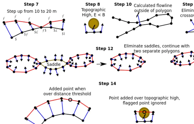
The ice sheet reconstruction is calculated in a piece-wise manner (see Fig. 1 for an illustration of the steps involved). The ice flowline calculation is initiated at intervals along the margin, which are user defined. The flowline calculation pro-ceeds until it reaches a particular elevation (a user defined
contour interval), at which point the program checks to see if any flowlines cross over, or if a saddle point in the ice sheet has been reached. A sequential list of the modelling steps is given below.
1. All parameters (ice sheet margin, shear stress map, to-pography map) are converted from geographical coor-dinates to a Cartesian coordinate system prior to the ex-ecution of the program.
2. Estimates of the basal shear stress for the area of interest are read into the program. The shear stress values must be adjusted for each time epoch to produce an appropri-ate ice sheet configuration.
3. The basal topography data for the area of interest are read in. For the first iteration of ice sheet model de-velopment, it uses modern topography or topography adjusted for changes in global mean sea level (in prac-tice, it has limited impact on the final reconstruction, i.e.
<100 m near the edge of the ice sheet and much less than that in the interior, even with predominantly ma-rine based ice sheets). In subsequent iterations, the to-pography is adjusted for glacial-isostatic adjustment, to take into account the fact that the ice sheet will deform the Earth, and that the ice sheets will cause changes to sea level. The modified topography is calculated before running the ice sheet program. In the Barents Sea Ice Sheet sample problem, we use the CALSEA program to calculate GIA (Nakada and Lambeck, 1987; Lam-beck et al., 2003). CALSEA computes glacial-isostatic adjustment using a spherically symmetric Earth, with a Maxwell rheology mantle and elastic lithosphere, using the PREM model (Dziewonski and Anderson, 1981) for other Earth model parameters. In includes time evolving shorelines and rotational feedback.
4. The program reads in the margin, and defines locations along the perimeter where the flowline calculation initi-ates. The minimum distance along the margin between where flowline calculation is initiated is user-defined. The program defines the initial direction of flow to be perpendicular to the margin, away from the centre of the ice sheet.
5. The margin is set to have an initial ice thickness of 1 m. If the margin is located where the topography is be-low sea level, it is assumed that the margin corresponds to the grounding line of the ice sheet. A conservative estimate of the thickness of ice at this point is set to
x
Step 8 TopographicHigh, E < B
x
Step 10 Calculated flowline outside of polygon
10 12 16
21 17 15
20 20 20 20 20
Step 7 Step up from 10 to 20 m
x
Step 11 Eliminate crossoversStep 12
Saddle
Eliminate saddles, continue with two separate polygons
Step 14 Added point when
over distance threshold
x
Point added over topographic high, flagged point ignored
Figure 1. Schematic illustrating the steps in calculating the ice sheet, illustrating steps 7, 8, 10, 11, 12 and 14 in Sect. 2.2. The black lines
indicate the initial elevation contour, blue lines indicate calculated flowlines, red lines indicate the next elevation contour, black circles indicate flowline initiation points, unfilled circles indicate added initiation points for the next elevation contour, crosses indicate flagged points that are not included in the next elevation contour.
basal shear stress values. If it is, the ice thickness at the point with the lower elevation is increased. This check is only done whereB <0.
6. The calculation of ice elevation contours is a recursive process. If the contour crosses over itself (signifying a saddle on the surface of the ice sheet), the contour poly-gon is split, and the calculation is continued as separate polygons (see step 12).
7. The program searches for points on the contour that are below the next contour elevation. The elevation may be above the next contour elevation along the margin, or if a point coincides with a nunatuk (see step 14). It then calculates the flowline by numerical integration of Eqs. (6)–(8), using the Runge–Kutta method (Press, 1992). When it reaches the next contour elevation, the calculation stops.
8. If the flowline calculation cannot reach the next contour elevation, which happens when the topography is too high (H→0, orE < B), the point is flagged and not included in the next contour (Fig. 1).
9. If the flowline direction changes sufficiently so that
q≥Hf/(E−B)(i.e.papproaches zero), the local
co-ordinate system is rotated so thatpis in the direction of maximum flow.
10. If the calculated flowline goes outside the last calculated contour polygon, it is flagged and the point is not in-cluded in the next contour. This happens when the ice surface is near its peak height. This can also happen in
areas where there is a sudden change in topography or basal shear stress, which causes a deflection in the flow-line direction (Fig. 1).
11. After the flowlines are calculated for each applicable point along the polygon, the program checks to see if any of the calculated flowlines cross over. Offending crossovers are eliminated using a motorcycle algorithm (e.g. Vigneron and Yan, 2014). The eliminated flowlines are flagged and not included in the next contour (Fig. 1). 12. At this point, an initial polygon of the next elevation contour can be constructed. This is checked to ensure that it is a simple polygon (i.e. a polygon that does not cross over itself). If it is not, then the program breaks it into several polygons, and determines whether they represent domes (ice gradient is increasing towards the centre of the polygon) or saddles (the ice gradient is de-creasing towards the centre of the polygon). Where a saddle is identified, it is determined to have reached its peak elevation and is eliminated from subsequent calcu-lations (Fig. 1).
13. The ice elevation and thickness for all points on a valid polygon (including flagged points) are written to file. 14. The polygon is resampled using the user-defined
points, and may incorporate basal topographic highs, where flowline calculation will not be initiated (Fig. 1). This process is repeated for each time interval of interest. After calculation of the ice reconstruction, the calculated ele-vation values are averaged into a grid to be used as input for a GIA calculation program. The grid is created using a contin-uous smoothing algorithm, which is part of Generic Mapping Tools (Smith and Wessel, 1990).
3 Sample reconstruction – Barents Sea Ice Sheet 3.1 Setup
The Barents Sea Ice Sheet was predominantly marine based, and likely formed by the merging of isolated ice caps over Svalbard, Franz Josef Land, Novaya Zemlya and the Scan-dinavia Ice Sheet (Ingólfsson and Landvik, 2013). The hy-pothesis explaining the glaciation of the entire Barents Sea is that GIA warped the floor of the Barents Sea upwards, favouring the formation of grounded ice. At the Last Glacial Maximum (LGM) (about 20 ka), the ice sheet covered the entire continental shelf region west of Novaya Zemlya (In-gólfsson and Landvik, 2013). The extent was probably lim-ited in the Kara Sea east of Novaya Zemlya, compared to the mid-Weichselian (45–55 ka) glaciation. At the LGM, the ice thickness was likely greatest to the east of Svalbard, on the basis of the pattern of paleo-sea level reconstructions (Lam-beck, 1995).
In this sample problem, the ice sheet extent is taken as the “most likely” configuration at 20 ka from the DATED project (Hughes et al., 2016). Since the Barents Sea Ice Sheet merged with the Scandinavian Ice Sheet at the LGM, the margin is cut off far enough south so that the northern part of the Scan-dinavian Ice Sheet is sufficiently represented. The basal to-pography used in this problem is from IBCAO (Jakobsson et al., 2012). The basal topography of Svalbard takes into account the thickness of modern ice cover. There is no pub-lished information on the thickness of ice on Novaya Zemlya, so we use contemporary ice surface topography. The basal shear stress was initially parameterized on the basis of to-pography and bedrock geology. The values were adjusted in order to produce an ice thickness distribution that is similar to the GIA based ANU model (Lambeck, 1995; Lambeck et al., 2006, 2010). Exact matching of ice thickness in the sample problem to the ANU model was not attempted, since it is of low resolution, and has a different margin configuration to that of Hughes et al. (2016). Specifically, it is less extensive along the Bear Island Trough. In order to approximate the ice thickness from the ANU model, the basal shear stress was set to be high along the northern part of the ice sheet, and rela-tively low in the southern Barents Sea. Both the topography and basal shear stress values are sampled at 5 km (Fig. 2).
This purpose of this test is to demonstrate that GIA has an impact on the ice sheet reconstruction. This test only
in-0 500km
−1000 0 1000 2000 3000
Topography (m)
0 500km
0 20 40 60 80 100 120
Shear stress (kPa)
Kara Sea Sv
Sv
FJL FJL BRT
BRT
NZ NZ Scandinavia
Scandinavia
(a) (b)
Figure 2. Basal topography used in the resolution test, which is
modern topography minus the 133 m drop in global mean sea level at 20 ka. Also shown in brown is the 20 ka ice margin (Hughes et al., 2016) and the location of places described in the text. Sv – Svalbard. FJL – Franz Josef Land. NZ – Novaya Zemlya. BRT – Bear Island Trough. (b) Basal shear stress values used in the example in this paper.
cludes the Barents Sea Ice Sheet for the calculation of GIA. In a full glacial reconstruction (e.g. Gowan et al., 2016), it is necessary to include the effects of far field ice sheets, and realistic ice sheet growth and decay.
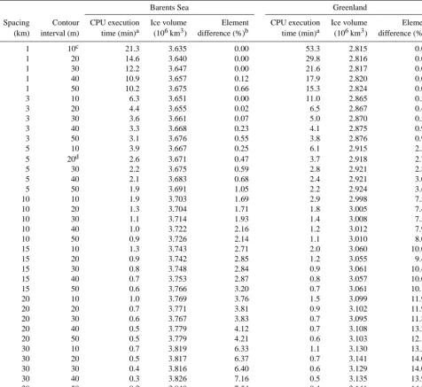
3.2 Resolution test
In order to test the optimal parameters for producing ice sheet reconstructions, a series of tests with different distance and contour intervals were performed, the results can be found in Table 1. This test involved using modern topography minus the approximate 133 m reduction in global mean sea level at 20 ka (Fig. 2, Lambeck et al., 2014). The shear stress and basal topography values are shown in Fig. 2. Figure 3 shows how changes in basal shear stress and basal topography af-fect the modelled ice sheet. The spacing between contours is greater in areas of low basal topography and shear stress, which replicates ice flow from areas of high to low basal to-pography, and around barriers that resist ice flow.
Table 1. Results of the resolution test
Barents Sea Greenland
Spacing Contour CPU execution Ice volume Element CPU execution Ice volume Element (km) interval (m) time (min)a (106km3) difference (%)b time (min)a (106km3) difference (%)b
1 10c 21.3 3.635 0.00 53.3 2.815 0.00
1 20 14.6 3.640 0.00 29.8 2.816 0.00
1 30 12.2 3.647 0.00 21.6 2.817 0.00
1 40 10.9 3.657 0.12 17.9 2.820 0.01
1 50 10.2 3.675 0.66 15.3 2.824 0.05
3 10 6.3 3.651 0.00 11.0 2.865 0.33
3 20 4.4 3.655 0.02 6.5 2.867 0.46
3 30 3.6 3.661 0.07 5.0 2.870 0.53
3 40 3.3 3.668 0.23 4.1 2.875 0.94
3 50 3.1 3.676 0.55 3.8 2.876 0.98
5 10 3.9 3.667 0.25 6.1 2.915 2.53
5 20d 2.6 3.671 0.47 3.7 2.918 2.79
5 30 2.2 3.675 0.59 2.8 2.921 2.89
5 40 2.1 3.683 0.68 2.4 2.921 3.05
5 50 1.9 3.691 1.05 2.2 2.924 3.68
10 10 1.9 3.703 1.69 2.9 2.998 7.53
10 20 1.3 3.704 1.71 1.8 3.005 7.47
10 30 1.1 3.714 1.93 1.4 3.008 7.51
10 40 1.0 3.722 2.16 1.2 3.012 7.94
10 50 0.9 3.726 2.14 1.1 3.010 8.02
15 10 1.3 3.743 2.71 2.0 3.060 10.07
15 20 0.9 3.742 2.85 1.2 3.055 9.44
15 30 0.8 3.748 2.84 0.9 3.061 10.45
15 40 0.7 3.753 2.87 0.8 3.057 10.04
15 50 0.6 3.766 3.20 0.7 3.061 10.18
20 10 1.0 3.769 3.76 1.5 3.099 11.99
20 20 0.7 3.771 3.81 0.9 3.102 11.95
20 30 0.6 3.767 3.83 0.7 3.095 11.84
20 40 0.5 3.779 4.12 0.7 3.108 13.29
20 50 0.5 3.779 4.21 0.6 3.103 12.19
30 10 0.7 3.819 6.33 1.1 3.130 13.55
30 20 0.5 3.817 6.37 0.7 3.141 14.04
30 30 0.4 3.816 6.40 0.6 3.129 14.01
30 40 0.3 3.826 7.16 0.5 3.135 13.92
30 50 0.3 3.840 7.54 0.4 3.141 14.24
aExecution time on Terrawulf III (Sambridge et al., 2009), Dual Intel Xeon X5650 at 2.66 GHz running OpenSuse 13.2. Compiled with ifort 15 with -O2 flag.bPercent of
0.5◦longitude by 0.25◦elements that are>100 m different from the reference model (out of 23 205 total elements for the Barents Sea, and 21 901 for Greenland).
cReference reconstructions.dRecommended reconstructions.
Scandinavia. There is a tendency towards overestimating the ice thickness when the initiation distance is larger than 5 km (Fig. 4). During the initial phases of GIA based ice model de-velopment, it may be prudent to decrease the resolution of the grids to quickly determine an estimate of basal shear stress, then increase the resolution when refinement is necessary.
3.3 GIA test
When an ice sheet grows, the basal topography is modi-fied by GIA, which will significantly impact the Barents Sea Ice Sheet example. Therefore, in order to obtain an
100 200 300 300 400 500 500 700 700 700 800 800 900 900 1000 1000 1000 1100 1100 1100 1200 1200 1200 1300 1300 1300 1400 1400 1400 1400 1500 1500 1500 1500 1600 1600
0 20 40
km
−1000 0 1000 2000
Topography (m) 100 300 300 400 500 500 700 700 700 800 800 900 900 1000 1000 1000 1100 1100 1100 1200 1200 1200 1300 1300 1300 1400 1400 1400 1400 1500 1500 1500 1500 1600
0 20 40
km
0 20 40 60 80 100 120
Shear stress (kPa) 16001600
Figure 3. Example from central–western Svalbard of how spatial
changes in basal topography and basal shear stress affect the re-constructed ice surface topography of the ice sheet (see text). The contour interval is 100 m in the figure, though this sample was cal-culated with a 5 km spacing and 20 m contour interval. The dark black lines are the modern-day coastlines.
levels at 10 ka. After the first iteration of GIA, the ice sheet contribution to global mean sea level is subtracted to deter-mine the Earth deformation. When combined with the actual global mean sea level at this time (−133 m), it should give a reasonable estimate of local basal topography.
The results show that one iteration of GIA has a significant effect on ice sheet reconstruction, and in this case increases the total volume by about 5.8 % (Fig. 5). In addition, since the basal topography becomes more depressed towards the centre of the ice sheet relative to the initial reconstruction, the reconstructed ice surface topography is lower and has a more gentle gradient. A second iteration of GIA had only a minor effect on the reconstructed ice sheet (0.4 % increase in volume from the first iteration).
Additional tests by Gowan (2014) for the full deglacial Laurentide Ice Sheet showed that there is only a weak depen-dence on reconstructed ice volume and the Earth model used to compute GIA. For three layer (lithosphere, upper man-tle, lower mantle) Earth models, the ice volume varied most with changes in lower mantle viscosity at LGM extent, but the difference was less than 0.5 % (though smaller ice sheets will have less dependence on the lower mantle). Towards the end of deglaciation, there was more dependence on upper mantle viscosity, but again, the volume difference was less than 0.5 %. Though the volume was close to the same, there were slight differences in the distribution of ice, though not by more than 100 m in extreme cases. Therefore, the recom-mendation when creating an ice sheet model is to include at least one iteration of GIA, but the chosen Earth model is not as important. 0 0 0 25 250 250 0 250 500 500 0 500 750 750 750 750 1000 1000 1000 1000 1250 1250 1250 1250 1500 1500 1500 1750 1750 2000 2000 2250 2250
0 500km
0 1000 2000 3000
Ice surface elevation (m)
100 100
100
0 500km
−500 −250 0 250 500
Ice surface difference (m)
(a) (b)
Figure 4. (a) Reference ice sheet reconstruction with a 1 km
spac-ing and 10 m contour interval usspac-ing the topography and basal shear stress in Fig. 2. (b) The difference between a model calculated with a 20 km spacing and 20 m contour interval and the reference recon-struction shown in (a). This demonstrates that the lower resolution tends to overestimate the ice surface elevation in mountainous re-gions. −100 −100 −50 −50 −50 0 0 0 0
0 500km
−200 −100 0 100 200
Ice surface difference (m)
50 50 50 100 100 100 150
0 500km
−200 −100 0 100 200
Ice thickness difference (m) 0 0 0 25 250 250 0 250 500 500 500 750 750 750 750 1000 1000 1000 1000 1250 1250 1250 1500 1500 1500 1750 1750 2000 2000
0 500km
0 1000 2000 3000
Ice surface elevation (m)
0 0 0 250 250 250 500 500 500 750 750 750 750 1000 1000 1000 1000 1250 1250 1250 1500 1500 1500 1750 1750 1750 2000 2000 22502500
0 500km
0 1000 2000 3000
Ice thickness (m)
(a) (b)
(c) (d)
Figure 5. Ice sheet reconstruction after one iteration of GIA. (a) Ice
surface elevation. (b) Ice thickness. (c) Difference in elevation be-tween (a) and the initial model without GIA deformed topography.
(d) Same as (c) but for ice thickness.
4 Sample reconstruction – Greenland Ice Sheet 4.1 Setup
continuity based inversion of the contemporary ice thick-ness (Morlighem et al., 2014). Reeh (1982) reconstructed the Greenland Ice Sheet reasonably well using the method-ology explained earlier using a constant basal shear stress of 90 kPa. Since ICESHEET can have spatially variable basal shear stress and account for variable topography, it is possi-ble to refine this. Advances in remote sensing over the last 30 years also allow a more accurate comparison to contem-porary topography.
The goal of this example is to determine the misfit be-tween the ICESHEET reconstructed ice surface topography and the contemporary ice sheet using a methodology anal-ogous to the reconstruction of a paleo-ice sheet. The input grounded ice margin and basal topography data come from the IceBridge BedMachine Greenland, Version 2 data set (Morlighem et al., 2014, 2015). The basal shear stress value domains were designed the same way as a paleo-ice sheet would be constructed. The domains were constructed purely on the basis of basal topography (Fig. 6), since information on basal geology is limited. They were predominantly di-vided into areas of rugged topography (i.e. mountainous re-gions), flat-lying areas, and fjords. There intentionally was no attempt to divide it on the basis of modern ice flow pat-terns, given that it may not be possible to deduce them for a paleo-ice sheet. The shear stress values in the domains were adjusted iteratively in order to try to match the observed ice surface topography. In a paleo-ice sheet, it will not be possi-ble to know what the ice surface topography was a priori. In that case, other sources of data (i.e. GIA) must be used as the basis for the reconstruction.
4.2 Results
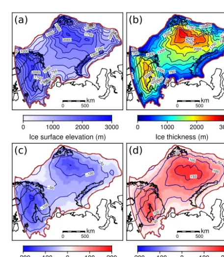
The resulting reconstruction is shown in Fig. 6. For compari-son purposes, the ice sheet is averaged into a 25 km grid. The reconstructed ice sheet surface topography has an average difference of−37±2 m (within 200 m of the true topogra-phy for most of the ice sheet). The largest errors (>400 m) occur in places where there are narrow ice streams near the edge of the ice sheet, which could not be parameterized us-ing the coarse resolution shear stress domains. In general, the shear stress values are highest in the mountainous regions in southeastern Greenland. The basal shear stress is lowest in the centre of the ice sheet, likely reflecting the flat-lying basal topography. Direct inversions for basal shear stress have only been performed for some of the ice streams in (e.g. Sergienko et al., 2014; Shapero et al., 2016). In the study by Sergienko et al. (2014), the basal shear stress exhibited a banded pat-tern, alternating between low (<50 kPa) to high (>150 kPa) values over spatial ranges of 5–20 km. Shapero et al. (2016) found that the basal shear stress directly under fast flowing ice streams was almost negligible, but at the sides it could exceed 375 kPa. If averaged over a larger area, these values are consistent with the 100–200 kPa values in our reconstruc-tion (Fig. 6).
Figure 6. Sample reconstruction of the contemporary Greenland
Ice Sheet. (a) Modern topography. The brown line is the current grounded ice margin, the black lines are the modern day coastlines.
(b) Reconstructed topography. (c) Final iterated basal shear stress
domains and values used for the reconstruction. (d) Difference be-tween the observed topography and reconstructed topography.
From Table 1, the reconstructed volume is within 5 % of this value, except in the lowest resolution tests.
5 Conclusions
ICESHEET 1.0 is a program that can quickly create recon-structions of paleo-ice sheets, with a given margin configura-tion and estimated basal shear stress. We have provided two proof of concept examples showing reconstructions of the modern Greenland Ice Sheet and the Barents Sea Ice Sheet at the LGM. It is recommended that at least one iteration of GIA is included to best characterize the thickness and ice surface topography. It is also recommended (if a 5 km basal topog-raphy grid is used) to use a flowline spacing interval of 5 km and contour interval of 20 m for optimal calculation speed. This program has been used to create a full late glacial GIA based ice sheet reconstruction of the western Laurentide ice sheet (Gowan et al., 2016). It is ideal for producing ice sheet reconstructions that have minimal input assumptions, but are glaciologically plausible. A suite of ice sheet reconstructions through a glacial cycle could be used as independent inputs for climate and ice sheet dynamics modelling.
Code availability
The source code, licensed under GPL version 3, and Green-land Ice Sheet example are available in the Supplement. Software updates will be available on EJG’s website (http: //www.raisedbeaches.net).
The Supplement related to this article is available online at doi:10.5194/gmd-9-1673-2016-supplement.
Acknowledgements. The ICESHEET program was developed
as part of a PHD project by EJG, and was funded by an ANU Postgraduate Research Scholarship. This study is funded as part of a Swedish Research Council FORMAS grant (grant 2013-1600) to Nina Kirchner. We thank Nina Kirchner for comments that improved this paper. Computing resources used for the develop-ment of ICESHEET were provided by Terrawulf (Sambridge et al., 2009). We thank Anna Hughes for providing the DATED margin at 20 ka prior to its publication. We also thank Kurt Lambeck for allowing us to use the ANU model as a template for the Barents Sea Ice Sheet example. Figures were created using GMT (Wessel and Smith, 1991).
Edited by: D. Goldberg
References
Braconnot, P., Otto-Bliesner, B., Harrison, S., Joussaume, S., Pe-terchmitt, J.-Y., Abe-Ouchi, A., Crucifix, M., Driesschaert, E.,
Fichefet, Th., Hewitt, C. D., Kageyama, M., Kitoh, A., Laîné, A., Loutre, M.-F., Marti, O., Merkel, U., Ramstein, G., Valdes, P., Weber, S. L., Yu, Y., and Zhao, Y.: Results of PMIP2 coupled simulations of the Mid-Holocene and Last Glacial Maximum – Part 1: experiments and large-scale features, Clim. Past, 3, 261– 277, doi:10.5194/cp-3-261-2007, 2007.
Braconnot, P., Harrison, S. P., Kageyama, M., Bartlein, P. J., Masson-Delmotte, V., Abe-Ouchi, A., Otto-Bliesner, B., and Zhao, Y.: Evaluation of climate models using palaeoclimatic data, Nature Climate Change, 2, 417–424, doi:10.1038/nclimate1456, 2012.
Clark, C. D., Hughes, A. L., Greenwood, S. L., Jordan, C., and Sejrup, H. P.: Pattern and timing of retreat of the last British-Irish Ice Sheet, Quaternary Sci. Rev., 44, 112–146, doi:10.1016/j.quascirev.2010.07.019, 2012.
Cuffey, K. M. and Paterson, W. S. B.: The physics of glaciers, Else-vier, Burlington, MA, USA, 2010.
Dziewonski, A. M. and Anderson, D. L.: Preliminary refer-ence Earth model, Phys. Earth Planet. In., 25, 297–356, doi:10.1016/0031-9201(81)90046-7, 1981.
Fisher, D., Reeh, N., and Langley, K.: Objective reconstructions of the Late Wisconsinan Laurentide Ice Sheet and the significance of deformable beds, Géogr. Phys. Quatern., 39, 229–238, 1985. Gowan, E. J.: An assessment of the minimum timing of ice free
conditions of the western Laurentide Ice Sheet, Quaternary Sci. Rev., 75, 100–113, doi:10.1016/j.quascirev.2013.06.001, 2013. Gowan, E. J.: Model of the western Laurentide Ice Sheet, North
America, PhD thesis, The Australian National University, Can-berra, ACT, Australia, 2014.
Gowan, E. J., Tregoning, P., Purcell, A., Montillet, J.-P., and Mc-Clusky, S.: A model of the western Laurentide Ice Sheet, us-ing observations of glacial isostatic adjustment, Quaternary Sci. Rev., 139, 1–16, doi:10.1016/j.quascirev.2016.03.003, 2016. Hughes, A. L., Gyllencreutz, R., Lohne, Ø. S., Mangerud, J., and
Svendsen, J. I.: The last Eurasian ice sheets – a chronological database and time-slice reconstruction, DATED-1, Boreas, 45, 1–45, doi:10.1111/bor.12142, 2016.
Ingólfsson, Ó. and Landvik, J. Y.: The Svalbard–Barents Sea ice-sheet–Historical, current and future perspectives, Quaternary Sci. Rev., 64, 33–60, doi:10.1016/j.quascirev.2012.11.034, 2013. Jakobsson, M., Mayer, L., Coakley, B., Dowdeswell, J. A., Forbes,
S., Fridman, B., Hodnesdal, H., Noormets, R., Pedersen, R., Rebesco, M., Schenke, H. W., Zarayskaya, Y., Accettella, D., Armstrong, A., Anderson, R. M., Bienhoff, P., Camerlenghi, A., Church, I., Edwards, M., Gardner, J. V., Hall, J. K., Hell, B., Hestvik, O., Kristoffersen, Y., Marcussen, C., Mohammad, R., Mosher, D., Nghiem, S. V., Pedrosa, M. T., Travaglini, P. G., and Weatherall, P.: The international bathymetric chart of the Arctic Ocean (IBCAO) version 3.0, Geophys. Res. Lett., 39, L12609, doi:10.1029/2012GL052219, 2012.
Kamke, E.: Differentialgleichungen lösungsmethoden und lösun-gen. Bd. II. Partielle Differentialgleichungen erster Ordnung fur eine gesuchte Funktion, Akademische Verlagsgesellschaft Geest und Portig K.G., Leipzig, 1965.
Eu-rope, Geophys. J. Int., 134, 102–144, doi:10.1046/j.1365-246x.1998.00541.x, 1998.
Lambeck, K., Purcell, A., Johnston, P., Nakada, M., and Yokoyama, Y.: Water-load definition in the glacio-hydro-isostatic sea-level equation, Quaternary Sc. Rev., 22, 309–318, doi:10.1016/S0277-3791(02)00142-7, 2003.
Lambeck, K., Purcell, A., Funder, S., Kjær, K. H., Larsen, E., and Moller, P.: Constraints on the Late Saalian to early Middle We-ichselian ice sheet of Eurasia from field data and rebound mod-elling, Boreas, 35, 539–575, doi:10.1080/03009480600781875, 2006.
Lambeck, K., Purcell, A., Zhao, J., and Svensson, N.-O.: The Scandinavian Ice Sheet: from MIS 4 to the end of the Last Glacial Maximum, Boreas, 39, 410–435, doi:10.1111/j.1502-3885.2010.00140.x, 2010.
Lambeck, K., Rouby, H., Purcell, A., Sun, Y., and Sambridge, M.: Sea level and global ice volumes from the Last Glacial Maxi-mum to the Holocene, P. Natl. Acad. Sci., 111, 15296–15303, doi:10.1073/pnas.1411762111, 2014.
Mangerud, J., Dokken, T., Hebbeln, D., Heggen, B., Ingolfsson, O., Landvik, J. Y., Mejdahl, V., Svendsen, J. I., and Vorren, T. O.: Fluctuations of the Svalbard–Barents Sea Ice Sheet dur-ing the last 150 000 years, Quaternary Sci. Rev., 17, 11–42, doi:10.1016/S0277-3791(97)00069-3, 1998.
Morlighem, M., Rignot, E., Mouginot, J., Seroussi, H., and Larour, E.: Deeply incised submarine glacial valleys beneath the Green-land ice sheet, Nat. Geosci., 7, 418–422, doi:10.1038/ngeo2167, 2014.
Morlighem, M. E., Rignot, E., Mouginot, J., Seroussi, H., and Larour, E.: IceBridge BedMachine Greenland, Version 2, NASA National Snow and Ice Data Center Distributed Active Archive Center, Boulder, Colorado USA, doi:10.5067/AD7B0HQNSJ29, 2015.
Nakada, M. and Lambeck, K.: Glacial rebound and relative sea-level variations: a new appraisal, Geophys. J. Int., 90, 171–224, doi:10.1111/j.1365-246X.1987.tb00680.x, 1987.
Nye, J.: A method of calculating the thicknesses of the ice-sheets, Nature, 169, 529–530, doi:10.1038/169529a0, 1952.
Peltier, W.: Global glacial isostasy and the surface of the ice-age Earth: the ICE-5G (VM2) model and GRACE, Annu. Rev. Earth Planet. Sc., 32, 111–149, doi:10.1146/annurev.earth.32.082503.144359, 2004.
Peltier, W. R., Argus, D. F., and Drummond, R.: Space geodesy constrains ice age terminal deglaciation: The global ICE-6G_C (VM5a) model, J. Geophys. Res.-Sol. Ea., 120, 450–487, doi:10.1002/2014JB011176, 2015.
Press, W. H.: Numerical recipes in Fortran 77: the art of scientific computing, Vol. 1, Cambridge University Press, 1992.
Reeh, N.: A plasticity theory approach to the steady-state shape of a three-dimensional ice sheet, J. Glaciol., 28, 431–455, 1982. Sambridge, M., Bodin, T., McQueen, H., Tregoning, P., Bonnefoy,
S., and Watson, C.: TerraWulf II: Many hands make light work of data analysis, Research School of Earth Sciences Annual Report 2009, The Australian National University, 2009.
Sergienko, O., Creyts, T. T., and Hindmarsh, R.: Similar-ity of organized patterns in driving and basal stresses of Antarctic and Greenland ice sheets beneath extensive ar-eas of basal sliding, Geophys. Res. Lett., 41, 3925–3932, doi:10.1002/2014GL059976, 2014.
Shapero, D. R., Joughin, I. R., Poinar, K., Morlighem, M., and Gillet-Chaulet, F.: Basal Resistance for Three of the Largest Greenland Outlet Glaciers, J. Geophys. Res.-Earth, 121, 168– 180, doi:10.1002/2015JF003643, 2016.
Smith, W. and Wessel, P.: Gridding with continuous cur-vature splines in tension, Geophysics, 55, 293–305, doi:10.1190/1.1442837, 1990.
Tarasov, L., Dyke, A. S., Neal, R. M., and Peltier, W.: A data-calibrated distribution of deglacial chronologies for the North American ice complex from glaciologi-cal modeling, Earth Planet. Sc. Lett., 315–316, 30–40, doi:10.1016/j.epsl.2011.09.010, 2012.
Vigneron, A. and Yan, L.: A faster algorithm for computing motorcycle graphs, Discrete Comput. Geom., 52, 492–514, doi:10.1007/s00454-014-9625-2, 2014.