The ICON-1.2 hydrostatic atmospheric dynamical core on triangular grids – Part 1: Formulation and performance of the baseline version

(1)

Geosci. Model Dev., 6, 735–763, 2013 www.geosci-model-dev.net/6/735/2013/ doi:10.5194/gmd-6-735-2013

EGU Journal Logos (RGB)

Advances in

Geosciences

Open Access

Natural Hazards

and Earth System

Sciences

Open Access

Annales

Geophysicae

Open Access

Nonlinear Processes

in Geophysics

Open Access

Atmospheric

Chemistry

and Physics

Open Access

Atmospheric

Chemistry

and Physics

Open Access Discussions

Atmospheric

Measurement

Techniques

Open Access

Atmospheric

Measurement

Techniques

Biogeosciences

Open Access Open Access

Biogeosciences

Discussions

Climate

of the Past

Climate

of the Past

Discussions

Earth System

Dynamics

Earth System

Dynamics

Discussions

Geoscientific

Instrumentation

Methods and

Data Systems

Open Access

_{Geoscientific}

Instrumentation

Methods and

Data Systems

Geoscientific

Model Development

Geoscientific

Model Development

Discussions

Hydrology and

Earth System

Sciences

Open Access

Hydrology and

Earth System

Sciences

Ocean Science

Discussions

Solid Earth

Discussions

The Cryosphere

Discussions

Natural Hazards

and Earth System

Sciences

Open Access

Discussions

The ICON-1.2 hydrostatic atmospheric dynamical core on

triangular grids – Part 1: Formulation and performance of the

baseline version

H. Wan1,4,*, M. A. Giorgetta1, G. Zängl2, M. Restelli3, D. Majewski2, L. Bonaventura3, K. Fröhlich2,1, D. Reinert2, P. R´ıpodas2, L. Kornblueh1, and J. Förstner2

1_{Max Planck Institute for Meteorology, Hamburg, Germany} 2_{German Weather Service, Offenbach am Main, Germany}

3_{MOX – Department of Mathematics F. Brioschi, Politecnico di Milano, Milan, Italy} 4_{International Max Planck Research School on Earth System Modelling, Hamburg, Germany} *_{now at: Pacific Northwest National Laboratory, Richland, WA, USA}

Correspondence to: H. Wan ([email protected])

Received: 27 December 2012 – Published in Geosci. Model Dev. Discuss.: 17 January 2013 Revised: 19 April 2013 – Accepted: 23 April 2013 – Published: 5 June 2013

Abstract. As part of a broader effort to develop

next-generation models for numerical weather prediction and cli-mate applications, a hydrostatic atmospheric dynamical core is developed as an intermediate step to evaluate a finite-difference discretization of the primitive equations on spheri-cal icosahedral grids. Based on the need for mass-conserving discretizations for multi-resolution modelling as well as scal-ability and efficiency on massively parallel computing archi-tectures, the dynamical core is built on triangular C-grids us-ing relatively small discretization stencils.

This paper presents the formulation and performance of the baseline version of the new dynamical core, focusing on properties of the numerical solutions in the setting of glob-ally uniform resolution. Theoretical analysis reveals that the discrete divergence operator defined on a single triangular cell using the Gauss theorem is only first-order accurate, and introduces grid-scale noise to the discrete model. The noise can be suppressed by fourth-order hyper-diffusion of the hor-izontal wind field using a time-step and grid-size-dependent diffusion coefficient, at the expense of stronger damping than in the reference spectral model.

A series of idealized tests of different complexity are per-formed. In the deterministic baroclinic wave test, solutions from the new dynamical core show the expected sensitivity to horizontal resolution, and converge to the reference solution at R2B6 (35 km grid spacing). In a dry climate test, the

dy-namical core correctly reproduces key features of the merid-ional heat and momentum transport by baroclinic eddies. In the aqua-planet simulations at 140 km resolution, the new model is able to reproduce the same equatorial wave prop-agation characteristics as in the reference spectral model, in-cluding the sensitivity of such characteristics to the merid-ional sea surface temperature profile.

These results suggest that the triangular-C discretization provides a reasonable basis for further development. The main issues that need to be addressed are the grid-scale noise from the divergence operator which requires strong damping, and a phase error of the baroclinic wave at medium and low resolutions.

1 Introduction

(2)

heating/cooling and cumulus convection. Numerical proper-ties of the dynamical core play an important role in determin-ing the behavior of an atmospheric model.

Conventionally, operational NWP and climate models are developed on latitude-longitude grids. The convergence of meridians and the resulting clustering of grid points near the North and South Poles not only causes numerical is-sues (Williamson, 2007), but also is expected to become a bottleneck in massively parallel computing (Staniforth and Thuburn, 2012). In the past two to three decades, the idea of using geodesic grids, first proposed in the late 1960s by Williamson (1968) and Sadourny et al. (1968), has been re-visited by many researchers. The efforts of Heikes and Ran-dall (1995a,b), Ringler and RanRan-dall (2002), Majewski et al. (2002), Tomita and Satoh (2004) and Giraldo and Rosmond (2004) are examples that developed models on icosahedral grids. Other grid configurations such as the cubed sphere (e.g., McGregor, 1996; Giraldo et al., 2003; Putman and Lin, 2007), Yin-Yang grid (e.g., Kageyama and Sato, 2004; Qaddouri et al., 2008; Li et al., 2007), and Fibonacci grid (Swinbank and Purser, 2006), have also been investigated. The numerical discretizations applied in these models in-clude not only finite-difference and finite-volume schemes (e.g., Heikes and Randall, 1995a; Putman and Lin, 2007), but also modern techniques such as high-order continuous and discontinuous Galerkin methods (e.g. Taylor et al., 1997; Giraldo et al., 2003; L¨auter et al., 2008). General overviews of the historical development and recent advances in this re-search area can be found in Staniforth and Thuburn (2012) and Bonaventura et al. (2012), along with more complete lists of references.

In the year 2001, a collaboration was initiated between the Max Planck Institute for Meteorology (MPI-M) and the Ger-man Weather Service (DWD) to develop a unified model sys-tem for weather prediction and climate applications. Based on previously identified model limitations in the basic as-sumptions, the conservation properties, as well as the com-putational performance, the following set of goals were set for the new development:

1. A nonhydrostatic dynamical core for high-resolution global weather forecasting and cloud-resolving-scale climate modeling.

2. Conservation of air and tracer mass, as well as consis-tency between the discrete continuity equation and the tracer transport algorithm.

3. The capability of two-way nesting with multiple refined regions per nesting level, to replace the current opera-tional set-up at DWD that contains two different mod-els (a global hydrostatic model and a regional nonhy-drostatic model).

4. Capabilities of one-way horizontal nesting, vertical nesting, and stand-alone limited-area mode.

5. Scalability and efficiency on parallel computing archi-tectures withO(104)or more cores.

Following the GME model (Majewski et al., 2002) of DWD which was already using geodesic grids to deliver opera-tional forecasts at the time, the icosahedral grids were cho-sen for their quasi-uniformity, giving the name “ICON” (ICOsahedral Nonhydrostatic models) to the joint project. To achieve the desired conservation properties (goals 2 and 3), and meanwhile keep the discretization stencils relatively small to reduce the amount of communication in parallel computing (goal 5) it was decided to employ the finite-volume/finite-difference discretization approach with C-type staggering. The remaining question then was what control volume to use.

A spherical icosahedral grid obtained by projecting and re-cursively subdividing an icosahedron (Sect. 3) can be viewed as consisting of either triangular or hexagonal/pentagonal cells (cf. Fig. 12 in Staniforth and Thuburn, 2012). While a triangular cell can be easily divided into sub-triangles, a hexagonal cell can not exactly overlap a set of hexagons at higher resolutions. The hierarchical structure of the triangu-lar mesh is thus very attractive for the implementation of mass-conserving discretizations for multi-resolution capabil-ities such as one-way and two-way nesting. Orographic fea-tures could be described with greater precision without di-rectly affecting the global mesh, and physically important boundary fluxes and soil properties could be computed on a finer mesh and then exactly summed up onto a coarser one used by the other model components. Moreover, in NWP and climate applications, it is common for some of the parame-terized diabatic processes to employ temporal and/or spatial resolutions lower than those used by the dynamical core, in order to reduce the computational cost of the whole model. Along this line, a triangular mesh allows for calculating, for example, radiative transfer with reduced spatial resolution in a straightforward way. For a hexagonal grid, it is far less ob-vious how to use a similar concept for particularly expensive physics parameterizations. These considerations have led to the preference of triangles as control volumes for the ICON models.

(3)

horizontal discretization concept was presented by Bonaven-tura and Ringler (2005) in the context of solving the shallow water equations on the sphere. Further testing and a com-parison with the GME model was carried out by R´ıpodas et al. (2009), in which it was concluded that the discretiza-tions implemented in the ICON shallow water model were more accurate than those in GME, and meanwhile had better conservation properties than GME.

When the ICON shallow water model was further devel-oped into the hydrostatic dynamical core described in this pa-per, grid-scale noise was noticed in numerical experiments, and later recognized as part of the inherent feature of the tri-angular C-grid (Sect. 4, see also Wan, 2009). Around the same time, Thuburn (2008) found a way to overcome the geostrophic mode problem on regular planar hexagonal grid, who later extended the solution to arbitrarily structured C-grids (Thuburn et al., 2009). Their discretizations then be-came the basis of the MPAS model (Model for Prediction Across Scales, Skamarock et al., 2012).

As is shown in later sections of this paper, our investiga-tions revealed that on the one hand it was possible to suppress the grid-scale noise on the triangular C-grid through care-fully chosen numerical diffusion, thus obtaining reasonable results in dry dynamical core tests. On the other hand, con-cerns remained that when parameterized diabatic processes were introduced into the model, their interactions with the dynamical core might amplify the grid-scale noise, and the fine-tuned numerical diffusion might have harmful effects in long-term climate simulations. Because of these concerns, a hexagonal model was developed by Gassmann (2013). Theo-retical analysis revealed some clear advantages over triangles (see, e.g., Gassmann, 2011), although results from idealized dry dynamical core tests did not show dramatic differences as originally expected.

In this paper we describe the triangular version of the ICON hydrostatic dynamical core (hereafter referred to as the ICOHDC) developed based on the work of Bonaven-tura and Ringler (2005), analyze its numerical properties, and carry out a series of idealized tests to assess the ability of the dynamical core to reproduce important features of the large scale adiabatic and diabatically forced circulation. The pur-pose of the paper is not, however, to compare the triangular dynamical core with its hexagonal variant in terms of accu-racy and efficiency, or to propose a choice of one discretiza-tion approach over another, but rather to provide the basis for a discussion on these issues.

The hydrostatic dynamical core is considered as an in-termediate step towards the ultimate goal (i.e. a nonhydro-static core) of the ICON project. At MPI-M rich experi-ence has been accumulated in the past decades with the ECHAM model series which employ the hydrostatic assump-tion (Roeckner et al., 1992, 1996, 2006; Giorgetta et al., 2012). In order to assess potential benefits or drawbacks of the triangular C-grids in an isolated manner, i.e. to separate them from other aspects such as choice of governing

equa-tions and dynamics-physics interaction, the hydrostatic dy-namical core we describe here has been developed and tested using the same governing equations as in ECHAM. Again to facilitate testing and understanding, the first version of the ICOHDC uses the same vertical discretization and time step-ping method as in the spectral transform dynamical core of ECHAM.

The paper is organized as follows: Sects. 2 and 3 present the governing equations and the computational mesh used in the ICOHDC; Sects. 4 and 5 discuss the discrete formulation; Sects. 6 and 7 evaluate the performance of the dynamical core in idealized test cases. The conclusions and an outlook are given in Sect. 8.

2 Governing equations

The governing equations solved by the hydrostatic dynam-ical core are the primitive equations in velocity-temperature form. A generic pressure-based terrain-following vertical co-ordinateηis used, the value of which ranges from 0 at the top of the model to 1 at the earth’s surface. The pressure value at the model top is set to 0 hPa to include the total mass of the atmosphere. The prognostic equations of our model read

∂v

∂t = −(f+ζ )k×v− ∇K− ˙η ∂p ∂η

∂v

∂p− RdT

p ∇p− ∇φ

(1)

∂T

∂t = −v· ∇T− ˙η ∂p ∂η ∂T ∂p + 1 Cp _R dT

p v· ∇p+ RdT

p

_∂p

∂t + ˙η ∂p ∂η

(2)

∂ps ∂t = −

1 Z 0 ∇ · v∂p ∂η

dη. (3)

They are complemented by two diagnostic equations,

˙

η∂p ∂η= −

η Z 0 ∇ · v∂p ∂η

dη− ∂p

∂ps ∂ps

∂t (4)

φ= − η

Z

0

RdT lnpdη . (5)

Here,vstands for the horizontal wind vector,∇denotes the horizontal gradient, and k is the local unit vector pointing to the upward direction.ζ =(∇ ×v)·kdenotes the vertical component of the relative vorticity.K is the kinetic energy per unit mass,K= |v|2/2.φis the geopotential.η˙=dη/dt

(4)

3 Computational mesh

The horizontal grid generation algorithm used here starts from projecting a regular icosahedron onto the sphere, with two of the twelve vertices coinciding with the North and South Poles. The other five vertices in each hemisphere are located along the latitude circle of 26.6◦N/S with equal lon-gitude intervals of 72◦. The second step of grid generation is to divide each great circle arc of the projected icosahedron intonr arcs of equal length, and each icosahedron face into

n2_r small triangles, as described by Sadourny et al. (1968). This is referred to as the root division. The resulting mesh is designated as the grid level 0. Further mesh refinement is achieved by bisecting each spherical triangle edge and connecting the midpoints by great circle arcs, yielding four small cells for each parent triangle. In our terminology, a root division of the original spherical icosahedron edge intonr

arcs followed by nb recursive edge bisections leads to the

“RnrBnbgrid”.

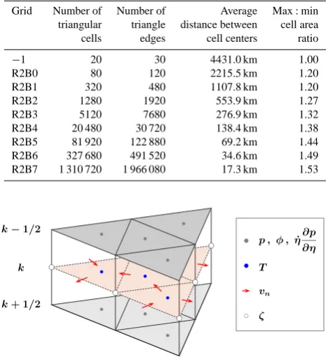
From grid level 0 onwards, only the twelve icosahedron vertices are surrounded by five triangles (they are thus also referred to as the pentagon points), while the other vertices are surrounded by six cells. This introduces irregularity into the grid, resulting in inequality in cell areas and edge lengths. Triangles closest to the pentagon points feature the most se-vere deformation. Like in Bonaventura and Ringler (2005, hereafter referred to as BR05), C-staggering is applied to the triangular cells by placing mass and temperature at triangle circumcenters. This particular choice of cell center (as op-posed to, e.g. barycenter) results in the property that the arc connecting two neighboring mass points (i.e., the dual edge) is orthogonal to and bisects the shared triangle edge. These bisection points are used as velocity points, at which the component of horizontal wind perpendicular to the edge (de-noted byvnin this paper, cf. Fig. 1) is predicted using Eq. (1).

The velocity points, however, do not bisect the dual edges due to the irregularity of the spherical grids, causing a com-ponent of first-order discretization error in the directional gradient calculated at these locations (cf. the normal gradi-ent operator defined in Sect. 4.1 and Fig. 2b). In the shallow water model the grid optimization algorithm of Heikes and Randall (1995b) was employed to reduce the off-centering (R´ıpodas et al., 2009). The Heikes-Randall optimization pro-duces more severely deformed triangular cells than on the unoptimized grid, which affects the performance of the hy-drostatic core at medium and low resolutions. Here we use the the grid optimization method of Tomita et al. (2001) for the ICOHDC which connects the triangle vertices by identi-cal linear springs of a tunable spring coefficientβ. The iter-ative optimization algorithm relocates the vertices until the spring system reaches the lowest potential energy. The re-sulting icosahedral grids feature small off-centering that de-creases with increasing resolution, moderate deformation of the triangles, and smooth transition of geometric properties throughout the horizontal domain. The parameterβ is set to

Table 1. Total number of triangle cells and edges in various grids with root divisionnr=2, the average distance between neighboring

cells, and the area ratio of largest to smallest triangles. Grid−1 is the icosahedron projected onto the sphere.

Grid Number of Number of Average Max:min triangular triangle distance between cell area cells edges cell centers ratio

−1 20 30 4431.0 km 1.00

R2B0 80 120 2215.5 km 1.20

R2B1 320 480 1107.8 km 1.20

R2B2 1280 1920 553.9 km 1.27

R2B3 5120 7680 276.9 km 1.32

R2B4 20 480 30 720 138.4 km 1.38

R2B5 81 920 122 880 69.2 km 1.44

R2B6 327 680 491 520 34.6 km 1.49

R2B7 1 310 720 1 966 080 17.3 km 1.53

k−1/2

k

k+ 1/2

p , φ , η˙_∂η∂p

T

vn

ζ

Fig. 1. Illustration of the triangular grid and the location of main variables. Vertical level indices are shown to the left of the sketch. The meaning of the symbols can be found in Sects. 2 and 3.

0.9 in this work based on inspection of the grid properties and results from dynamical core tests. Although Table 1 reveals that the area ratio of the largest to smallest cells increases with resolution, the slight loss of uniformity does not show clear impact on the testing results.

In the vertical, the widely used hybridp-σ coordinate of Simmons and Str¨ufing (1981) (“coordinate 4” in their report) is employed. The staggering follows Lorenz (1960), mean-ing that the horizontal wind and temperature are carried at “full levels” representing layer-mean values, while the verti-cal velocity is diagnosed at “half levels” (i.e. layer interfaces, cf. Fig. 1). The vertical grid is identical to that used in the ECHAM models (e.g., Roeckner et al., 2006).

4 C-grid discretization

(5)

(a)

(b)

τ

n

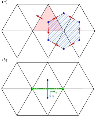
Fig. 2. Schematic showing the stencils of (a) the divergence and curl operators, and (b) the normal and tangential gradient operators described in Sect. 4.1.

4.1 Basic operators

BR05 established a spatial discretization method for solving the shallow water equations on the spherical triangular grid described in the previous section. This method forms the ba-sis for the hydrostatic model discussed here. Their discretiza-tion concept is a mimetic finite difference scheme consisting of the following elements:

– The discrete model predicts the normal component of

the horizontal windvn with respect to triangle edges.

The tangential componentvτ, needed for the vorticity

flux term in the momentum equation, is reconstructed from the normal components using vector radial basis functions (cf. references in Sect. 5.2).

– Horizontal derivatives are represented by four discrete

operators. The divergence operator div(v) applies the Gauss theorem on each triangular control volume to approximate the spatially averaged divergence over that cell (Fig. 2a). The curl operator curl(v)uses the Stokes’ theorem to approximate the vertical component of the relative vorticity averaged over a dual (hexag-onal or pentag(hexag-onal) cell centered at a triangle vertex and bounded by arcs connecting the centers of all trian-gles sharing the vertex (Fig. 2a). The directional deriva-tive of a scalar field at the midpoint of a triangle edge in the normal direction, gradn(·), is approximated by

a straightforward finite-difference discretization involv-ing two cell centers, and referred to as the (normal) gra-dient operator (Fig. 2b). The horizontal derivative tan-gential to the edge, gradτ(·), is also defined at the edge

midpoint, approximated by a central difference using values at the two ends of the edge (Fig. 2b). The mathe-matical formulations of the four operators are given by Eqs. (4), (5), (7), and (8) in BR05.

– Higher order spatial derivatives (Laplacian and

hyper-Laplacian) are constructed from the four basic opera-tors outlined above (see, e.g. Eq. 14 in Sect. 4.3). These derivatives are needed, for example, in semi-implicit time stepping schemes and for horizontal diffusion. This discretization scheme is conceptually the same as the widely used C-type discretization on quadrilateral grids. The basic operators are simple, but nevertheless have nice proper-ties. The divergence operator, essentially a finite-volume dis-cretization, makes it straightforward to achieve mass conser-vation. The curl operator guarantees that the global integral of the relative vorticity vanishes. The divergence and gradi-ent operators are mimetic in the sense that the rule of inte-gration by parts has a counterpart in the discrete model (cf. Eqs. 9 and 10 in BR05), a convenient property for achieving conservation properties. The basic operators are also highly localized (i.e. defined on small stencils), which is beneficial in massively parallel computing.

However, a question remains whether the good prop-erties of the quadrilateral C-grids in terms of the faith-ful representation of inertia-gravity waves are inherited by the triangular C-grid without limitation. For the hexago-nal/pentagonal grids (which can been viewed as the dual meshes of the triangular grids), the wave dispersion anal-ysis in Niˇckovi´c et al. (2002) revealed that discretiza-tion approaches using C-staggering could produce spurious geostrophic modes. A technique to avoid such modes on the hexagonal/pentagonal meshes was proposed in Thuburn (2008) and further developed in (Thuburn et al., 2009). On the triangular C-grids, spurious modes have also been no-ticed (e.g. Le Roux et al., 2007; Danilov, 2010; Weller et al., 2012). Some recent articles discussed this issue by analyzing the linearized shallow water equations and the representation of vector fields in a trivariate coordinate system (Thuburn, 2008; Danilov, 2010; Gassmann, 2011; Weller et al., 2012). Here, we take a different perspective and use truncation er-ror analysis to show that the divergence operator on the tri-angular C-grid described above inherently produces grid-scale checkerboard error patterns. The same analysis leads to a proposal for estimating the specific amount of numeri-cal hyper-diffusion necessary to reduce the impact of these systematic errors on numerical simulations.

4.2 Truncation error analysis

(6)

x y

o

κ1 κ2

κ3

n3 n2

n1

δ= 0

x y

o

κ1 κ2

κ3

n3 n2

n1

δ= 1

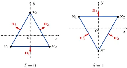
Fig. 3. Planar equilateral triangles considered in the truncation error analysis in Sect. 4.2.

then denote the normal outward unit vector at edge mid-points by nj wherej∈ [1,3]is the edge index. A label δ

is assigned to each cell to denote its orientation, with val-ues of 0 and 1 for upward- and downward-pointing trian-gles, respectively. Thus, the three neighboring cells shar-ing edges with an upward-pointshar-ing triangle are downward-pointing, and vice versa. In the truncation error calculation, a downward-pointing triangle is understood as the image of the corresponding upward-pointing triangle mirrored at the x-axis (Fig. 3). For a generic vector fieldv differentiable to a sufficiently high order, we denote its components in thex

andy directions byuandv, respectively. Applying the dis-crete divergence operator pointwise values of the vector field known at edge midpoints, denoted asvj, the 2-D Taylor

ex-pansion yields

div(v)= √

3l2

4

!−1

l 3

X

j=1

vj·nj (6)

=(∇ ·v)_o+(−1)δl H (v)o

+l

2

96

h

∇2(∇ ·v)i

o

+(−1)δl3F (v)o+O(l4) . (7)

Here the subscripto denotes the function evaluation at the triangle center. The functionsHandF read

H (v)= √

3 24 2

∂2u ∂x∂y+

∂2v ∂x2−

∂2v ∂y2

!

, (8)

F (v)= √

3 29₃3 12

∂4u ∂x3_∂y+2

∂4u ∂x∂y3+3

∂4v ∂x4

+6 ∂

4_v ∂x2_∂y2−5

∂4v ∂y4

!

. (9)

Equation (7) indicates that the discrete divergence opera-tor applied to pointwise values ofv is a first-order approx-imation of the divergence at the triangle center. More im-portantly, the first-order error term changes sign from an upward-pointing triangle to a downward-pointing one, which results in a checkerboard error pattern.

-90 -60 -30 0 30 60 90 y (degree)

0 60 120 180 240 300 360

x (degree)

-0.042 -0.021 0.000 0.021 0.042

(a) divergence error (s-1₎ _{triangular grid}

min. = -5.55E-2 max. = 5.55E-2

Fig. 4. (a) Numerical error of the cell-averaged divergence of the velocity field defined by Eq. (11), calculated using Eq. (6) on a pla-nar triangular grid with 10.4◦resolution in the x-direction. (b) The l1,l2andl∞error norms at different resolutions. The discrete diver-gence is calculated by first evaluating Eq. (11) at edge centers then applying operator (6). Numerical error is computed with respect to cell average.

In a finite-volume perspective, the divergence computed by the Gauss theorem should be interpreted as cell average rather than a pointwise value. However, it is worth noting that, in an equilateral triangle, the cell-center value can be viewed as a second-order approximation of the cell average. Therefore, the first order error term in Eq. (7) will also be present in the approximation of the cell average. Indeed, it is not difficult to check that

div(v)=(∇ ·v)c+(−1)δl H (v)o−

l2

96

h

∇2(∇ ·v)i

o

+O(l3), (10)

where()cstands for cell average. The leading error remains first order and also features a checkerboard pattern. In order to check empirically the impact of Eq. (10), numerical calcu-lations have been performed using the vector field

      

u(x, y) =1

4

r

105

2π cos 2xcos

2_y_sin_{y ,} v(x, y) = −1

2

r

15

2π cosxcosysiny ,

(7)

the divergence of which reads ∇ ·v= −1

2√2π

√

105 sin 2xcos2ysiny+ √

15 cosxcos 2y. (12) The discrete divergence is calculated by first evaluating Eq. (11) at edge centers and then applying operator (6). Nu-merical errors are calculated against the cell average given in Appendix A. Figure 4 shows the spatial distribution of the error and the convergence with respect to resolution. These results confirm the error analysis in Eq. (10).

It could also be remarked that, if the operand of the di-vergence operator is interpreted as the average along the edge rather than the point value at the edge center, then the Gauss theorem will give the exact cell-averaged diver-gence without any error. However, it should be noted that in a C-grid discretization, the divergence operator is typi-cally not applied to the horizontal velocity but to the mass flux (cf. Eqs. 3 and 4). Since the mass flux is not a prog-nostic variable but needs to be derived, an accurate edge-mean is not available. In ICON and in many other models the interpolation of density (or equivalent variables) from neighboring cells to edges gives a second order mass flux on a regular grid. It can be shown analytically that if the edge-mean mass flux is approximated tom-th order,m be-ing a positive even number, the divergence operator on an equilateral triangle will be of order m−1, and the sign of the leading error depends on the orientation of the trian-gle. (Detailed derivation can be found in Appendix B.4 of Wan (2009), available from http://www.mpimet.mpg.de/en/ science/publications/reports-on-earth-system-science.html.) In summary, the truncation error analysis shows that the divergence operator defined on the triangular C-grid yields a checkerboard error pattern. This appears to be an inherent property related to the cell shape and the placement of the ve-locity variables. The curl and gradient operators, on the other hand, are second-order accurate on the regular planar grid due to the symmetric geometry. The derivations are omitted in this paper.

Following the general procedure of studying a complex problem in a simpler but relevant context, the truncation er-ror analysis presented here is performed on a planar grid consisting equilateral triangles. In an actual model built on a spherical grid, the spherical geometry and unavoidable grid irregularity introduce more terms to the truncation error. In addition, the divergence operator operates on the discrete ve-locity field produced by model numerics which contains nu-merical error. In that case Eqs. (7) and (10) are no longer accurate. On the other hand, the key features of the triangu-lar C-grid that cause the grid-scale noise in the divergence operator, namely the asymmetric shape and the upward- and downward-pointing directions, stay unchanged.

4.3 Noise control

The checkerboard error pattern highlighted by the analysis in Sect. 4.2 enters the hydrostatic model system because of

the continuity Eq. (3) and the temperature advection term in Eq. (2) (cf. the discrete form in Sect. 5.5). Grid-scale noise in the divergence operator typically causes noise in the diver-gence field and in temperature, which then affects the veloc-ity field through the pressure gradient force. Such numerical noise, while less apparent in the barotropic tests reported in BR05 and R´ıpodas et al. (2009), significantly affects three-dimensional baroclinic simulations. One possibility to avoid this problem is to improve the divergence operator by en-larging the stencil. For example, with a four-cell stencil (one triangle plus three of its direct neighbors, involving nine ve-locity points), one can construct a second-order divergence operator on a regular grid, and apply certain measures to ap-proach second order in spherical geometry. Further discus-sions in this direction will be included in Part 2 of the paper. Here we only point out that, if the transport of tracers in the same model is to be handled by finite volume methods using a single cell as control volume, a different stencil for diver-gence in the dynamical core will destroy the tracer-and-air-mass consistency whose importance has been pointed out by, e.g. Lin and Rood (1996), J¨ockel et al. (2001), Gross et al. (2002) and Zhang et al. (2008). In this paper, we rely in-stead on a carefully chosen numerical diffusion to suppress the checkerboard noise. Although it is generally not a pre-ferred practice to use filtering or damping algorithms in nu-merical models, there is an interesting relationship between the discrete divergence and vector Laplacian on the triangu-lar C-grid that can be exploited.

As in the ICON shallow water model described in R´ıpodas et al. (2009), the vector Laplacian

∇2v= ∇(∇ ·v)− ∇ ×(∇ ×v) (13)

is approximated in an intuitive manner by

∇_d2v

e

·Ne =gradn

h

div(v)

i

−grad_τhcurl(v)

i

. (14)

Here the subscript d denotes the discrete approximation, e the edge midpoint, andNethe unit normal vector associated

to the edge. (The relationship between the unit normal vector

Ne of an edge and the outward unit vectorneof a cell that

the edge belongs to is eitherNe=neorNe= −ne.) The

no-tations div, curl, grad_n and grad_τ denote the discrete diver-gence, curl, normal gradient, and tangential gradient opera-tors defined in Sect. 4.1. The divergence operator on a regular planar grid is defined by Eq. (6) in Sect. 4.2. The fourth-order hyper-Laplacian, widely used for horizontal diffusion in at-mospheric models because of its scale selectivity, is approx-imated by

(8)

Like in the previous subsection, one can perform a Taylor expansion (but with respect to the edge midpointe) and get

∇_d4v

e

·Ne=

∇4v

e

·Ne+(−1)δ48

√

3l−2H (v)e

+O(l0) . (16)

The functionH is the same as in Eq. (7).

Assuming that the dynamical core uses a diffusion coef-ficient K4 and time step 1t, if Eq. (16) is multiplied by (−1tK4), applying the divergence operator, and retaining

only two leading terms on the right-hand side yields div−1tK4∇d4v

= −1tK4242l−3(−1)δH (v)o

−1tK4div

∇4v

o

+ · · · (17)

Now we apply Eq. (7) to the second term on the right-hand side of Eq. (17), use a symbol_Ediv,1to denote the first order

term in Eq. (7), in other words

Ediv,1=(−1)δl H (v)o, (18)

and letlˆ=l/

√

3 to denote the distance between neighboring cell centers. After some manipulation, Eq. (17) becomes div−1tK4∇d4v

o

= −1tK4

√

8/lˆ4Ediv,1

−1tK4

h

∇4(∇ ·v)i

o

+ · · · (19)

This shows that, when the vector biharmonic operator (Eq. 15) is used in the explicit numerical diffusion for hor-izontal wind, apart from the hyper diffusion one usually ex-pects (i.e. the second term on the right-hand side of Eq. 19), there is an additional effect that compensates (at least to some extent) the leading error in divergence. This additional ef-fect is similar to the divergence damping mechanism that has been adopted in many dynamical cores (e.g. Lin, 2004). Fur-thermore, if the coefficientK4is determined via a parameter τ∗using the formula

K4=

1

τ∗

ˆ

l

√

8

!4

, (20)

then1t /τ∗indicates the fraction of the checkerboard diver-gence error that can be removed after one time step.

In our numerical experiments it has been observed that the ratio1t /τ∗₌_{1 is very effective in removing the grid-scale} noise and renders a reasonably stable model configuration. Furthermore, given that the icosahedral grid is not strictly regular in terms of cell sizes and edge lengths, we use the lo-cal edge length for Eq. (20) instead of the global mean, which further improves the effectiveness of the method. Examples in the shallow water model can be found in (R´ıpodas et al., 2009).

(a)

Ac,e

cellc

edgee

(b)

||

|| ||

|

target edge

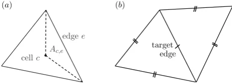
Fig. 5. (a) Schematic for the area-weighted averaging defined by Eq. (21); (b) stencil of the vector reconstruction used for obtaining the tangential velocity in Eqs. (22) and (23).

It should be mentioned, however, that this approach does have a clear disadvantage. The two terms on the right-hand side of Eq. (19) are controlled by the sameK4 coefficient.

Because the value ofK4has to be chosen to achieve a

suf-ficient compensation of the checkerboard error, there is no longer the freedom to choose the magnitude of the hyper-diffusion by physical arguments only. Since the characteris-tic damping timeτ∗corresponding to1t /τ∗=1 is consid-erably shorter than usually seen in climate models, there is a danger of overly strong diffusivity in the triangular ICO-HDC. This is in fact our major concern regarding the viabil-ity of this dynamical core in long-term climate simulations, and a point to which special attention needs to be paid in the further development.

5 Discrete formulation of the dynamical core

We introduce now the discrete form of the primitive Eqs. (1)– (4) employed in the ICOHDC.

5.1 Horizontal interpolation

On a staggered horizontal grid, the normal wind and the rela-tive vorticity are not co-located with mass (and temperature). Horizontal interpolation is thus necessary. The following in-terpolations are used in the ICOHDC:

– ψc2e, distance-based linear interpolation of a scalarψ

from two neighboring cell centers to the midpoint of the shared edge;

– ψv2e, linear interpolation of a scalarψ from two ver-tices of an edge to its midpoint (i.e. arithmetic average);

– ψe2c,lin, a bilinear interpolation from the three edges of a triangle to its circumcenter. The interpolation is per-formed in a local spherical coordinate whose equator and primal meridian intersect at the cell center;

– ψe2c,aw, an area-weighted interpolation

ψe2c,aw=X

e Ac,e

(9)

whereAc is the cell area, andAc,e the area of a

sub-triangle defined by the cell centercand the two vertices of edge e (Fig. 5a). This interpolation is constructed from the finite-volume perspective for conservation pur-poses, assuming piecewise constant sub-grid distribu-tion. Theψein Eq. (21) is assumed to represent the

av-erage value of a kite-like area whose diagonals are the edgeeand its dual.ψe2c,aw is to be understood as the average over the triangular cellc.Ac,e in Eq. (21) and

Fig. 5 is the overlapping area of cellcand the kite asso-ciated with edgee.

5.2 Vorticity flux and kinetic energy gradient

The first two terms on the right-hand side of Eq. (1), i.e. the absolute vorticity flux and the kinetic energy gradient, repre-sent the combination of horizontal momentum advection and Coriolis force in vector invariant form. The kinetic energy gradient is calculated in our model by

grad_n

0.5 v2

n+vτ2

e2c,lin

, (22)

and the absolute vorticity flux by

f+curl(v)v2evτ. (23)

As mentioned earlier, the C-grid discretization predicts only the normal component of the horizontal wind. The tangential wind vτ needed by Eqs. (22) and (23) is

recon-structed at edge midpoints using the vector radial basis func-tions (RBFs) introduced in Narcowich and Ward (1994). We use a stencil that involves four edges surrounding the tar-get edge (Fig. 5b), the inverse multi-quadric kernelψ (r)=

1/p1+(r)2, and the shape parameter=2. Test results have shown that this particular stencil used in our model is very insensitive to the choice of kernel function and shape pa-rameter. Following BR05, it is assumed that the normal and tangential components form a right-hand system. For a more detailed description and testing of this algorithm, the readers are referred to the work of Ruppert (2007) and Bonaventura et al. (2011). Here we only point out that the RBF vector reconstructions have the nice property that they allow for straightforward extension to larger stencils and higher or-der approximations, as shown, e.g., by Bonaventura et al. (2011). However, this method may have numerical issues re-lated to the ill conditioning of the interpolation matrix when the stencil is relatively large or in the case of highly irregu-lar node distribution. In those cases, enirregu-larging the shape pa-rameter can help alleviate the problem. For the reconstruc-tion of edge-based tangential velocity discussed above, be-cause of the small stencil and thanks to the quasi-regularity of the icosahedral mesh employed, the ill conditioning prob-lem does not arise. Nevertheless there are other reconstruc-tion methods available in the literature that are potentially attractive due to their mimetic properties (e.g., Perot, 2000; Thuburn et al., 2009; Wang et al., 2011).

5.3 Pressure and layer thickness

Theηcoordinate of Simmons and Str¨ufing (1981), a terrain following coordinate near the earth’s surface that gradually transforms into pressure coordinate in the upper troposphere, has been widely used in atmospheric GCMs. Here we only mention a few technical details for completeness and clarity: the pressure at layer interfaces (see Fig. 1) is given by

pk+1/2=Ak+1/2+Bk+1/2ps, k=0,1, . . . ,NLEV. (24)

Here ps stands for surface pressure. NLEV is the total number of vertical layers.AandB are predefined parame-ters (see, e.g. Roeckner et al., 2003).B=∂p/∂ps is used in Eq. (4). The pressure thickness of thek-th model layer is de-noted by1pk =pk+1/2−pk−1/2.

5.4 Continuity equation

To compute the right-hand side of Eq. (3) the divergence op-erator is applied to the mass fluxv∂p/∂η, followed by an integral through the vertical column. This discretization does not introduce any spurious sources or sinks in the total air mass, as long as the mass flux has a unique value at each edge. In this paper, the air mass flux in the normal direction

Neof an edge e is computed by

vn(∂p/∂η)

c2e

. (25)

5.5 Horizontal advection of temperature

The horizontal advection of temperature at cellcin layerkis discretized in an energy-conserving form

(v· ∇T )c,k=

1

1pc,k

div(v1p T )c,k−Tc,kdiv(v1p)c,k

.

(26) The mass flux divergence in this equation is the same as in the discrete continuity equation. The heat flux divergence is cal-culated by first interpolating temperature and layer thickness separately from cells to edges using the distance-based linear interpolation, multiplying by the normal wind, and then ap-plying the discrete divergence operator. Because of the rather simple flux calculation and the inherent property of the diver-gence operator discussed earlier, the temperature advection is only first-order accurate. The limitation of this low-order scheme is discussed in Sect. 6.1.2.

5.6 Vertical advection of momentum and temperature

(10)

and Burridge (1981, hereafter SB81): ˙ η∂ψ ∂η k = ˙ η∂p ∂η ∂ψ ∂p k = 1

21pk

( ˙ η∂p ∂η

k+1/2

(ψk+1−ψk)

+ ˙ η∂p ∂η

k−1/2

(ψk−ψk−1)

)

. (27)

Hereψ is either temperature or a horizontal wind compo-nent. The vertical indices are illustrated in Fig. 1. The ver-tical velocities at layer interfaces are diagnosed by Eq. (4). Note that Eq. (27) can be derived by applying the idea of Eq. (26) to the vertical direction, then replacing the diver-gence operator by the central difference, and the cell-to-edge interpolation by the arithmetic average.

For the advection of the normal wind in the ICOHDC, Eq. (27) requires layer thickness and vertical velocity at edge midpoints. These are obtained by the linear interpolation mentioned earlier in Sect. 5.4.

5.7 Hydrostatic equation

The hydrostatic equation involves only vertical discretiza-tion, thus takes the same form in the ICOHDC as in SB81 and in the spectral core of ECHAM. The discrete counterpart of Eq. (5) reads

φc,k+1/2=φc,s+

NLEV

X

j=k+1

RdTc,jln

_pc

,j+1/2 pc,j−1/2

(28)

for layer interfaces withk_>1. Hereφc,sdenotes the surface

geopotential at cell c. The geopotential at full levels are given by

φc,k=φc,k+1/2+αc,kRdTc,k (29)

where

αc,k=

(

ln 2, fork=1;

1−pc,k−1/2 1pc,k ln

_p

c,k+1/2

pc,k−1/2

, fork >1. (30) 5.8 Pressure gradient force and adiabatic heating

After computing the geopotential by Eq. (29), the last term in the velocity Eq. (1) can be obtained by applying the normal gradient operator.

The pressure gradient term in the same equation is calcu-lated by

(RdT∇lnp)e·Ne= RdT

c2e

grad_n

_p

k+1/2lnpk+1/2−pk−1/2lnpk−1/2 1pk

. (31)

Using Eq. (31), the first part of the adiabatic heating term in the temperature equation (2) can be obtained by

RdT

p v· ∇p

c,k

= 2vn1p[(RdT∇lnp)·Ne]

e2c,aw

1pc,k

.

(32) The remaining part is approximated by

_R

dT

p

_∂p

∂t + ˙η ∂p ∂η

c,k =

−RdTc,k

1pc,k

"

ln

_p

c,k+1/2 pc,k−1/2

k−1 X

j=1

div(v1p)_c_,j

+αc,kdiv(v1p)c,k

. (33)

Both Eqs. (32) and (33) are derived following the energy con-servation constraint in SB81.

5.9 A few remarks on the spatial discretization

In this section we have mentioned repeatedly the C-grid dis-cretization of SB81, which is an energy-conserving scheme on regular latitude-longitude grids, designed for an early finite-difference version of the NWP model of the European Centre for Medium-range Weather Forecasts. In the base-line version of the ICOHDC, the kinetic energy gradient and the absolute vorticity flux discretized on the triangular grid (Eqs. 22 and 23) do not guarantee energy conservation to ma-chine precision, partly due to the tangential wind reconstruc-tion using the RBFs. The other discrete formulae described in Sects. 5.4–5.8, on the other hand, do help avoid spurious energy sources/sinks.

Potentially, there might be another issue related to the RBF reconstruction. As discussed in Hollingsworth et al. (1983) and Gassmann (2013), certain inconsistencies between the discrete vorticity flux and kinetic energy gradient can trig-ger nonlinear instability that manifests itself as small-scale noise at high resolutions. So far we have not seen clear evi-dences of such instability in the test results of the ICOHDC (cf. Sect. 6).

5.10 Time stepping scheme

(11)

associated with phase speed higher than 30 m s−1_are

numer-ically solved using the generalized minimal residual method (GMRES, Saad and Schultz, 1986).

In the standard model configuration, the time stepping scheme uses the following parameters: the Asselin coeffi-cient is 0.1 following ECHAM. In the semi-implicit correc-tion, coefficients of the gravity wave terms evaluated at the old and new time steps are set to 0.3 and 0.7, respectively, following the global forecast model GME of the German Weather Service (Majewski et al., 2002). Detailed formula-tion of the time integraformula-tion algorithm is given in Appendix B. As mentioned earlier in the introduction, this particular time stepping scheme is used here for the sake of a clean eval-uation of the spatial discretization employed on the triangular icosahedral grids. The GMRES solver is chosen for its reli-ability and streli-ability, since this is one of the standard solvers for large non-symmetric linear systems. Issues arising in par-allel versions of this algorithm have been discussed in the literature by, e.g., de Sturler and van der Vorst (1995). In massively parallel simulations, especially when the dynami-cal core consumes a significant portion of the total comput-ing time, linear solvers that require global communications will pose constraints on the computational performance. In such cases, explicit time stepping schemes are an option to consider. For example, the ICON nonhydrostatic model uses a two-time-level predictor-corrector scheme, with im-plicit treatment restricted to the vertically propagating sound waves. In the ICOHDC, we have implemented various ex-plicit or semi-imex-plicit two-time-level integration schemes for the purpose of achieving tracer-and-air-mass consistency, but these are considered beyond the scope of the baseline model.

5.11 Tracer transport

A group of upwind, conservative, flux-form semi-Lagrangian transport algorithms are implemented for tracer transport in the ICON triangular models. Options for horizontal advec-tion include the first-order upwind scheme, and a triangu-lar version of the “swept-area” approach following Miura (2007). The latter algorithm is second-order in time and ei-ther second-, third- or fourth-order in space, depending on the choice of reconstruction polynomial (linear, quadratic or cubic). The polynomial coefficients are estimated using a conservative weighted least squares reconstruction method (Ollivier-Gooch and Altena, 2002). Transport in the ver-tical is calculated with the Piecewise Parabolic Method (PPM, third-order, Colella and Woodward, 1984). The op-tional limiters employed include semi-monotonic and mono-tonic slope limiters (Barth and Jespersen, 1989) as well as the Flux Corrected Transport approach (FCT, Zalesak, 1979). Consistency between tracer transport and the dis-crete continuity equation can be achieved when the dy-namical core uses a two-time-level time stepping scheme. These transport algorithms in the ICON models have gone through comprehensive testing, e.g., following the proposal

of Lauritzen et al. (2012b). Some of the evaluation results are presented in http://www.cgd.ucar.edu/cms/pel/transport-workshop/2011/16-Reinert.pdf. More detailed results of the second-order (linear) horizontal transport can be found in Lauritzen et al., (2013)1.

In the present version of the ICOHDC, the discretization of horizontal temperature advection does not yet make use of the semi-Lagrangian transport schemes, but is calculated using Eq. (26) with a rather crude approximation of the heat flux at triangle edges (Sect. 5.5). The limitation of the lat-ter scheme is discussed in Sect. 6.1.2. In the nonhydrostatic dynamical core Z¨angl et al. (2013), horizontal advection in the thermodynamic equation and the continuity equation is discretized using the edge-based potential temperature and density values estimated with the second-order Miura (2007) scheme.

6 Idealized dry dynamical core tests

In this section we present results of numerical simulations carried out to evaluate the new dynamical core. The goal here is to find out whether the present version of the ICO-HDC can correctly represent basic processes of the adiabatic atmospheric dynamics, and to analyze the sensitivity of the numerical solutions to horizontal resolution. During the de-velopment of the new model, we routinely perform a suite of idealized dry dynamical core tests with different levels of complexity. The simplest ones are 3-D extensions of the widely used shallow water tests 5 and 6 from Williamson et al. (1992). The barotropic cases are in some sense a sanity check for the 3-D formulation of the ICOHDC and its prac-tical implementation in the code. These results can be found in Wan (2009), and are not repeated here. This section fo-cuses on two deterministic baroclinic tests (Sect. 6.1) and an idealized dry “climate” test (Sect. 6.2).

Here we want to make the remark that model evaluation and inter-comparison is a delicate matter. Due to the com-plexity of the governing equations, the wide spectrum of dy-namical regimes and waves that they support, and the vari-ous components that constitute (and affect the properties of) a discrete model, it is very difficult, if possible at all, to se-lect one single metric to summarize the model performance. In this section, especially in the baroclinic wave test, we carry out simulations with both the ICOHDC and the spec-tral transform dynamical core of ECHAM at multiple resolu-tions, and compare the results in several ways including qual-itative comparisons, difference norms, and dispersion errors. We think this collection of numerical results provides useful information for the climate and weather modelers who face

1_{Lauritzen, P. H. et al. (2013): A standard test case suite for}

(12)

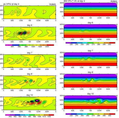
Fig. 6. Evolution of the baroclinic wave in the Jablonowski and Williamson (2006a,b) test case, as shown by the surface pressure (unit: hPa, left column) and 850 hPa temperature (unit: K, right column) simulated by the new dynamical core at R2B5 (70 km) resolution. Note that in the left column, the two upper panels use a different color scale than the lower panels. Further details can be found in Sect. 6.1.2.

the question of which numerical method better suits their needs and expectations.

All ICOHDC results presented in this section are obtained using revision 6489 of the model code. The vertical grid is fixed at L31, which resolves the atmosphere from the surface to 10 hPa, as commonly used in the tropospheric version of the ECHAM model (e.g., Roeckner et al., 2006). The model time step is set to 600 s at R2B4, and reduced by half when the grid level is increased by one.

6.1 Deterministic baroclinic tests

The test case proposed by Jablonowski and Williamson (2006a,b, hereafter JW06) has been widely used in recent years for testing 3-D atmospheric dynamical cores. Inspired by the baroclinic instability theory, the deterministic test

con-sists of two parts: a steady state test followed by a baroclinic instability test.

6.1.1 Steady state test

(13)

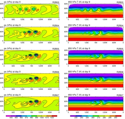
Fig. 7. Surface pressure (unit: hPa, left column) and 850 hPa temperature (unit: K, right column) at day 9 in the Jablonowski and Williamson (2006a,b) baroclinic wave test simulated by the new dynamical core at various horizontal resolutions. Further details can be found in Sect. 6.1.2.

near the pentagon points (cf. Sect. 3), resulting in wavenum-ber 5 patterns near 26.6◦N/S. Embedded in the dynamically unstable mean state of this test case, the perturbations am-plify for more than 10 days, then reach a quasi-equilibrium state after 20 to 30 days (not shown). As the horizontal reso-lution increases, the magnitude of the numerical errors is re-duced and the perturbations evolve less rapidly. These behav-iors agree with our expectation, and are similar to the results of the GME model (also built on icosahedral grids) presented in JW06.

6.1.2 Baroclinic wave test

The second part of this test case focuses on the evolution of an idealized baroclinic wave in the Northern Hemisphere, triggered by an analytically specified large-scale perturba-tion in the wind field. Cyclone-like structures develop in the

course of about 10 days, featuring lows and highs in the sur-face pressure field (Fig. 6, left column) and accompanying fronts in the lower troposphere temperature (Fig. 6, right col-umn). This figure shows the ICOHDC simulation at R2B5 resolution which has an average grid spacing of 70 km be-tween neighboring mass points. The key features of the sim-ulated baroclinic wave evolution, including the slow devel-opment of the perturbations in the first 6 days and the subse-quent exponential intensification, as well as the magnitude of the closed cells in surface pressure and the fronts in tempera-ture, agree well with the reference solutions given by JW06.

(a) Convergence

(14)

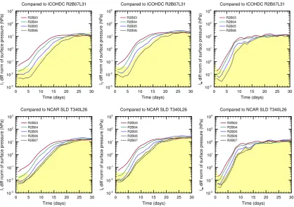
Fig. 8.l1,l2andl∞norms (left, middle and right columns, respectively) of surface pressure differences (unit: hPa) in the Jablonowski and Williamson (2006a,b) baroclinic wave test between lower-resolution ICOHDC simulations and the R2B7 solution (upper row), and between all ICOHDC simulations shown in Fig. 7 and the NCAR semi-Lagrangian model result at T340 resolution (lower row). Further details can be found in Sect. 6.1.2.

(at R2B3) to 17.5 km (at R2B7). The solution obtained on the coarsest grid (R2B3) is of unsatisfactory quality, in that the depressions are too weak, while the spurious perturbations at the rear of the wave train are too strong. This resolution is thus not recommended for future applications of the new dynamical core. The next solution, at R2B4, is significantly improved, although the first two low pressure cells are still somewhat weak, and there is an easily detectable phase lag in the propagation of the wave in comparison with the solu-tion at R2B7. As the grid is further refined, the phase lag gets smaller, and the depressions become deeper. The two runs at the highest resolutions (R2B6 and R2B7) look very similar, and are hardly distinguishable from the reference solutions in JW06 by visual comparison.

To quantitatively assess the convergence of these numer-ical solutions, we follow JW06 and use the l1, l2 and l∞ differences norms of surface pressure as the metric. In the work of JW06 it was found that differences among solutions from four models using very different discretization methods stopped decreasing once the resolutions increased beyond a certain limit. Based on this observation, the uncertainty in their reference solutions was estimated. The corresponding uncertainties in the difference norms are shown by the

yel-low shading in Fig. 8. When the difference norms fall beyel-low the uncertainty limit, the solution being tested is considered as having the same quality as the reference solution.

In Fig. 8 the norms ofps differences are shown between the R2B3 to R2B6 simulations and the R2B7 run (upper row), as well as between the ICOHDC simulations and a ref-erence solution in JW06 from the National Center for Atmo-spheric Research Semi-Lagrangian dynamical core (NCAR SLD, Fig. 8 second row). Difference norms computed against the other reference solutions in JW06 are very similar hence not shown. Regardless of the choice of reference, panels in Fig. 8 clearly indicate a decrease in the difference norms when the horizontal resolution increases. Convergence of the numerical solution is achieved at R2B6. The R2B6 and R2B7 solutions are able to represent the baroclinic wave evolution within the uncertainty in the reference solution.

(b) Phase speed

(15)

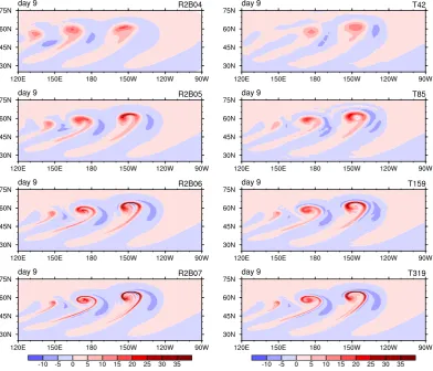
Fig. 9. 850 hPa relative vorticity (unit: 10−5s−1) at day 9 in the Jablonowski and Williamson (2006a,b) baroclinic instability test simulated by the new dynamical core (left column) and the spectral transform core of ECHAM (right column) at various horizontal resolutions. Further details can be found in Sect. 6.1.2.

Fig. 10. As in Fig. 8 but between simulations performed with the spectral transform dynamical core of ECHAM and the reference solution at T340 provided by the NCAR semi-Lagrangian model.

comparing the strength of the vortices, the magnitude of the horizontal gradients, and the level of details of the character-istic patterns represented by the models in Fig. 9, we find that

(16)

Table 2. Resolutions of the ICOHDC and the spectral core of ECHAM that produce similar results in the baroclinic wave test case. The grid size given in the left half of the table is the average distance between mass points on the triangular grids. “dx” in the right half of the table refers to the zonal spacing of the Gauss grid. The degrees of freedom (DOF) and the total number of mass pointsnMare included in the table

for the discussion in Appendix C. The DOF of the ICOHDC is defined as the total number of velocity and mass (temperature) points on one vertical level. The DOF of the spectral core is defined as the total number of spectral coefficients of vorticity, divergence, and temperature on one vertical level. ThenMin the spectral model is that of the corresponding Gauss grid.

ICOHDC Spectral core of ECHAM

Grid Name Grid Size DOF nM Truncation dxat 60◦N dxat Equator DOF nM

R2B4 138.5 km 51 200 20 480 (T51) 128.3 km 256.6 km 8268 12 168

R5B3 110.8 km 80 000 32 000 T63 104.3 km 208.5 km 12 480 18 432

R3B4 92.3 km 115 200 46 080 (T76) 86.3 km 172.5 km 18 018 26 912

R2B5 69.2 km 204 800 81 920 T106 62.6 km 125.1 km 34 668 51 200

R5B4 55.4 km 320 000 128 000 T127 52.1 km 104.3 km 49 536 73 728

R3B5 46.2 km 460 800 184 320 (T151) 43.9 km 87.8 km 69 768 103 968

R2B6 34.6 km 819 200 327 680 (T213) 31.3 km 62.5 km 138 030 204 800

R5B5 27.7 km 1 280 000 512 000 T255 26.1 km 52.1 km 197 376 294 912

R3B6 23.1 km 1 843 200 737 280 (T302) 22.0 km 44.1 km 276 336 412 232

R2B7 17.3 km 3 276 800 1 310 720 (T403) 16.5 km 33.0 km 490 860 734 472

R2B5 are stronger than those of T85 (Fig. 9, third row), the T85 simulation captures the reference solution within the un-certainty while R2B5 does not. According to the snapshots, the errors in the lower-resolution spectral model results are mainly in the strength of the vortices and the spatial gradi-ents, while in the ICOHDC the phase speed is also a major source of numerical error.

Phase error is a typical problem associated with dynami-cal cores using second (or lower) order spatial discretization methods. It is also one of the main disadvantages of such models at medium and low resolutions in comparison with the spectral transform method. It is worth noting that in JW06 the finite-difference model GME has a similar phase prob-lem, while the NCAR finite volume core (Lin, 2004), which uses the third-order piecewise parabolic advection algorithm, does not. Skamarock and Gassmann (2011) showed that in their models, replacing the second-order potential tempera-ture transport by third-order schemes can significantly reduce the magnitude of the phase error in this test case and sup-press its growth. In the hydrostatic dynamical core discussed here, horizontal temperature advection is computed using the first-order scheme described in Sect. 5.5. A higher-order dis-cretization, e.g., using the transport algorithms outlined in Sect. 5.11, will probably help to improve the solution quality at R2B5 and lower resolutions. On the other hand, Fig. 9 also suggests that phase error in the ICOHDC becomes negligible at R2B6 (35 km). Since the ICON models are developed for high-resolution modelling, the phase error is not expected to be an obstacle in those applications of the new model system.

(c) Equivalent resolution in terms of solution quality

Since the ultimate purpose of developing the new ICON models is to use them in operational NWP and climate

appli-cations, a natural question one would expect from the poten-tial users, especially from those having been using ECHAM, is the equivalent resolutions between the ICOHDC and the spectral core in terms of solution quality. For reasons dis-cussed in detail in Appendix C, we believe such relation-ships are difficult to identify a priori, but rather need to be established by comparing results from numerical tests. This is in line with, e.g., the work of Williamson (2008a) who discussed the equivalent resolutions between a finite-volume model and a spectral transform model.

Baroclinic wave tests are carried out with the icosahedral grids listed in the left half of Table 2, and at the spectral trun-cations given without parenthesis in the right half of the table. Qualitative comparison as in Fig. 9 is used to identify reso-lution pairs (R5B3, T63), (R2B5, T106), etc., that produce similar results. It turns out that for these visually identified pairs, the ratios between the average grid spacing of differ-ent icosahedral grids match well with the ratios between the corresponding truncation wavenumbers. We then use this re-lationship to derive the wavenumbers given in parenthesis, which are not “standard” resolutions of the ECHAM model. In principle it would be useful to verify the established equivalent resolutions in some quantitative manner, for ex-ample by calculating the difference norms of surface pressure in each pair, and comparing them with the uncertainty esti-mates (the yellow shading in Figs. 8 and 10). At the current stage, however, the difference norms between the medium-and low-resolution pairs would lie outside the uncertainty range unless the phase error in the ICOHDC was reduced. The verification is thus not done in this study.

(17)

resolution. This is probably not a coincidence, but a result of the fact that in this test case the baroclinic wave evolves and propagates near this latitude. Nonlinear terms in the primi-tive equations play a crucial role in the baroclinic instabil-ity development. In both models these terms are computed in grid-point space using similar discretization schemes fol-lowing the work of SB81. It is thus not surprising that the equivalent resolutions we identified turn out to have similar spacing at 60◦N. In a different test case that features dynam-ical processes confined to, say, the tropics, the conclusions on equivalent resolutions may be different.

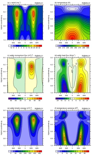
6.2 Held–Suarez test

After the adiabatic deterministic test cases discussed above, we consider here the dry “climate” experiment proposed by Held and Suarez (1994), in which the dynamical core is forced by Rayleigh damping of horizontal wind in the near-surface layers as well as relaxation of the temperature field towards a prescribed, north–south and zonally symmetric ra-diative equilibrium. The original goal of this popular test was to evaluate the zonal-mean climatology obtained from the last 1000 days of a 1200 day simulation. However, a more comprehensive analysis of the inherent low-frequency vari-ability was carried out in Wan et al. (2008), where an ensem-ble approach was proposed for the evaluation of the results. Here we follow this approach and perform ensembles con-sisting of 10 independent 300 day integrations. Each integra-tion starts from the JW06 zonally symmetric initial condiintegra-tion with random noise of magnitude 1 m s−1 added to the wind field. (This choice is rather arbitrary. As long as the 10 inte-grations within an ensemble are independent, the conclusions drawn in this subsection are not affected by the initial condi-tion.) Simulations are performed at resolutions R2B3, R2B4 and R2B5 using the same configurations as in the determin-istic test cases. The zonal-mean climate states are diagnosed from the last 100 days of each integration.

Figure 11 presents the ensemble mean model climate at R2B5. Although simple by design, the Held–Suarez test is able to reproduce many realistic features of the global cir-culation. Baroclinic eddies cause strong poleward heat and momentum transport (Fig. 11d and c, respectively). The heat transport reduces the meridional temperature gradient in comparison to the prescribed radiative equilibrium (Fig. 11b, here in comparison to Fig. 1c in Held and Suarez, 1994). The meridional transport of angular momentum converges in the mid-latitudes, forming a single westerly jet in each hemi-sphere (Fig. 11a). The core regions of the jets are located near 250 hPa. The maximum time- and zonal-mean zonal wind is about 30 m s−1. Easterlies appear in the equatorial and polar lower atmosphere, as well as in the tropics near the model top. The baroclinic wave activities concentrate in the mid-latitudes, as depicted by the transient eddy kinetic energy and temperature variance (Fig. 11e and f). The single maximum of eddy kinetic energy in each hemisphere appears in the

up-per troposphere near 45◦_{latitude, close to the core region of} the westerly jet. Easterlies in the tropics show little variance. In each hemisphere, the maximum temperature variance ap-pears near the earth’s surface and extends upward and pole-ward. A second maximum of smaller magnitude occurs near the tropopause. These features of the simulated circulation agree well with results reported in the literature (e.g. Held and Suarez, 1994; Jablonowski, 1998; Lin, 2004; Wan et al., 2008).

Sensitivity of the ICOHDC results to horizontal resolu-tion is revealed by Figs. 12 and 13. The contour lines show the differences in the ensemble average of the quantities displayed in Fig. 11, while the gray and light-blue shad-ings indicate where the differences are significant (at 0.05 and 0.01 significance levels, respectively) according to the Kolmogorov–Smirnov test (Press et al., 1992). Comparing R2B3 with R2B5, the increase in horizontal resolution leads to a substantial enhancement of the eddy activity in the mid-latitudes, stronger poleward transport, and consequently higher temperature in the Polar Regions as well as a pole-ward shift of the westerly jets. The differences between the R2B4 and R2B5 ensembles are much smaller (Figs. 13). Although one can still see enhancement in the eddy activ-ities (Fig. 13d–f) and temperature differences in high alti-tudes/latitudes regions (Fig. 13b), the discrepancies are gen-erally much smaller than between R2B3 and R2B5. Fig-ures 12 and 13 together show a clear trend of convergence in the ICOHDC results.

7 First results from the aqua-planet experiments

In the previous section we have evaluated the ICOHDC us-ing dry dynamical core tests at various resolutions. On the whole, the new core produces results that agree reasonably well with those from the spectral core of ECHAM, as well as with the reference solutions available in the literature. In these test cases, the grid-scale noise discussed in Sect. 4 is effectively suppressed and has not yet brought obvious detri-mental effects. One might argue that when moist processes are included in the model, condensational heating will act as a positive feedback, which will amplify the grid-scale noise and make the model unstable. To find out whether this is the case, we perform aqua-planet simulations following the pro-posal of Neale and Hoskins (2000).

(18)

Fig. 11. Zonal mean climate state simulated by the ICOHDC in the Held–Suarez test at R2B5 resolution. The quantities shown are ensemble averages of 10 independent integrations. Each ensemble member starts from the same initial condition but with random noise added to the wind field. Further details can be found in Sect. 6.2.

is performed every other hour as in ECHAM. The large-scale horizontal transport of water vapor, cloud liquid and cloud ice is computed using the second-order Miura (2007) scheme with monotonic FCT, while the vertical transport uses the

(19)

Fig. 12. Differences between the ensemble mean climate statistics in the Held–Suarez tests performed with the ICOHDC at R2B3 and R2B5 resolutions. Dashed contours indicate negative values. In the areas with gray and light blue shading, the differences are judged to be significant in the Kolmogorov–Smirnov test at 0.05 and 0.01 significance levels, respectively. Further details can be found in Sect. 6.2.

Simulations are performed at R2B4 using the “Con-trol” and “Qobs” sea surface temperature (SST) profiles of Neale and Hoskins (2000). The reference solutions are from

(20)

Fig. 13. As in Fig. 12 but for the differences between R2B4 and R2B5 simulations.

Here we do not attempt to investigate the convergence of the aqua-planet experiments (APE) from either ICOHAM or ECHAM6, because both models are new, and neither has been tuned at many resolutions. The intention here is rather to have a first look at the main features of the model

(21)

Fig. 14. Time and zonal mean surface precipitation rate (unit: mm day−1, solid black lines) simulated by ICOHAM in aqua-planet simulations at R2B4L31 resolution using the “Control” (left) and “Qobs” (right) SST profiles. The contributions from convective (dotted red lines) and large-scale (dashed blue lines) precipitation are also displayed. Further details can be found in Sect. 7.