www.geosci-model-dev.net/7/737/2014/ doi:10.5194/gmd-7-737-2014
© Author(s) 2014. CC Attribution 3.0 License.
Geoscientific
Model Development
Application and evaluation of a new radiation code under McICA
scheme in BCC_AGCM2.0.1
H. Zhang1,2, X. Jing1,2, and J. Li3
1Laboratory for Climate Studies, National Climate Center, China Meteorological Administration, Beijing, China
2Collaborative Innovation Center on Forecast and Evaluation of Meteorological Disasters, Nanjing University of Information Science & Technology, Nanjing, China
3Canadian Center for Climate Modeling and Analysis, University of Victoria, Victoria, British Columbia, Canada
Correspondence to: H. Zhang ([email protected])
Received: 26 July 2013 – Published in Geosci. Model Dev. Discuss.: 16 September 2013 Revised: 10 March 2014 – Accepted: 10 March 2014 – Published: 6 May 2014
Abstract. This research incorporates the correlatedk distri-bution BCC-RAD radiation model into the climate model BCC_AGCM2.0.1 and examines the change in climate sim-ulation by implementation of the new radiation algorithm. It is shown that both clear-sky radiation fluxes and cloud radia-tive forcings (CRFs) are improved. The modeled atmospheric temperature and specific humidity are also improved due to changes in radiative heating rates, which most likely stem from the revised treatment of gaseous absorption.
Subgrid cloud variability, including vertical overlap of fractional clouds and horizontal inhomogeneity in cloud con-densate, is addressed by using the Monte Carlo Indepen-dent Column Approximation (McICA) method. In McICA, a cloud-type-dependent function for cloud fraction decorre-lation length, which gives zonal mean results very close to the observations of CloudSat/CALIPSO, is developed. Com-pared to utilizing a globally constant decorrelation length, the maximum changes in seasonal CRFs by the new scheme can be as large as 10 and 20 W m−2for longwave (LW) and short-wave (SW) CRFs, respectively, mostly located in the tropics. The inclusion of an observation-based horizontal inhomo-geneity of cloud condensate has also a significant impact on CRFs, with global means of∼1.5 W m−2and∼3.7 Wm−2 for LW and SW CRFs at the top of atmosphere (TOA), re-spectively. Generally, incorporating McICA and horizontal inhomogeneity of cloud condensate in the BCC-RAD model reduces global mean TOA and surface SW and LW flux bi-ases in BCC_AGCM2.0.1.
These results demonstrate the feasibility of the new model configuration to be used in BCC_AGCM2.0.1 for climate
simulations, and also indicate that more detailed real-world information on cloud structures should be obtained to con-strain cloud settings in McICA in the future.
1 Introduction
How to deal with cloud vertical overlap and cloud internal inhomogeneity has been a very difficult task for atmospheric radiation. This arises mostly from the relatively coarse spa-tial resolution of GCMs (dozens to hundreds of kilometers), which leaves cloud-relevant processes and inherent subgrid variations of clouds unresolved (Barker and Räisänen, 2005; Zhang et al., 2013). Typically, cloud condensate (water and ice) is treated as horizontally homogeneous (the plane paral-lel homogeneous, or PPH, assumption) within a GCM grid cell. Additionally, certain predetermined assumptions about the vertical overlap of fractional clouds are required (tra-ditionally maximum-random overlap, or MRO) (Tian and Curry, 1989). Computing on a cloud system resolving model (CSRM) data set, Barker and Räisänen (2005) found that, by a small change to the standard deviation of cloud con-densate distribution, zonal mean shortwave (SW) cloud ra-diative forcing (CRF) could change up to 25 W m−2 at cer-tain latitudes (with a global mean of∼8 W m−2). The radia-tive sensitivity to cloud overlap is of similar magnitude for global averages. Oreopoulos et al. (2012) included a beta dis-tribution function and a latitude-/day-dependent cloud over-lap function, both derived from CloudSat/CALIPSO data, in the GEOS-5 atmospheric general circulation model. SW and longwave (LW) CRFs showed significant changes compared to the traditional PPH and maximum-random overlap setup, but the magnitude of changes depends also on the cloud scheme utilized. All of these studies have emphasized the importance of faithfully addressing subgrid cloud variability in GCMs.
To make the representation of subgrid cloud properties flexible and modularized and to maintain computational ef-ficiency, a scheme named the Monte Carlo Independent Column Approximation (McICA) method was developed (Pincus et al., 2003). McICA is a method that does fast spec-tral integration over given cloudy subcolumns within a do-main. The cloud subcolumns required by McICA can be sup-plied from certain subgrid cloud generators (Räisänen and Barker, 2004) or cloud-resolving models (Hill et al., 2011). The advantages of McICA are that it facilitates adjustment or alteration of both cloud structure and radiative transfer and thus accelerates future development of GCMs.
Though McICA has been extensively studied, there lacks a detailed description on cloud-type-related vertical over-lap. An e-folding relationship of cloud overlap has been de-veloped to quantitatively represent cloud overlap for differ-ent types of clouds and over differdiffer-ent regions (Hogan and Illingworth, 2000; Mace and Benson-Troth, 2002). In cur-rent GCMs, a global mean constant value of decorrelation length (hereinafter Lcf), a critical parameter in this over-lap algorithm, is often used. Usually, convective cloud has well-organized structures with large vertical correlation due to strong upward motion. Therefore,Lcffor convective cloud should be larger than for the other types of clouds. To address the climate impact by distinguishing the cloud-type-related
Lcfin McICA is one goal of this work. We here incorporate
the McICA scheme and a stochastic cloud generator (SCG; Räisänen et al., 2004) into the BCC_AGCM2.0.1 model with the BCC-RAD radiation algorithm.
This work contains two parts: first, we report the improve-ments on climate simulation by introducing the new BCC-RAD radiation algorithm. Second, we analyze the impact of cloud overlap assumption and cloud condensate inhomo-geneity through the McICA scheme. Most attention will be paid to the cloud-type-related decorrelation length by com-paring with the results of using a globally constant value. This preliminary work aims to document the impact of the modifications in cloud-radiation process on simulated cli-mate and the model response to these changes and thereby provide suggestions for future development. In Sect. 2, the BCC_AGCM2.0.1 model, the BCC-RAD radiation scheme and the McICA scheme are briefly described. The design of experiments is given in Sect. 3. Results of the simulations with various model configurations are described in Sect. 4. In Sect. 5, we conclude with a brief summary.
2 Model description
2.1 Description of BCC_AGCM2.0.1
BCC_AGCM2.0.1 was developed by the Beijing Climate Center (BCC) at the China Meteorological Administration (CMA) based on the Community Atmosphere Model Version 3 (CAM3) of the National Center for Atmospheric Research (NCAR) (Wu et al., 2010). The model runs at T42 spectral resolution (approximately 2.8◦×2.8◦) horizontally, and it
uses vertical hybridδ-pressure coordinates including 26 lay-ers with the top located at about 2.9 hPa. An additional layer is added above the topmost layer in the radiative calculation to prevent excessive heating. The default timestep is 20 min, and the radiation code is invoked every three timesteps.
Table 1. Comparison of the new and old schemes.
Old New
Absorbing gases in LW H2O, CO2, and O3
CH4, N2O, CFC11, CFC12
The same as in Old
Absorbing gases in SW H2O, CO2, O3, and O2 H2O, CO2, O3, N2O, and O2
Range of LW 0–2000 cm−1 0–2680 cm−1
Range of SW 2000–50 000 cm−1 2110–49 000 cm−1,∗ Band transmittance scheme Band model (LW: Kiehl and Briegleb, 1991)
(SW: Briegleb, 1992)
CKD scheme (Zhang et al., 2003, 2006a, b)
RT solver in LW Absorptivity/emissivity formulations (Ramanathan and Downey, 1986)
Two-stream approximation (Nakajima et al., 2000)
RT solver in SW δ-Eddington method (Briegleb, 1992) δ-Eddington method (Coakley et al., 1983) Cloud fraction parameterization Diagnostic scheme (Rasch and Kristjansson,
1998)
The same as in Old
Cloud optics LW: emissivity formulations (Ebert and Curry, 1992); SW: formulas of Slingo (1989) for liquid and of Ebert and Curry (1992) for ice
Ice cloud: computed using data from Fu (1996), Yang et al. (2005), and Hong et al. (2009); liquid cloud: Nakajima et al. (2000) Cloud effective radius Ice cloud: Kristjansson et al. (2000); Liquid
cloud: Kiehl et al. (1994)
Ice cloud: Wyser (1998); Liquid cloud: the same as in Old
Cloud overlap Maximum random overlap (MRO) (Collins, 2001)
McICA (Räisänen and Barker, 2004; Barker et al., 2008)
Aerosol–radiation coupling scheme BCC_AGCM2.0.1_CAM (Zhang et al., 2012) BCC_AGCM2.0.1_CAM (Zhang et al., 2012)
∗In the new scheme, contributions from the solar spectrum and terrestrial emission are mixed within 2110–2680 cm−1.
2.2 Description of radiation schemes
In this work, we incorporate the CKD model by Zhang et al. (2003, 2006a, b), i.e., the Beijing Climate Center Radi-ation transfer model (BCC-RAD), into BCC_AGCM2.0.1. The BCC-RAD model is substantially different from the pre-vious radiation scheme used in BCC_AGCM2.0.1. To ex-plain the importance of this radiation scheme in modulating climate simulation, it is necessary to describe this revision in advance. A detailed comparison between the old and new schemes is provided in Table 1.
The previous radiation scheme in BCC_AGCM2.0.1 is ba-sically a band model. Although some band models simu-lated well the broadband fluxes and heating rates, this may have been partly fortuitous because of band overlap effects (Ellington et al., 1991). Another defect of band models is the use of a scaling procedure to account for inhomogeneous atmospheric paths, although these can be made arbitrarily ac-curate for a homogeneous atmosphere (Kratz, 1995). There-fore, there has been a trend over the past decades to replace band models with CKD methods in GCMs.
The 10–49 000 cm−1 (0.204–1000 µm) spectral range in BCC-RAD is divided into 17 bands (8 LW and 9 SW). Five major greenhouse gases (GHGs) – H2O, CO2, O3, N2O, and CH4 – as well as chlorofluorocarbons (CFCs) are consid-ered. The major absorbers in the solar bands are H2O (in-cluding continuum absorption), CO2, N2O, O3, and O2. The HITRAN2000 database (Rothman et al., 2003) was used to provide line parameters and cross sections. Lu et al. (2012)
compared the line parameters in different HITRAN versions and found that the difference in the simulated radiative fluxes between the updated HITRAN2008 and HITRAN2000 is very small, so the use of HITRAN2000 should not affect the final modeled climates in this research. In BCC-RAD, the effective absorption coefficients of CKD are calculated based on the line-by-line radiative transfer model (LBLRTM; Clough and Iacono, 1995) with a spectral interval of one-fourth the mean half-width and a 25 cm−1 cutoff for line wings over each band (Clough and Iacono, 1995). The ther-mal radiation transfer calculation is solved with a two-stream algorithm developed by Nakajima et al. (2000), and the so-lar radiation transfer is solved with theδ-Eddington method (Coakley et al., 1983). SW radiation model comparisons, in-cluding BCC-RAD, are given in Randles et al. (2013).
Cloud and aerosol optical properties in BCC-RAD are also different from those in the original scheme. The optical prop-erties of cloud droplets are from Nakajima et al. (2000), and those of ice crystals are calculated based on several data sets: observational size distribution data from Fu (1996), optical properties of single particles of different shapes from Yang et al. (2005), and the fractional mixing of particles of vari-ous shapes suggested by Baum et al. (2005). Aerosol opti-cal properties are from Wei and Zhang (2011) and Zhang et al. (2012).
2.3 Description of the McICA scheme
effectively reduces computation time while maintaining the accuracy of ICA from a statistical perspective. The basic principles of McICA were first explained in detail by Pincus et al. (2003); Räisänen and Barker (2004) then provided ad-ditional ways to diminish the induced noise. For clarity and completeness, we provide a brief summary here.
Conceive a domainR (a GCM grid). The subgrid clouds could be represented by a certain number of subcolumns, which contain individual cells in each layer that are either clear or overcast. Moreover, the domain mean of these sub-columns should hold the cloud profile provided by the GCM. Given these subcolumns, radiative computation can be liber-ated from the description of partial clouds and their vertical overlap. The required subcolumns could be derived through SCG with consideration of certain overlap and horizontal dis-tribution rules for clouds. For a thorough methodology of SCG, one can refer to Räisänen et al. (2004).
Within the domain R composed of subcolumns, the domain-averaged radiative fluxes can be accurately given by ICA as
D
FICAE= Z S (λ) Z Z R
F (x, y, λ)dxdy
dλ, (1)
wherex andy are subcolumn counters along the zonal and meridional axis, respectively,S (λ)is the spectral weight at wavelength λ, and F (x, y, λ) denotes the radiative flux at location(x, y)and wavelengthλ.
IfRis partially cloudy,
FICA
can be split into clear
Fclr and cloudy
Fcld
parts weighted by the cloud fraction Ac: D
FICAE=(1−Ac)DFclrE+AcDFcldE. (2) The most time-consuming part of Eq. (2) isFclddue to the full spectral integration in all cloudy subcolumns. To dimin-ish the computational burden, Pincus et al. (2003) reduced the two-dimensional integration to a single dimension by in-troducing a Monte Carlo (random sampling) process: D
FcldE≈ Z
S (λ) Fcld(srnd, λ)dλ, (3) wheresrnd is a randomly selected cloudy subcolumn num-ber for radiative calculation atλ. Equation (3) tremendously reduces computation time compared with Eq. (2) and repre-sents the kernel of McICA.
It should be noted that the random selection of srnd in Eq. (3) inevitably introduces random noise. Although this may yield deviated results for a single calculation, averag-ing over a number of calculations generates almost unbiased results with respect to ICA (Barker et al., 2008). One method for reducing the noise is to increase the number of srnd for optically critical spectral intervals (Räisänen and Barker, 2004). To date, the McICA scheme has already been oper-ationally utilized in several climate models and numerical weather prediction models (Morcrette et al., 2008; Räisänen and Järvinen, 2010; Neale et al., 2010).
3 Experimental design
We now have considered two model configurations: the new one with McICA and BCC-RAD to handle the cloud-radiative procedure and the old one with the traditional over-lap treatment by Collins et al. (2001) and radiation scheme described in Briegleb (1992). The details of these are listed in Table 1. Experiments were designed to reveal (a) the dif-ferences in simulated climate between the two configura-tions and (b) the impact of changing subgrid cloud struc-tures on simulated climate within the new configuration. For all the following experiments, the sea surface temperature (SST) data are from the global Hadley Centre Sea Ice and Sea Surface Temperature (HadISST) data set (Rayner et al., 2003) for years up to 1981 and the Reynolds et al. (2002) for years after 1981; the greenhouse gases are set the same by using the current values; aerosols are produced by a cou-pled aerosol model (named CAM) that is described in detail in Zhang et al. (2012). All of the experiments are integrated from September 1979 to December 1990, and the results of the last 10 years are used for analysis.
3.1 Experiments comparing the new and old model configurations
First, an experiment with the old scheme, denoted OLD, was performed as a control run. Second, a McICA experiment de-noted N_MRO, utilizing PPH and the MRO assumptions to be consistent with the OLD run, was done. The comparison between N_MRO and OLD illustrates differences in the cli-mate response due to changes in radiation scheme other than subgrid cloud variation.
3.2 Experiments exploring the impacts of subgrid cloud structures
As the McICA scheme is flexible in depicting subgrid cloud structures, three more experiments were implemented to test the model’s sensitivity to cloud-structure variations.
First, the impact of changing cloud overlap assumption was tested by including the so-called general overlap (here-after GenO) (Mace and Benson-Troth, 2002). In GenO, the vertically projected cloud fraction of the two cloud layersk
andl(Ck,l) is defined as the linear combination of maximum
(Ck,lmax)and random overlap (Ck,lran):
Ck,l=αk,lCk,lmax+ 1−αk,lCk,lran, (4)
where
Ck,lmax=max(Ck, Cl) , (5)
and the overlap parameterαk,lis prescribed via an
exponen-tial decay function of altitude separation between cloud lay-ers:
αk,l=exp
− Zl Z Zk dz Lcf(z)
. (7)
The Eq. (4) is applied to both continuous and discontinuous clouds as in Mace and Benson-Troth (2002). The lapse rate of the decay ofαk,l is controlled by the “decorrelation length”
(Lcf in Eq. 7), which has a global mean value of about 2 km (Barker, 2008). We term the scheme of using a glob-ally constantLcf=2 km as N_GO2. In reality,Lcfis highly related to cloud type and atmospheric dynamics (Naud et al., 2008). Usually, convective cloud has well-organized struc-ture (convective tower) with large vertical correlation due to strong upward motion. Therefore,Lcf for convective cloud should be larger than for other types of clouds. Generally,
Lcfis about 5 km to 10 km for convective cloud and is much smaller (around 1 km) for other types of clouds (H. Barker, personal communication, 2013). In a GCM grid cell, we sim-ply define the grid-scale mean result as
Lcf=Lcf1×fcon+Lcf2×(ftot−fcon)
/ftot, (8) whereLcf1 andLcf2 are the decorrelation lengths for deep convective cloud and all other types of clouds, andfcon and
ftotare the cloud fractions for deep convective cloud and to-tal cloud in a model layer. Though both deep and shallow convective clouds are diagnosed in the BCC_AGCM2.0.1 model, we reserve Lcf1 to deep convective cloud, because the decorrelation length for shallow convective cloud (mostly near the boundary layer) is likely to be very small as demonstrated by previous studies (Neggers et al., 2011). Besides deep and shallow convective clouds, stratiform cloud and marine stratocumulus are also diagnosed in the BCC_AGCM2.0.1 model, based on relative humidity. As
fcondepends directly on updraft mass flux in the diagnosis, the new cloud overlap scheme is also related to updraft mass flux. The test studies show that ifLcf1=10 km andLcf2= 1 km, the global meanLcfis∼1.7 km (see Sect. 4.2 for more details), which is close to the result of Barker (2008). We term the scheme of Eq. (8) as N_GOF. This can also be called as convective–stratiform contrast scheme, since the strati-form cloud dominates all the other types of cloud in cloud fraction.
Additionally, the impact of breaking the default PPH as-sumption is addressed by perturbing the horizontal distribu-tion of cloud condensate (water and ice) with an ideal dis-tribution function. The gamma function of cloud condensate applied by Shonk et al. (2010) is used here. In such distribu-tion, the magnitude of inhomogeneity is constrained by the fractional standard deviation (f ), which is defined as
f =σc ¯
c , (9)
where c¯ is the layer mean cloud condensate ignoring the cloud phase, and σc is the standard deviation of the
con-densate. In this work,f was set to be 0.75 for both the liq-uid and ice phases, as was obtained by Shonk et al. (2010) from an extensive collection of observations. This inhomo-geneity setup was tested withLcfgiven as Eq. (8), denoted as N_GOF_IH. Because the cloud overlap assumptions are consistent for N_GOF and N_GOF_IH, any discrepancies il-lustrate the impact of including horizontally inhomogeneous clouds.
In this study, the decorrelation length for cloud conden-sate in GenO is set to be 1 km in all tests. The variation of the decorrelation length for cloud condensate has smaller in-fluence and is less important than that for the overlap of cloud fractions (Barker and Räisänen, 2005).
4 Results
This section reports the results in two parts: (i) first, results from OLD and N_MRO are provided to clarify the differ-ences between the new and old model configurations; (ii) second, results from N_GO2, and N_GOF and N_GOF_IH are presented to show the impacts of cloud overlap variations and changing the horizontal distribution of cloud condensate within the McICA scheme.
4.1 Comparison between the new and old model configurations
4.1.1 Radiation budget
We first investigate the difference between the old and new schemes under the same subgrid cloud structure setups. Fig-ure 1 shows the global annual mean radiation fields for var-ious simulations at the top of atmosphere (TOA) and at the surface (SFC) with a comparison against the satellite-derived 11-year (2000–2010) mean CERES_EBAF data sets (http: //ceres.larc.nasa.gov/order_data.php) (Loeb et al., 2009). We focus on the results of OLD and N_MRO in this section.
The central column of Fig. 1 shows that the new scheme obtains much improved net all-sky LW and SW TOA radia-tive fluxes. This is due to improvements in both the revised cloud optics and the net clear-sky fluxes calculated by the new radiation scheme.
Compared with CERES_EBAF data, the OLD run shows notable discrepancies in TOA LW and SW CRFs (right col-umn of Fig. 1), which are overestimated by∼3 W m−2and ∼7 W m−2, respectively. The N_MRO run shows large re-ductions in these biases, with TOA LW and SW CRFs errors reduced to∼1.5 and∼3 W m−2, respectively. As the same cloud overlap assumptions are used, the improved CRFs in N_MRO should come mainly from the revised cloud optics (see Table 1).
Fig. 1. Global annual mean clear-sky net fluxes (Fclr, left panels), all-sky net fluxes (Fnet, central panels), and CRFs (right panels) for TOA LW (upmost row), surface LW (second row), TOA SW (third row), and surface SW (bottom row) from the various simulations and CERES_EBAF observations. The error bars are the ranges be-tween the maximum and minimum annual mean values for the sim-ulated or observed decades.
by∼5 and∼1.5 W m−2, respectively. The biases at the sur-face are also large, up to ∼4 W m−2 for SW Fclr. Again, N_MRO produces clear-sky fluxes much closer to the obser-vations (except for LWFclrat surface). The differences be-tween the simulated TOA LWFclr and SWFclr and those from CERES_EBAF observations are reduced to ∼1 and ∼0.5 W m−2, respectively, for N_MRO.
The improvements in both Fclr and CRFs suggest that the implementation of the new radiation scheme fares much better at modeling the inner balance between the radiation components from clear and cloudy regimes. Thus, the new configuration behaves in a more physically coherent manner than the original one in BCC_AGCM2.0.1, and it predictably yields more reasonable all-sky net fluxes (Fnet, central col-umn of Fig. 1).
Figure 2 displays zonal annual meanFclr,Fnet, and CRFs at the TOA from the OLD, and N_MRO runs, as well as the CERES_EBAF data set. The simulated zonal distributions of these variables are all in reasonable agreement with obser-vations. However, the N_MRO run gives LW and SWFnet
Fig. 2.Fclr(top),Fnet(central), and CRFs (bottom) at the TOA for LW (left) and SW (right) from OLD, N_MRO, and CERES_EBAF observations.
much closer to observations, especially at mid–low latitudes (Fig. 2c, d). This occurs mainly because the vast overestima-tion of LW and SW CRFs by the OLD scheme is reduced overall by the new scheme (Fig. 2e, f). Moreover, N_MRO also shows notable improvement in LWFclrin the subtropics and mid-latitudes (Fig. 2a). The SWFclris calculated well at most latitudes in all experiments, except at the polar regions where there are noticeable underestimations. This may be linked to the enhanced solar albedo over snow surfaces com-pared with observations in the Community Land Model ver-sion 3 (CLM3) used in the BCC_AGCM2.0.1 model (Oleson et al., 2003), which results in an overestimated solar energy loss to space.
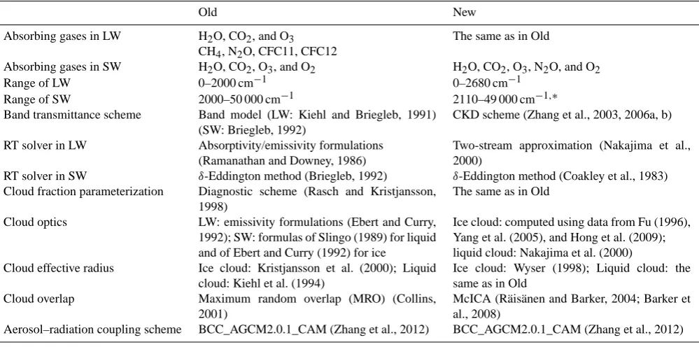
Fig. 3. The annual mean differences in SW CRF (left) and LW CRF (right). Differences larger (smaller) than 10 (−10) W m−2are shaded in yellow (blue). The global mean and root mean square values of each figure are also shown.
abundant high-level ice clouds exist in all the ITCZ regions. Differences in SW CRF over mid–high latitudes are much smaller. There are only minor differences in areas with large SW CRF along 60◦S, where a large number of low-level clouds (mostly liquid) exist, because the liquid cloud optics in the two configurations are almost equivalent for CRF cal-culation. Consequently, the changes in ice cloud optical prop-erties are the main cause of the changes in SW in the run with the new configuration when maximum-random overlap of plane-parallel horizontally homogeneous clouds is assumed. In the OLD run, LW CRF is overestimated over most of the tropical and subtropical oceans with very few exceptions, but it is underestimated over intensively convective tropical regions such as the central Africa, the west Pacific warm pool, and the Amazon forests of South America (Fig. 3b). The N_MRO run produces similar distributions of these bi-ases; however, the positive biases in the tropical and sub-tropical oceans are reduced, whereas the negative biases are enhanced somewhat (Fig. 3d). The differences in LW CRF between the new and old configurations (see Fig. 3f) show a quite similar geographic distribution to those of SW CRF (see Fig. 3e), with a maximum value of more than−9 W m−2
in the tropical east Pacific. Again, variations in ice cloud op-tics play a critical role in causing these differences.
Fig. 4. Zonal annual mean clear-sky and all-sky LW heating rates for OLD (a, d), N_MRO (b, e) and the differences between N_MRO and
OLD (c, f) (units: K day−1).
Table 2. The modeled and observed (SW CRF / LW CRF) ratios in
the tropical warm pool region (10◦S–20◦N, 110–160◦E).
OLD N_MRO OBS
ANN −1.17 −0.94 −1.13 DJF −1.55 −1.34 −1.14 JJA −1.83 −1.51 −1.09
Radiative heating/cooling within the atmosphere is a crit-ical driving factor in climate simulations. Figure 4 compares the clear-sky and all-sky LW heating rates (HRs) of N_MRO and OLD, respectively. The differences in SW HR are much smaller than those in LW HR (figure not shown). For the clear-sky condition, N_MRO shows a remarkable (more than 10 %) increased radiative cooling in the lower troposphere within 60◦S–60◦N and a reduced radiative cooling in most of the middle troposphere. These may be related to the differ-ent treatmdiffer-ents of greenhouse gases, especially O3and water vapor. The difference in the all-sky LW HR (see Fig. 4f) is similar to the pattern shown in Fig. 4c, indicating that the dif-ferences in the HR of clouds are less important for determin-ing the all-sky HR differences in this case. This pattern tends to increase the stability of the atmosphere below 600 hPa but enhance vertical mixing above 600 hPa.
As shown above, the application of the BCC-RAD radia-tion scheme, without tuning the subgrid cloud structures, re-markably influences the radiation budget at both boundaries and within the atmosphere. These changes will extensively affect the final simulated climate.
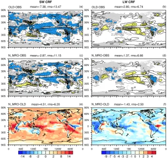
Fig. 5. Zonal annual mean (a) surface temperature and (c)
precipi-tation from N_MRO, OLD, and observation data, as well as (b, d) the differences between N_MRO and observations (red solid lines) and between OLD and observations (blue solid lines). The observa-tion data for temperature are from the ERA-Interim reanalysis, and those for precipitation are from the Xie and Arkin (1997) data set.
4.1.2 Surface climatology
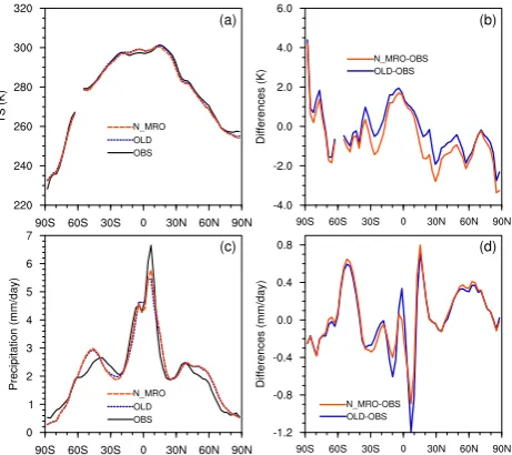
Fig. 6. Biases in zonal annual mean atmospheric temperature and specific humidity compared with the ERA-Interim reanalysis for (a, d)
OLD and (b, e) N_MRO simulations and (c, f) the differences between N_MRO and OLD.
Zonal comparisons of surface temperature (ST, for land only) and precipitation rate are shown in Fig. 5. There are substantial differences between the simulations and the ERA-Interim reanalysis (Uppala et al., 2005), which is av-eraged over the same period as the simulations. For in-stance, simulated STs are underestimated by about 1.5 K in the mid-latitudes and by about 3 K around the North Pole (see Fig. 5b), but overestimated by about 2 K and 4 K over the tropics and South Pole, respectively. The global distribu-tions of surface temperature biases for the N_MRO and OLD runs are quite similar (figures not shown), with local maxi-mum differences between the N_MRO and OLD runs reach-ing±2–4 K. The differences between the simulations and ob-servations are much larger than the differences between the N_MRO and OLD simulations. It should be noted that the SSTs used here are prescribed, which limited the model re-sponse.
Similar to Fig. 5a and b, Fig. 5c and d show comparisons of the precipitation rate. Both the N_MRO and OLD simula-tions capture the main features of the meridional distribution of precipitation, such as the maximum in the tropics and sec-ondary maxima at the mid-latitude storm tracks. However, er-rors are also clear relative to the observation, especially in the tropics. The two simulations are comparable in the simula-tion of the zonal mean distribusimula-tion of precipitasimula-tion, but there are noticeable local differences in the tropical and subtropical regions (figures not shown). These differences probably stem
from the altered atmospheric thermodynamics and dynamics caused by the changes in radiation budget. The increases and decreases in precipitation often coincide with the decreases and increases in surface temperature (figures not shown), re-spectively; thus, the changes in precipitation also obviously influence the surface energy balance.
4.1.3 Atmospheric states
Simulated atmospheric temperature and specific humidity are analyzed in this subsection.
Figure 6 shows the comparisons of the latitude–height dis-tribution of atmospheric temperature and specific humidity. Notable cold biases relative to ERA-Interim, about 1–2 K in the low–mid troposphere, exist throughout almost the en-tire troposphere in the OLD case (see Fig. 6a). The N_MRO simulation inherits most of these biases, but the relative warming (up to 0.4–0.8 K) within the middle troposphere (800∼500 hPa) is a desirable change compared with OLD (see Fig. 6c). This is definitely related to the reduced LW cooling rate in the middle troposphere, as shown in Fig. 4.
the N_MRO run notably increases the specific humidity in the tropics, typically reducing the original biases by about 30 %.
The changes in atmospheric temperature and specific hu-midity exert influences on the formation and maintenance of cloud water and ice (figures not shown), affecting the modeled local radiation budget, such as altering the (SW CRF) / (LW CRF) ratio mentioned above.
Overall, the incorporation of the new scheme influences radiative fluxes and heating rates remarkably. Due to these changes, the simulated surface and atmospheric climate are comparable or improved relative to the old model configura-tion. Therefore, the new scheme used here has been demon-strated to be a viable option for long-term climate simulation. It should also be mentioned that the differences in simu-lated climate between the two model configurations are rela-tively smaller than those between the simulations and obser-vations. Nevertheless, the much more flexible cloud structure and internal consistency of the new configuration will benefit further development of model physics. In regard to the conve-nience of the McICA scheme for modifying subgrid clouds, the impacts of the cloud structure variations are assessed as follows.
4.2 The impacts of altering subgrid cloud structures
In this subsection, we discuss the impacts of altering overlap-ping scheme of fractional clouds and breaking the traditional PPH assumption on simulated radiation and climate.
4.2.1 The impact of altering cloud overlap
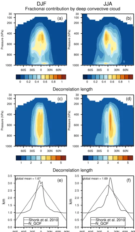
In Fig. 7, the top panels show the zonal mean distributions of the fractional contribution by deep convective cloud to total cloud (fcon/ftot)in GCM grid cells.fcon/ftothas the maxi-mum value in the upper tropics, then decreases sharply with latitude. There is a seasonal variation as shown in DJF and JJA. In the second row of Fig. 7, the latitude–height distribu-tions of the grid-cell meanLcfcalculated using Eq. (8) are shown. In general,Lcfreaches its maximum value in upper tropics, and decreases with latitude, similar to the distribu-tion offcon/ftot. That the decorrelation length tends to in-crease upwards has also been alluded by Barker (2008) and Räisänen et al. (2004).
In the bottom panels of Fig. 7, the zonal mean vertically averagedLcf(solid lines) is shown. Also shown is the Shonk et al. (2010) function result based merely on latitude (dashed lines). It is found thatLcf not only depends on geographi-cal location but also has seasonal variation as indicated in DJF and JJA. Therefore, it is difficult to parameterizeLcf only based on latitude. Though the scheme of N_GOF is not directly from observations, the result shown is very close to that derived from CloudSat/CALIPSO observations (see Fig. 1 in Oreopoulos et al., 2012). Through comparison with
Fig. 7. Zonal annual mean (a, b) fractional contribution by deep
convective cloud fraction (fcon/ftot)and (c, d)Lcfcalculated using
Eq. (8) from the N_GOF run, as well as (e, f) the vertically averaged
Lcffor N_GOF (solid lines) and that used by Shonk et al. (2010)
(dashed lines), for DJF (left) and JJA (right).
the standard scheme of N_GO2, the impact of cloud-type-relatedLcfcan be explored.
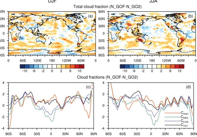
Fig. 8. Differences in (a, b) total cloud fraction between N_GOF and N_GO2, and (c, d) zonal mean differences in total (CTOT), low (CLOW),
middle (CMED), and high (CHGH)cloud fractions between N_GOF and N_GO2, for DJF (left) and JJA (right).
high clouds are presented separately. For the low and mid-dle clouds, it is found that the cloud fraction generally de-creases in the tropics and inde-creases in the middle and high lat-itudes, which is consistent with the total cloud fraction. How-ever, for high clouds, N_GOF generally produces a larger cloud fraction compared to N_GO2 even in the tropics. As the cloud fractions in individual layers do not change no-tably, the increased high cloud fraction is mostly because the decorrelation length in the upper troposphere is smaller in N_GOF than in N_GO2. Fewer low/middle clouds in the tropics causes more solar radiation to reach the lower atmo-sphere and surface, because high clouds have smaller impact on solar radiation compared to the low/middle clouds. The extra solar heating in the lower atmosphere and surface can enhance the surface evaporation and atmospheric convec-tion, which then can produce more cirrus clouds (Emmanuel, 1994).
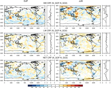
In the top panels of Fig. 9, the differences in SW CRF between N_GOF and N_GO2 are shown. The differences in SW CRF can exceed 15 W m−2 over a large domain in the tropical regions. In the regions with more convective clouds (for instance, the summer northern Indian Ocean and tropical Atlantic Ocean), the larger chance of maximum overlap leads to less cloud solar reflection, and thereby less SW CRF (pos-itive differences between N_GOF and N_GO2). Similarly, in the regions with fewer convective clouds (for instance, the summer Arctic and winter Southern Hemisphere oceans), the difference between the two schemes becomes negative. The zonal mean results show that SW CRF generally increases in the tropics and decreases in the middle and high latitudes.
The middle panels of Fig. 9 show the differences in LW CRF between N_GOF and N_GO2. In the regions with more convective clouds, the smaller cloud fraction shades less longwave radiation from reaching outer space, thereby caus-ing less LW CRF. Similarly, in the regions of fewer convec-tive clouds, LW CRF is increased. The zonal mean results show that the LW CRF is generally increased by N_GOF in the middle and high latitudes. However the change in the tropics is small. LW CRF is strongly dependent on high clouds. As shown in Fig. 8, the change in high cloud fraction in the tropics is different from that in low/middle clouds.
The changes of SW and LW CRFs are generally opposite. For example, over the summer northern Indian Ocean and tropical Atlantic Ocean, a positive SW CRF difference corre-sponds to a negative LW CRF difference. However, the solar effect is generally stronger than that of longwave. The net ef-fect in the total CRF does not cancel out. In the lower panels of Fig. 9, the differences in total CRF are shown. From the zonal mean result, a more strongly positive CRF in the sum-mer Arctic is clearly seen. Despite the obvious differences of CRFs at the TOA in different latitudes, the global mean dif-ferences in net fluxes are small (Fig. 1b, h) at the TOA, due to compensation between latitudes.
Fig. 9. Differences in (a, b) SW CRF, (c, d) LW CRF, (e, f) net CRF at the TOA between N_GOF and N_GO2, for DJF (left) and JJA (right).
that it can respond to climate change (i.e., if the distribu-tion of convective cloud changes in a climate change exper-iment, so will the decorrelation length). This is not the case for the latitude-dependent and Julian-day-dependent decor-relation parameterizations of Shonk and Hogan (2010) and Oreopoulos et al. (2012).
In Fig. 10, the top panels show the change in net radiative flux at the TOA, which is equivalent to the change in energy balance at the TOA. It is found that the energy balance at the TOA has been considerably affected by addressing the cloud-type-relatedLcf. N_GOF leads to an obvious increase of net flux in the tropics (especially for the JJA season) and high-latitude regions. In the subtropical high-pressure regions, the change in net flux is relatively small because the cloud frac-tion is low there. The change in energy balance from the trop-ics to the subtropical high regions can influence Hadley cir-culation. The same as the result at TOA, the largest changes in surface energy balance occur in the tropics and high lati-tudes. It is worth emphasizing that the change in energy bal-ance in Arctic is large, which should have very strong impact on the evolution of sea ice. Investigating the impact on polar climate by N_GOF will be a subsequent work for us.
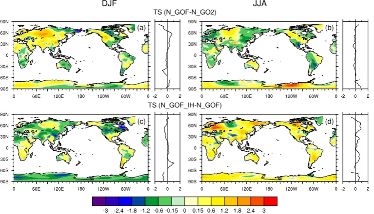
Figure 11a and b are the land surface temperature differ-ences between N_GOF and N_GO2. The patterns are simi-lar to those of the differences in net CRF at the surface as
shown in Fig. 10c and d over land. For DJF, most land sur-faces are simulated warmer by N_GOF than by N_GO2, as net CRF over these areas is more positive for N_GOF. The JJA season sees more negative differences between N_GOF and N_GO2. The range of differences is generally between −3 and 3 K.
4.2.2 The impact of breaking the PPH assumption
In this subsection, we briefly consider the impact of break-ing the traditional PPH assumption on the simulated radia-tion and climate by comparing the N_GOF_IH and N_GOF tests, where N_GOF_IH employs the same vertical overlap scheme as N_GOF but with consideration of the horizontal inhomogeneity in cloud condensate as discussed in Sect. 3.
Fig. 10. Differences in net radiative budget (a, b) at the TOA and (c, d) at the surface between N_GOF and N_GO2, for DJF (left) and JJA
(right).
Fig. 11. Differences in simulated surface temperature (a, b) between N_GOF and N_GO2 and (c, d) between N_GOF_IH and N_GOF, for
DJF (left) and JJA (right).
ECHAM5 data set. Both of these two are offline calculations; thus no climate interactions are included. The consideration of horizontally inhomogeneous clouds here brings the global mean CRFs andFnetmuch closer to observations. In general, N_GOF_IH is the best among all the simulations in terms of the global mean radiative fluxes. However, the spatial distri-butions of CRF biases of N_GOF_IH are similar to those of other simulations (see Fig. 12), which requires revision of
not only the radiation scheme but also the other parts of the model.
Fig. 12. The same as Fig. 3 (c, d), but for the simulation N_GOF_IH.
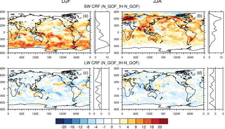
Fig. 13. Differences in (a, b) SW CRF and (c, d) LW CRF between N_GOF_IH and N_GOF, for DJF (left) and JJA (right).
cloud condensate generally overestimates solar reflectance (Carlin et al., 2002). The zonal mean results show that en-hancements of SW CRF mostly happen in high latitudes for both the boreal summer and austral summer. Barker and Räisänen (2005) got very similar zonal distribution of SW sensitivity to cloud inhomogeneity by computing on a CSRM data set, with zonal maximum of as large as ∼25 W m−2 around 60◦S.
The inclusion of horizontal inhomogeneity of cloud con-densate generally reduces LW CRF all over the globe (Fig. 13c, d). This is because the PPH assumption of cloud condensate generally overestimates the LW emissivity up-wards (Pomroy and Illingworth, 2000). The patterns of change in SW and LW CRFs are very similar. However, the zonal mean results of LW CRF do not show very special fea-tures in the boreal or austral summer. This is also similar to results of Barker and Räisänen (2005). LW CRF shows less dependence on season probably because LW CRF does not increase proportionally with the incoming solar flux at the TOA.
The magnitude of the local change of CRFs by address-ing cloud inhomogeneity is about the same as changaddress-ingLcf (compared with Fig. 10). Thus, it is of great importance to address the cloud water/ice horizontal distribution together with the overlap of fractional clouds in GCMs.
The consideration of cloud horizontal inhomogeneity has a noticeable influence on surface temperature (see Fig. 11c, d). In the middle and high latitudes of the Northern Hemisphere, there is a remarkable decrease in surface temperature during DJF and an increase during JJA. These changes arise mainly from competition between LW cooling and SW heating. When inhomogeneous clouds succeed homogeneous ones, more LW flux is emitted outward, and more SW flux pen-etrates to the surface (see Fig. 1). The surface energy budget is then the net effect of the two fluxes.
model configuration can be used in BCC_AGCM2.0.1 to im-prove physical processes and perform climate simulations.
It should be noted that, in this work, we altered only the subgrid cloud structures used in the radiation calcula-tion, whereas those in precipitation parameterization were not changed. Physically, cloud overlap assumptions in the ra-diation and precipitation processes should be consistent with each other, but the latter may have a larger effect on the sim-ulated precipitation (Morcrette and Jakob, 2000). However, this is beyond the scope of this study.
5 Discussion and conclusions
In this work, the BCC-RAD radiation algorithm was incorpo-rated into the BCC_AGCM2.0.1 GCM as a replacement for the original radiation algorithm. The new radiation is entirely distinct from the original one, by including the advanced treatments of gaseous absorption, cloud optics and radiation transfer. The results show that the new scheme markedly im-proves the representation of the SW and LW radiation bud-get for both clear-sky and all-sky conditions, whether in the global mean or in geographic distribution. The simulated lationship between SW and LW CRFs in deep convective re-gions is improved by the new scheme as well. The modeled temperature and specific humidity benefited from changes in the LW heating rate, resulting in a reduction in temperature biases by 0.4–0.8 K at the middle troposphere and a reduc-tion in moisture biases by one-third in the tropical lower tro-posphere relative to the ERA-Interim reanalysis. This shows the superiority of a CKD radiation algorithm to the band-model-based CAM3 radiation scheme. All these results in-dicate that using the BCC-RAD radiation scheme makes the cloud-radiation process more intrinsically coherent and rea-sonable.
The McICA scheme was applied to the BCC-RAD radi-ation algorithm to deal with cloud subgrid variability. This new configuration is flexible for treating arbitrarily com-plex subgrid cloud structures, including the vertical overlap of fractional clouds and the horizontal distribution of cloud condensate. The impact of altering cloud overlap within the McICA scheme was assessed by including a so-called “gen-eral overlap” with a global constantLcfof 2 km. In this work we have also considered a cloud-type-relatedLcf, which es-pecially distinguishes the deep convective cloud from other types of clouds. This scheme yields a similar zonal mean dis-tribution ofLcf compared to the CloudSat/CALIPSO result demonstrated by Oreopoulos et al. (2012). One advantage of the cloud-dependent decorrelation length described in this ar-ticle is that it can respond to climate change. The new cloud-type-relatedLcfhas remarkable effect on local radiation bud-get compared to the scheme of constantLcf. In the regions of frequent convection such as South Asia monsoon region and ITCZ, CRF is most notably influenced, with local differences of > 20 W m−2for SW CRF and > 10 W m−2 for LW CRF.
Generally, more net energy reaches surface around the trop-ics while less reaches the surface in mid–high latitudes. This could enhance the simulated Hadley circulation. Therefore, a constant value ofLcfcould lead to large biases in climate simulations.
The effect of the horizontal inhomogeneity of cloud con-densate was then considered by including an observation-based gamma function in an additional test. The changes compared with its PPH counterpart were strikingly signifi-cant, with decreases in the global mean TOA LW and SW CRFs of∼1.5 W m−2and∼3.7 W m−2, respectively, mak-ing the simulation much closer to observations. This empha-sizes the importance of addressing the cloud horizontal dis-tribution in GCMs along with the cloud overlap issue.
For simulated climate, the changes in cloud structures showed a notable effect on surface temperatures in mid–high latitudes, with the largest zonal mean differences being about 1 K, exceeding the differences between the new and old radi-ation scheme configurradi-ations when both use the maximum-random overlap and PPH assumptions. This will exert an effect on the evolution of sea ice. In this work, we did not include sea–atmosphere interaction, which could enlarge the effect of the signal imposed by the changing cloud structures. This study shows that N_GOF_IH is the current best choice for climate simulations, and it will be adopted in BCC_AGCM2.0.1.
This study also provided a direction for future improve-ment of the McICA. More realistic cloud overlap assump-tion or cloud horizontal distribuassump-tion, achieved from satellite observations or any other objective sources, could be used to constrain the generation of cloud-type-relatedLcfand the horizontal distribution of cloud condensate.
Acknowledgements. This work was financially
sup-ported by National Basic Research Program of China (2011CB403405 & 2012CB955303), the National Natural Science Foundation of China (grant nos. 41075056) and Public Meteo-rology Special Foundation of MOST (GYHY201406023). The authors would like to thank Howard W. Barker and Jason N. Cole for providing the McICA and SCG codes, and thank the two anony-mous reviewers for their helpful and constructive suggestions.
Edited by: W. Hazeleger
References
Barker, H. W.: Overlap of fractional cloud for radiation calculations in GCMs: A global analysis using CloudSat and CALIPSO data. J. Geophys. Res., 113, D00A01, doi:10.1029/2007JD009677, 2008.
Barker, H. W. and Räisänen, P.: Radiative sensitivities for cloud structural properties that are unresolved by conventional GCMs, Q. J. Roy. Meteorol. Soc., 131, 3103–3122, 2005.
independent column approximation: an assessment using sev-eral global atmospheric models, Q. J. Roy. Meteorol. Soc., 134, 1463–1478, 2008.
Baum, B. A., Heymsfield, A. J., Yang, P., and Bedka, S. T.: Bulk Scattering Properties for the Remote Sensing of Ice Clouds. Part I: Microphysical Data and Models, J. Appl. Meteorol., 44, 1885– 1895, 2005.
Baum, B. A., Yang, P., Heymsfield, A. J., Schmitt, C., Xie, Y., Bansemer, A., Hu, Y. X., and Zhang, Z.: Improvements to short-wave bulk scattering and absorption models for the remote sens-ing of ice clouds, J. Appl. Meteorol. Clim., 50, 1037–1056, 2011. Briegleb, B. P.: Delta-Eddington approximation for solar radiation in the NCAR Community Climate Model, J. Geophys. Res., 97, 7603–7612, 1992.
Carlin, B., Fu, Q., Lohmann, U., Mace, G. G., Sassen, K., and Com-stock, J. M.: High-Cloud Horizontal Inhomogeneity and Solar Albedo Bias, J. Climate, 15, 2321–2339, 2002.
Clough, S. A. and Iacono, M. J.: Line-by-line calculation of atmo-spheric fluxes and cooling rates 2: Application to carbon dioxide, ozone, methane, nitrous oxide and the halocarbons, J. Geophys. Res., 100, 16519–16535, 1995.
Coakley, J. A., Cess, R. D., and Yurevich, F. B.: The Effect of Tro-pospheric Aerosols on the Earth’sRadiation Budget: A Parame-terization for Climate Models, J. Atmos. Sci., 40, 116–138, 1983. Collins, W. D.: Parameterization of Generalized Cloud Overlap for Radiative Calculations in General Circulation Models, J. Atmos. Sci., 58, 3224–3242, 2001.
Collins, W. D., Hackney, J. K., and Edwards, D. P.: An updated parameterization for infrared emission and absorption by wa-ter vapor in the National Cenwa-ter for Atmospheric Research Community Atmosphere Model, J. Geophys. Res., 107, 4664, doi:10.1029/2001JD001365, 2002.
Ebert, E. E. and Curry, J. A.: A Parameterization of Ice Cloud Op-tical Properties for Climate Models, J. Geophys. Res., 97, 3831– 3836, 1992.
Ellingson, R. G., Ellis, J., and Fels, S.: The Intercomparison of Ra-diation Codes Used in Climate Models: Long Wave Results, J. Geophys. Res., 96, 8929–8953, 1991.
Emmanuel, K. A.: Atmospheric Convection, Oxford: Oxford Uni-versity Press, 580 pp., 1994.
Fu, Q.: An Accurate Parameterization of the solar radiative prop-erties of cirrus clouds for climate models, J. Climate, 9, 2058– 2082, 1996.
Fu, Q. and Liou, K. N.: On the Correlatedk-Distribution Method for Radiative Transfer in Nonhomogenecous Atmospheres, J. At-mos. Sci., 49, 2139–2156, 1992.
Gong, S. L., Barrie, L. A., Blanchet, J. P., von Salzen, K., Lohmann, U., Lesins, G., Spacek, L., Zhang, L. M., Girard, E., Lin, H., Leaitch, R., Leighton, H., Chylek, P., and Huang, P.: Canadian Aerosol Module: A size-segregated simulation of atmospheric aerosol processes for climate and air quality models 1. Module development, J. Geophys. Res., 108, 4007, doi:10.1029/2001JD002002, 2003.
Hill, P. G., Manners, J., and Petch, J. C.: Reducing noise associated with the Monte Carlo Independent Column Approximation for weather forecasting models, Q. J. Roy. Meteorol. Soc., 137, 219– 228, 2011.
Hogan, R. J. and Illingworth, A. J.: Deriving cloud overlap statistics from radar, Q. J. Roy. Meteorol. Soc., 128, 2903–2909, 2000.
Hong, G., Yang, P., Baum, B. A., Heymsfield, A. J., and Xu, K. M.: Parameterization of Shortwave and Longwave Radiative Prop-erties of Ice Clouds for Use in Climate Models, J. Climate, 22, 6287–6312, 2009.
Kiehl, J. T. and Briegleb, B. P.: A new parameterization of the ab-sorptance due to the 15 µm band system of carbon dioxide, J. Geophys. Res., 96, 9013–9019, 1991.
Kiehl, J. T. and Ramanathan, V.: Comparison of Cloud Forcing De-rived From the Earth Radiation Budget Experiment with That Simulated by the NCAR Community Climate Model, J. Geo-phys. Res., 95, 11679–11698, 1990.
Kiehl, J. T., Hack, J. J., and Briegleb, B. P.: The simulated Earth ra-diation budget of the National Center for Atmospheric Research Community Climate Model CCM2 and comparisons with the Earth Radiation Budget Experiment (ERBE), J. Geophys. Res., 99, 20815–20827, 1994.
Kratz, D. P.: The correlatedk-distribution technique as applied to the AVHRR channels, J. Quant. Spectrosc. Ra., 53, 501–517, 1995.
Kristjansson, J. E., Edwards, J. M., and MitChell, D. L.: Impact of a new scheme for optical properties of ice crystals on climates of two GCMs, J. Geophys. Res., 105, 10063–10079, 2000. Li, J. and Barker, H. W.: A Radiation Algorithm with Correlated-k
Distribution. Part I: Local Thermal Equilibrium, J. Atmos. Sci., 62, 286–309, 2005.
Loeb, N. G., Wielicki, B. A., Doelling, D. R., Smith, G. L., Keyes, D. F., Kato, S., Manalo-Smith, N., and Wong, T.: Toward opti-mal closure of the Earth’s top-of-atmosphere radiation budget, J. Climate, 22, 748–766, 2009.
Lu, P., Zhang, H., and Jing, X. W.: The effects of different HITRAN versions on calculated long-wave radiation and uncertainty eval-uation, Acta Meteorol. Sin., 26, 389–398, 2012.
Mace, G. G. and Benson-Troth, S.: Cloud-Layer Overlap Charac-teristics Derived from Long-Term Cloud Radar Data, J. Climate, 15, 2505–2515, 2002.
Mishchenko, M. I., Travis, L. D., and Lacis, A. A.: Scattering, Ab-sorption, and Emmision of Light by Small Particles, Cambridge University press, 2002.
Mlawer, E. J., Taubman, S. J., Brown, P. D., Iacono, M. J., and Clough, S. A.: Radiative transfer for inhomogeneous atmo-spheres: RRTM, a validated correlated-k model for the longwave, J. Geophys. Res., 102, 16663–16682, 1997.
Morcrette, J. J. and Jakob, C.: The Response of the ECMWF Model to Changes in the Cloud Overlap Assumption, Mon. Weather Rev., 128, 1707–1732, 2000.
Morcrette, J. J., Barker, H. W., Cole, J. S., Iacono, M. J., and Pincus, R.: Impact of a new radiation package, McRad, in the ECMWF Integrated Forecasting System, Mon. Weather Rev., 136, 4773– 4798, doi:10.1175/2008MWR2363.1, 2008.
Nakajima, T., Tsukamoto, M., Tsushima, Y., Numaguti, A., and Kimura, T.: Modeling of the Radiative Process in an Atmospheric General Circulation Model, Appl. Optics, 39, 4869–4878, 2000. Naud, C. M., Del Genio, A., Mace, G. G., Benson, S., Clothiaux, E. E., and Kollias, P.: Impact of Dynamics and Atmospheric State on Cloud Vertical Overlap, J. Climate, 21, 1758–1770, 2008. Neale, R. B., Chen, C. C., Andrew, G., Lauritzen, P. H., Park,
Collins, W. D., Iacono, M. J., Easter, R. C., Ghan, S. J., Liu, X., Rasch, P. J., and Taylor, M. A.: Description of the NCAR Community Atmosphere Model (CAM 5.0). NCAR Tech. Note TN-486, available at: http://www.cesm.ucar.edu/ models/cesm1.2/cam/docs/description/cam5_desc.pdf (last ac-cess: 30 April 2014), 2010.
Neggers, R. A. J., Heus, T., and Siebesma, A. P.: Over-lap statistics of cumuliform boundary-layer cloud fields in large-eddy simulations, J. Geophys. Res., 116, D21202, doi:10.1029/2011JD015650, 2011.
Oleson, K. W., Bonan, G. B., Schaaf, C., Gao, F., Jin, Y., and Strahler, A.: Assessment of global climate model land sur-face albedo using MODIS data, Geophys. Res. Lett., 30, 1443, doi:10.1029/2002GL016749, 2003.
Oreopoulos, L., Lee, D., Sud, Y. C., and Suarez, M. J.: Radiative im-pacts of cloud heterogeneity and overlap in an atmospheric Gen-eral Circulation Model, Atmos. Chem. Phys., 12, 9097–9111, doi:10.5194/acp-12-9097-2012, 2012.
Pincus, R., Barker, H. W., and Morcrette, J. J.: A fast, flex-ible, approximate technique for computing radiative transfer in inhomogeneous cloud fields, J. Geophys. Res., 108, 4376, doi:10.1029/2002JD003322, 2003.
Pomroy, H. R. and Illingworth, A. J.: Ice cloud inhomogeneity: Quantifying bias in emissivity from radar observations, Geophys. Res. Lett., 27, 2101–2104, 2000.
Räisänen, P. and Barker, H. W.: Evaluation and optimization of sam-pling errors for the Monte Carlo Independent Column Approxi-mation, Q. J. Roy. Meteorol. Soc., 130, 2069–2085, 2004. Räisänen, P. and Järvinen, H.: Impact of cloud and radiation scheme
modifications on climate simulated by the ECHAM5 atmo-spheric GCM, Q. J. Roy. Meteorol. Soc., 136, 1733–1752, 2010. Räisänen, P., Barker, H. W., Khairoutdinov, M. F., Li, J., and Randall, D. A.: Stochastic generation of subgrid-scale cloudy columns for large-scale models, Q. J. Roy. Meteorol. Soc., 130, 2047–2067, 2004.
Räisänen, P., Järvenoja, S., Järvinen, H., Giorgetta, M., Roeckner, E., Jylhä, K., and Ruosteenoja, K.: Tests of Monte Carlo Inde-pendent Column Approximation in the ECHAM5 Atmospheric GCM, J. Climate, 20, 4995–5011, 2007.
Ramanathan, V. and Downey, P.: A nonisothermal emissivity and absorptivity formulation for water vapor, J. Geophys. Res., 91, 8649–8666, 1986.
Randles, C. A., Kinne, S., Myhre, G., Schulz, M., Stier, P., Fischer, J., Doppler, L., Highwood, E., Ryder, C., Harris, B., Huttunen, J., Ma, Y., Pinker, R. T., Mayer, B., Neubauer, D., Hitzenberger, R., Oreopoulos, L., Lee, D., Pitari, G., Di Genova, G., Quaas, J., Rose, F. G., Kato, S., Rumbold, S. T., Vardavas, I., Hatzianas-tassiou, N., Matsoukas, C., Yu, H., Zhang, F., Zhang, H., and Lu, P.: Intercomparison of shortwave radiative transfer schemes in global aerosol modeling: results from the AeroCom Radia-tive Transfer Experiment, Atmos. Chem. Phys., 13, 2347–2379, doi:10.5194/acp-13-2347-2013, 2013.
Rasch, P. J. and Kristjansson, J. E.: A comparison of the CCM3 model climate using diagnosed and predicted condensate param-eterizations, J. Climate, 11, 1587–1614, 1998.
Rayner, N. A., Parker, D. E., Horton, E. B., Folland, C. K., Alexan-der, L. V., Powell, D. P., Kent, E. C., and Kaplan, A.: Global analyses of sea surface temperature, sea ice, and night marine air
temperature since the late nineteenth century, J. Geophys. Res., 108, 4407, doi:10.1029/2002JD002670, 2003.
Reynolds, R. W., Rayner, N. A., Smith, T. M., Stokes, D. C., and Wang, W.: An improved in situ and satellite SST analysis for climate, J. Climate, 15, 1609–1625, 2002.
Rothman, L. S., Barbe, A., Chris Benner, D., Brown, L. R., Camy-Peyret, C., Carleer, M. R., Chance, K., Clerbaux, C., Dana, V., Devi, V. M., Fayt, A., Flaud, J. M., Gamache, R. R., Goldman, A., Jacquemart, D., Jucks, K. W., Lafferty, W. J., Mandin, J. Y., Massie, S. T., Nemtchinov, V., Newnham, D. A., Perrin, A., Rins-land, C. P., Schroeder, J., Smith, K. M., Smith, M. A. H., Tang, K., Toth, R. A., Vander Auwera, J., Varanasi, P., and Yoshino, K.: The HITRAN molecular spectroscopic database: edition of 2000 including updates through 2001, J. Quant. Spectrosc. Ra., 82, 5–44, 2003.
Shi, G.-Y., Xu, N., Wang, B., Dai, T., and Zhao, J.-Q.: An improved treatment of overlapping absorption bands based on the corre-latedkdistribution model for thermal infrared radiative transfer calculations, J. Quant. Spectrosc. Ra., 110, 435–451, 2009. Shonk, J. K. P. and Hogan, R. J.: Effect of improving representation
of horizontal and vertical cloud structure on the Earth’s global radiation budget. Part II: The global effects, Q. J. Roy. Meteorol. Soc., 136, 1205–1215, 2010.
Shonk, J. K. P., Hogan, R. J., Edwards, J. M., and Mace, G. G.: Ef-fect of improving representation of horizontal and vertical cloud structure on the Earth’s global radiation budget. Part I: Review and parametrization, Q. J. Roy. Meteorol. Soc., 136, 1191–1204, 2010.
Slingo, A.: A GCM Parameterization for the Shortwave Radiative Properties of Water Clouds, J. Atmos. Sci., 46, 1419–1427, 1989. Tian, L. and Curry, J. A.: Cloud Overlap Statistics, J. Geophys. Res.,
94, 9925–9935, 1989.
Uppala, S. M., KÅllberg, P. W., Simmons, A. J., Andrae, U., da Costa Bechtold, V., Fiorino, M., Gibson, J. K., Haseler, J., Her-nandez, A., Kelly, G. A., Li, X., Onogi, K., Saarinen, S., Sokka, N., Allan, R. P., Andersson, E., Arpe, K., Balmaseda, M. A., Beljaars, A. C. M., Van De Berg, L., Bidlot, J., Bormann, N., Caires, S., Chevallier, F., Dethof, A., Dragosavac, M., Fisher, M., Fuentes, M., Hagemann, S., Hólm, E., Hoskins, B. J., Isaksen, L., Janssen, P. A. E. M., Jenne, R., McNally, A. P., Mahfouf, J. F., Morcrette, J. J., Rayner, N. A., Saunders, R. W., Simon, P., Sterl, A., Trenberth, K. E., Untch, A., Vasiljevic, D., Viterbo, P., and Woollen, J.: The ERA-40 re-analysis, Q. J. Roy. Meteorol. Soc., 131, 2961–3012, 2005.
Wei, X. D. and Zhang, H.: Analysis of optical properties of nonspherical dust aerosols, Acta Optica. Sinica, 31, 0501002, doi:10.3788/aos201131.0501002, 2011.
Wu, T. W. and Wu, G. X.: An empirical formula to compute snow cover fraction in GCMs, Adv. Atmos. Sci., 21, 529–535, 2004. Wu, T., Yu, R., Zhang, F., Wang, Z., Dong, M., Wang, L., Jin,
X., Chen, D., and Li, L.: The Beijing Climate Center atmo-spheric general circulation model: description and its perfor-mance for the present-day climate, Clim. Dynam., 34, 123–147, doi:10.1007/s00382-008-0487-2, 2010.
Wyser, K.: The Effective Radius in Ice Clouds, J. Climate, 11, 1793–1802, 1998.
Numerical Model Outputs, B. Am. Meteorol. Soc., 78, 2539– 2558, 1997.
Yan, H.: The design of a nested fine-mesh model over complex to-pography part 2: parameterization of sub grid physical processes, Plateau Meteorol., 6, 64–139, 1987 (in Chinese).
Yang, P., Wei, H., Huang, H. L., Baum, B. A., Hu, Y. X., Kattawar, G. W., Mishchenko, M. I., and Fu, Q.: Scattering and absorp-tion property database for nonspherical ice particles in the near-through far-infrared spectral region, Appl. Optics., 44, 5512– 5523, 2005.
Yang, P., Bi, L., Baum, B. A., Liou, K. N., Kattawar, G. W., Mishchenko, M. I., and Cole, B.: Spectrally consistent scatter-ing, absorption, and polarization properties of atmospheric ice crystals at wavelengths from 02 to 100 µm, J. Atmos. Sci., 70, 330–347, 2013.
Zhang, F., Liang, X. Z., Li, J., and Zeng, Q.: Dominant roles of subgrid-scale cloud structures in model diversity of cloud radiative effect, J. Geophys. Res., 118, 7733–7749, doi:10.1002/jgrd.50604, 2013.
Zhang, G. and Mu, M.: Effects of modification to the Zhang-Mcfarlane convection parameterization on the simulation of the tropical precipitation in the National Center for Atmosphere Re-search Community Climate Model, Version 3, J. Geophys. Res., 110, D09109, doi:10.1029/2004JD005617, 2005.
Zhang, H., Nakajima, T., Shi, G., Suzuki, T., and Imasu, R.: An opti-mal approach to overlapping bands with correlatedk-distribution method and its application to radiative calculations, J. Geophys. Res., 108, 4641, doi:10.1029/2002JD003358, 2003.
Zhang, H., Shi, G., Nakajima, T., and Suzuki, T.: The effect of the choice of thek-interval number on radiative calculation, J. Quant. Spectrosc. Ra., 98, 31–43, 2006a.
Zhang, H., Suzuki, T., Nakajima, T., Shi, G., Zhang, X., and Liu, Y.: Effects of band division on radiative calculations, Opt. Eng., 45, 016002, doi:10.1117/1.2160521, 2006b.
Zhang, H., Wang, Z., Wang, Z., Liu, Q., Gong, S., Zhang, X., Shen, Z., Lu, P., Wei, X., Che, H., and Li, L.: Simulation of direct ra-diative forcing of aerosols and their effects on East Asian cli-mate using an interactive AGCM-aerosol coupled system, Clim. Dynam., 38, 1675–1693, 2012.