https://doi.org/10.5194/gmd-10-2547-2017 © Author(s) 2017. This work is distributed under the Creative Commons Attribution 3.0 License.
A multi-diagnostic approach to cloud evaluation
Keith D. Williams and Alejandro Bodas-Salcedo Met Office, FitzRoy Road, Exeter, EX1 3PB, UK
Correspondence to:Keith Williams ([email protected])
Received: 2 December 2016 – Discussion started: 3 January 2017
Revised: 26 April 2017 – Accepted: 27 April 2017 – Published: 6 July 2017
Abstract. Most studies evaluating cloud in general circula-tion models present new diagnostic techniques or observa-tional datasets, or apply a limited set of existing diagnostics to a number of models. In this study, we use a range of di-agnostic techniques and observational datasets to provide a thorough evaluation of cloud, such as might be carried out during a model development process. The methodology is illustrated by analysing two configurations of the Met Of-fice Unified Model – the currently operational configuration at the time of undertaking the study (Global Atmosphere 6, GA6), and the configuration which will underpin the United Kingdom’s Earth System Model for CMIP6 (Coupled Model Intercomparison Project 6; GA7).
By undertaking a more comprehensive analysis which in-cludes compositing techniques, comparing against a set of quite different observational instruments and evaluating the model across a range of timescales, the risks of drawing the wrong conclusions due to compensating model errors are minimized and a more accurate overall picture of model per-formance can be drawn.
Overall the two configurations analysed perform well, es-pecially in terms of cloud amount. GA6 has excessive thin cirrus which is removed in GA7. The primary remaining er-rors in both configurations are the in-cloud albedos which are too high in most Northern Hemisphere cloud types and sub-tropical stratocumulus, whilst the stratocumulus on the cold-air side of Southern Hemisphere cyclones has in-cloud albedos which are too low.
1 Introduction
The accurate simulation of cloud in general circulation models (GCMs) is of considerable importance across all timescales. At numerical weather prediction (NWP)
timescales of a few days or less, cloud amount as a forecast product is of direct relevance to a number of users (e.g. avia-tion, solar farms, etc.) and affects forecasts of other variables through its radiative impact on the surface temperature and the effects of diabatic heating on the large-scale circulation. On climate timescales, the radiative feedback from cloud on the global energy budget remains one of the largest uncer-tainties in determining the global climate sensitivity (Flato et al., 2013).
Traditionally, the evaluation of cloud has been limited to quantities which were perceived to be of interest to the end user, such as ground-based observations of total cloud amount (Mittermaier, 2012) or top-of-atmosphere (TOA) cloud radiative forcing (CRF; e.g. Gleckler et al., 2008). However, compensating errors within GCMs can result in a model performing well on such a limited set of metrics, de-spite the processes within the model being in error. A classic example is the simulation of subtropical stratocumulus, for which many GCMs simulate too little cloud cover, but the cloud which is simulated is too bright, the two errors com-pensating to result in a reasonable CRF (e.g. Williams et al., 2003; Nam et al., 2012).
Over recent years, a range of process-oriented diagnostic techniques have been developed which composite the data according to other large-scale variables, with the intention of reducing the chances of a model appearing to perform well due to compensating errors. Compositing variables have in-cluded the following, amongst others: large-scale vertical ve-locity, (Bony et al., 2004), various measures of lower tropo-spheric stability, (Klein and Hartmann, 1993; Williams et al., 2006; Myers and Norris, 2015), position relative to cyclone centre, (Klein and Jakob, 1999; Govekar et al., 2011) and cloud regime (Williams and Tselioudis, 2007).
evalua-tion. For example, the ‘total cloud amount’ obtained from ground-based ceilometers will be underestimated since they typically cannot detect the highest clouds. When these issues are known, they can be mitigated by sampling the model in a manner consistent with the observations (e.g. in this case, only considering model clouds up to the maximum height the ceilometer can detect). For cloud evaluation against satel-lite data, increasing use is being made of satelsatel-lite simulators which aim to emulate the observations by carrying out a con-sistent retrieval on the model. A number of satellite simula-tors have been brought together in the CFMIP (Cloud Feed-back Model Intercomparison Project) Observational Simula-tor Package (COSP; Bodas-Salcedo et al., 2011), which has now been included in many GCMs.
Arguably the best way to minimize issues around com-pensating model errors, observational error and model– observation comparison issues, is to routinely evaluate cloud in GCMs against a wide range of different observational datasets, using simulators where appropriate and using a range of diagnostic techniques in order to gain a consistent picture of model biases. In this study, we illustrate how the approach can be used for model development by applying a comprehensive cloud evaluation to two configurations of the Met Office Unified Model (UM).
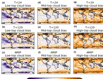
Cloud errors in the UM, possibly more than any other vari-able, are very similar across timescales and horizontal res-olutions (Williams and Brooks, 2008). Figure 1 shows the bias in high, middle and low cloud in the Global Atmo-sphere 6 (GA6; Walters et al., 2017a) configuration of the UM against CALIPSO (Cloud–Aerosol Lidar and Infrared Pathfinder Satellite Observation). It can be seen that the day 1 and day 5 forecast biases at N320 resolution (40 km in mid-latitudes) are very similar to each other and to a clima-tological bias obtained from an AMIP (Atmosphere Model Intercomparison Project; Gates, 1992) simulation at N96 res-olution (135 km in mid-latitudes). This means that we can make use of the strengths of each timescale in our anal-ysis, and the conclusions should be applicable across the systems. Although the UM is being used (a model which is routinely assessed for both NWP and climate work), we consider the cross-timescale approach a key aspect of the comprehensive evaluation. The initialized hindcasts provide case studies where model biases can be investigated in de-tail for particular meteorological events, in situations where the large-scale dynamics remain close to those observed. In contrast, the longer climate simulations provide charac-terization and statistics of the systematic errors. For those GCMs which are typically only used for a limited set of timescales, the AMIP (Gates, 1992) and Transpose-AMIP (Williams et al., 2013) experimental designs allow the possi-bility of this cross-timescale evaluation.
In the next section we provide details of the models, exper-iments and observational data subsequently presented. We then evaluate the cloud simulation in the model over the tropics, mid-latitude storm tracks and mid-latitude land in
Sects. 3, 4 and 5 respectively. The overall impact of the cloud on the global radiation balance is then discussed in Sect. 6. We summarize in Sect. 7.
2 Models and observational datasets 2.1 Models and experimental design
Two configurations of the UM are used in this study. GA6 has been operational in all global model systems at the Met Office since 15 July 2014 and is fully documented by Wal-ters et al. (2017a). GA7 has recently been frozen and is documented by Walters et al. (2017b). It is intended that GA7 will form the physical atmosphere model used by the United Kingdom Earth System Model 1 (UKESM1) which will be submitted to CMIP6 (Coupled Model Intercompari-son Project 6).
There are numerous physical parametrization changes be-tween GA6 and GA7 which are detailed in Walters et al. (2017b). Those of most relevance for this study are as fol-lows:
1. The introduction of a scheme to allow the turbulent fluxes within the boundary-layer capping inversion to be resolved and for clouds (“forced cumulus”) to form within it. The height of the top of the capping inver-sion is diagnosed using an energetic argument based on Beare (2008) which is applied to the calculation of an ascending air parcel used for the diagnosing convec-tion. Within the undulations of the capping inversion, if the parcel does not reach its level of free convection then forced cumulus may form. The cloud-base cloud fraction is parametrized as varying linearly with cloud depth, between a minimum of 0.1 and a maximum of 0.3 for cloud depths between 100 and 300 m, based loosely on the observations of (Zhang and Klein, 2013). Incre-ments to the overall prognostic cloud fraction are calcu-lated as necessary to increase it to the forced convective cloud fraction. The in-cloud water content is taken from the adiabatic parcel ascent in the cumulus diagnosis. 2. A package of changes designed to improve warm rain
de-(a)
(b)
(c)
(d)
(e)
(f)
(g)
(h)
(i)
Figure 1.Absolute bias (model field minus observed field) in GA6 configuration of the UM for low(a–c), mid-(d–f)and high(g–i)fractional cloud cover against the GCM-oriented CALIPSO cloud product (GOCCP), using the CALIPSO simulator in COSP (see Sect. 2.2). Panels (a),(d),(g)and(b),(e),(h)show mean biases at day 1 and day 5 averaged across all the NWP hindcasts at N320 (40 km in mid-latitudes) resolution. Panels(c),(f),(i)show the bias in the AMIP climatology at N96 (135 km in mid-latitudes) resolution.
rived from aircraft, CloudSat (Stephens et al., 2002) and CloudNet-ARM (Atmosphere Radiation Measurement) site observations.
3. Improved cloud ice optical properties and ice particle size distributions (PSDs) following Baran et al. (2014) and Field et al. (2007) respectively. The new PSD is an empirical fit that is better supported by observations and in GA7 is used consistently between the microphysics and radiation schemes.
4. Reduced rate of cirrus spreading by 2 orders of magni-tude. The cirrus spreading was a simple parametriza-tion intended to account for the spreading of cirrus through shear as it falls. It uses the model wind shear between successive layers to spread the ice as it falls, at a rate controlled by a tunable parameter. It was in-cluded, largely as a tuning of outgoing longwave radi-ation (OLR), in an earlier configurradi-ation (GA4; Walters et al., 2014) and it is desirable to reduce the effect until the scheme is developed on firmer physical grounds. 5. Addition of the turbulent production of liquid water in
mixed-phase clouds following Field et al. (2014). An exactly soluble stochastic model is used to describe sub-grid relative humidity fluctuations. The probability density function (PDF) of the fluctuations in a model grid box depends on the turbulent local state based on
the boundary-layer turbulent kinetic energy and on any pre-existing ice cloud. Increments to liquid water cloud prognostic fields are diagnosed from the PDF. This in-creases the liquid water contents and volume fractions of liquid cloud. A temperature threshold restricts the scheme to regions below 0◦C.
7. Although only small changes have been made to the scientific basis of the convection scheme, the numerics of the scheme have been re-written (the so-called “6A convection scheme”). This is described in Walters et al. (2017b), but the key points are as follows:
– Three iterations rather than one iteration are used to solve the implicit equations for the potential temperature of the detrained mass and the residual plume in the calculation of the forced detrainment. – Three rather than two iterations are used in deter-mining the potential temperature at saturation af-ter lifting the parcel from one level to the next un-der dry ascent. The evaporation of parcel conden-sate is now also allowed if the parcel becomes sub-saturated after entrainment and the dry ascent. – The ascent in the 6A scheme will terminate when
the mass flux falls below 5 % of its value at cloud base, which replaces the previous arbitrary small value.
– The convection scheme will introduce small errors in the conservation of energy and water. These are now corrected locally to ensure that the column in-tegral of these quantities is the same after the call to convection as they were before, replacing the pre-vious global correction.
For each configuration, two types of experiment have been conducted, both being standard tests used within the model development cycle for proposed changes to the UM. These are a 20-year (1988–2007) AMIP experiment run at a horizontal resolution of N96 (135 km in mid-latitude) and a set of 24 independent 5-day NWP hindcasts spread between December 2010 and August 2012, run at N320 (40 km in mid-latitude) and initialized from European Cen-tre for Medium range Weather Forecasts (ECMWF) analy-ses. ECMWF rather than Met Office analyses are used for case study tests within the model development cycle so as not to favour the performance of the control model, which may have had the UM data assimilation system tuned towards it. This also makes the hindcasts consistent with the standard Transpose-AMIP experiment (Williams et al., 2013), except for the specific dates run.
2.2 Observational datasets and simulators
We make use of a variety of observational datasets. The International Satellite Cloud Climatology Project (ISCCP) D1 product (Rossow and Schiffer, 1999) uses passive ra-diometer data from geostationary and polar orbiting satel-lites to produce 3-hourly histograms of cloud fraction on a 2.5◦ grid in seven cloud-top pressure and six optical depth bins. CALIOP (Cloud–Aerosol Lidar with Orthogonal Polar-ization) is a cloud lidar on the CALIPSO platform (Winker
et al., 2010), which is part of the NASA A-train satel-lite constellation. It uses a nadir-pointing instrument with a beam diameter of 70 m at the Earth’s surface and produces footprints every 333 m in the along-track direction. We use the GCM-oriented CALIPSO cloud product (Chepfer et al., 2010), which contains histograms of cloud amount in joint height–backscatter ratio bins as well as total cloud amount in standard low (>680 hPa), middle (440–680 hPa) and high (>440 hPa) categories. The histograms are formed by as-signing the cloud occurrence in each height and backscatter-ing ratio category with a minimum backscatterbackscatter-ing ratio of 3. The percentage occurrence in each bin is then determined. CloudSat (Stephens et al., 2002) is a 94 GHz cloud radar which pulses a sample volume of 480 m in the vertical and a spatial resolution of 1.4 km. We use the CloudSat 2B geomet-rical profile (2B-GEOPROF) (Marchand et al., 2008) product which includes histograms of hydrometeor frequency in joint height–radar reflectivity bins. The complementary nature of the CloudSat and CALIPSO in terms of the hydrometeor pro-file provided by the radar and detection of very thin clouds by the lidar, and their co-location on the A-train, mean that they may be combined to produce a “best estimate” hydrometeor fraction through the depth of the atmosphere column. This has been done by Mace and Zhang (2014) in the form of the radar–lidar geometrical profile (RL-GEOPROF) product. In this study we use revision 4 (R04) of RL-GEOPROF.
All of the above have a simulator within COSP (Bodas-Salcedo et al., 2011) in order to produce comparable diag-nostics from the model by emulating the satellite retrieval. The simulators are described by Klein and Jakob (1999) & Webb et al. (2001), Chepfer et al. (2008), and Haynes et al. (2007) for the ISCCP, CALIPSO and CloudSat simulators re-spectively. The ISCCP simulator uses a perfect optical depth retrieval, taking into account the subgrid variability of cloud condensate used in the model’s radiative transfer model. The cloud-top pressure is based on a simple estimation of the 10.5 micron brightness temperature, which is then mapped onto the temperature profile as a function of pressure. The CALIPSO and CloudSat simulators are forward models of the attenuated backscattering ratio at 532 nm and reflectivity at 94GHz, respectively.
COSP version 1.4 is used in this study, which does not in-clude a diagnostic of combined radar–lidar cloud fraction. In order to compare model clouds against RL-GEOPROF, a new diagnostic that combines CALIPSO backscattering ratio and CloudSat reflectivities has been developed. The new diagnos-tic is a simple combined cloud mask. Each volume in each sub-column is flagged as cloudy if the CALIPSO backscat-tering ratio (SR) is above the detection threshold (SR≥3.0) or the CloudSat reflectivity is greater than −30 dBZ. Then the cloud fraction at each level is calculated as the ratio of cloudy volumes divided by the total number of volumes.
At that resolution, the instrument noise level is high. In or-der to minimize false positives due to noise, GOCCP uses a very conservative backscattering ratio threshold (SR=5). The CALIPSO cloud mask used in the RL-GEOPROF prod-uct uses a 5 km spatial averaging to increase the signal-to-noise ratio and allow the detection of thinner clouds. Chepfer et al. (2013) show that the implicit SR detection threshold in the CALIPSO cloud mask used in RL-GEOPROF ranges be-tween 1 and 3. We have therefore reduced the SR threshold from 5 to 3 in COSP in order to represent a diagnostic that is more comparable to the RL-GEOPROF cloud mask. A value of 3 is chosen because it is one of the boundaries used by GOCCP to construct height–SR histograms. Figure S1 shows the impact of reducing the SR threshold in the vertical profile of cloud fraction over the tropical belt.
Evaluation of the TOA radiative fluxes are made against CERES-EBAF (Clouds and the Earth’s Radiant Energy System–Energy Balanced and Filled) dataset (Loeb et al., 2009). We also make use of synoptic surface observation (SYNOP) data (WMO, 2008). Mittermaier (2012) discuss some of the issues around using these data for cloud veri-fication. We consider the most significant for evaluation of model biases to be the differences in the maximum altitude at which automated ceilometers used by different countries can detect cloud, which in turn differ from human observers. In this study we just use cloud-base height information in situations where the cloud base is below 1 km. It is in these situations that the SYNOP observations should be the most consistent and reliable.
Compositing techniques are employed to provide a more process-oriented cloud evaluation. In all cases, the data used to composite the observed cloud fields (500 hPa ver-tical velocity, pressure at mean sea level, etc.) are from ERA-I (ECMWF Interim Re-analyses; Dee et al., 2011). Composites using daily mean data are formed from 5-year datasets. Other multi-annual mean plots are formed from all of the complete years of data available for the observational datasets (25 years for ISCCP, 12 years for CERES-EBAF and 5 years for CloudSat–CALIPSO) and 20-year means for the AMIP simulations. We perform a Student’st-test based on inter-annual variability of the data available to determine the 5 % significance of model–model and model–observational differences. These have been added to figures in the paper; however, in general the inter-annual variability is small com-pared to the differences discussed.
3 Tropical cloud evaluation
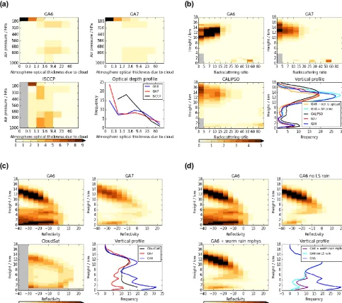
Tropics-wide (20◦N–20◦S) multi-annual average frequency histograms for ISCCP, CALIPSO and CloudSat, together with the outputs from COSP for GA6 and GA7 AMIP exper-iments, are shown in Fig. 2a–c. Taking ISCCP first (Fig. 2a), retrievals from passive instruments provide a cloud-top view. Compared with the newer active instruments, the vertical
resolution is poor and there are issues with the height as-signment under certain conditions (Mace and Wrenn, 2013). Nevertheless, the optical depth information from ISCCP re-mains valuable for optical depths greater than approximately 1.0, and hence an optical depth frequency profile is also shown. Both GA6 and GA7 tend to simulate too little cloud with intermediate optical thicknesses (1.0–10.0) and slightly too much optically thick cloud. Referring back to the full his-tograms, this bias appears to be the case for both high- and low-top cloud.
Arguably, CALIPSO provides the best global picture of total 2-dimensional cloud cover since, unlike the other in-struments considered here, it can detect thin sub-visual cir-rus. The vertical resolution is good; hence, in Fig. 2b, as well as providing the full histograms, we collapse along the backscattering ratio axis to provide a vertical profile of cloud frequency. In doing this, for altitudes below 4 km we only consider backscattering ratios greater than 5 due to the po-tential contamination from aerosols in the boundary layer; however, above 4 km backscattering ratios as low as 3 are in-cluded so as to account for very thin cirrus. This choice of the vertical profile of backscattering ratio threshold also gives a profile which most closely matches the CALIPSO cloud de-tection product used within the RL-GEOPROF dataset (Sup-plement Fig. S1). The lidar does become attenuated in the presence of thick ice cloud, and is attenuated quickly in the presence of liquid cloud, and hence this profile remains largely a cloud-top view.
Although the CloudSat radar is not sensitive to sub-visual cirrus, it uniquely provides a full 3-dimensional view of the cloud, only becoming attenuated in moderate and heavy rain. Despite the name, it should be noted that CloudSat is sen-sitive to precipitation as well as cloud. As for CALIPSO, in Fig. 2c we provide a vertical profile of hydrometeor fre-quency in addition to the full height–radar reflectivity his-tograms from CloudSat.
high-( a) ( b)
( c)
( d)
Figure 2.Tropical multi-annual mean observed and GA6- and GA7-simulated satellite data summaries.(a)ISCCP cloud-top pressure–optical depth joint frequency histograms. Lower right panel is a single optical depth frequency histogram (i.e. the joint histograms have been summed across cloud-top pressure bins). The threshold optical depth for detection by ISCCP is believed to be approximately 0.3, hence the masking of the lowest bin in the observed histogram.(b)CALIPSO backscattering ratio–frequency histograms by height. Lower right panel is a single height–frequency histogram (i.e. the backscattering ratio histograms have been summed across backscattering ratio bins in each height bin). Within the boundary layer, backscattering ratios<5 are likely to be due to aerosols (see Fig. S1) and hence are masked. The lower right panel also shows frequency profiles for GA6 with the cirrus spreading reduced to GA7 values, and GA6 but with the 6A convection scheme used.(c)CloudSat radar reflectivity (dBZ) and frequency histograms by height. Lower right panel is a single height–frequency histogram (i.e. the reflectivity histograms have been summed across reflectivity bins in each height bin).(d)As in(c)but showing GA6, GA6 without large-scale rain being passed to the simulator, and showing GA6 plus the warm rain microphysics package which is included in GA7. Colour scale for the histograms show frequency of occurrence of cloud or hydrometeor in the bin (%). Shading around the line plots has been added to reflect significance bounds; however, this is often less than the thickness of the plotted lines.
est cloud has the lowest backscattering ratios. This slight in-crease in the altitude of the cirrus is the result of the revised numerics of the convection scheme. This can be seen from the cyan line in Fig. 2b which is a simulation identical to GA6 (the blue line) but with the convection using the 6A scheme
(revised numerics). Despite this slight increase in height, the overall altitude of the thin cirrus still remains below that ob-served by CALIPSO.
(a)
(b)
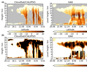
Figure 3.Case study of a GA6 6 h forecast verifying at 18:00 UTC on 17 December 2010 for an A-train pass over the South China Sea. (a)The observed and simulated radar reflectivities (dBZ) with situations in which the lidar detected cloud but the radar did not being included with a nominal value of−40 dBZ (e.g. Mace and Wrenn, 2013).(b)Observed and simulated cloud fraction on the model grid.
this example (which is typical of other convective cases ex-amined), the A-train overflew a convective system over the South China Sea. The top panels of Fig. 3 show the observed and GA6-simulated radar reflectivities. Data from CALIPSO have been added in locations where the lidar was detecting cloud which was not detected by the radar. It can be seen that the model is able to simulate thin cloud in the upper levels of the convective system right up to the observed altitudes of around 16 km. The nominal along-track resolution of the RL-GEOPROF product is 1.7 km, so if a threshold of−40 dBZ is used for cloud identification and it is regridded onto the model grid, which is 80 km near the equator, then an ob-served cloud fraction over a model grid box can be estimated. This assumes that the along-track cloud fraction is represen-tative of the 2-dimensional grid box. Whilst this is a fair as-sumption when considering a large number of cases which the A-train will cross at random orientations, there may be an error when considering a single case such as this. The ob-served and simulated grid-box cloud fraction on the model grid are shown in the lower panels of Fig. 3. Large cloud frac-tions occur up to the top of the convective system in the ob-servations, whereas they reduce quickly above 14 km in the model. So it appears that the lack of the highest thin cirrus is primarily because the fractional coverage of grid boxes is too small in situations where some cloud is present, rather than there being too many completely clear grid boxes at these altitudes. This is likely due to too little condensate being de-trained at these altitudes, with what is there being either the
result of convection going slightly deeper on occasional time steps or, more likely, some of the condensate being advected vertically having been detrained below.
Trade cumulus Stratocumulus
(a) (b)
(c) (d)
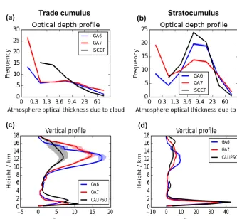
Figure 4.Observed and simulated multi-annual mean ISCCP optical depth frequency histograms(a, b)and CALIPSO height–frequency histograms(c, d)for a trade cumulus region (130–160◦W, 0–20◦S,a, c) and stratocumulus region (80–90◦W, 0–20◦S,b, d). Shading around the line plots has been added to reflect significance bounds; however, this is sometimes less than the thickness of the plotted lines.
out the Boutle et al. (2014) GCM upscaling; however, even after this correction, the auto-conversion rates remain around 10 times smaller than GA6, which accounts for the removal of the spurious drizzle.
Figure 3 shows, under the cirrus shield in GA6, an exten-sive region of high hydrometeor fraction and reflectivities of the order−10 dBZ, between the surface and 7 km which is absent in the observed transect. This is consistent with the region of the histogram in Fig. 2c where there is spurious large-scale rain. It is likely that large-scale cloud is forming in the moist air around the convective system and that it is undergoing auto-conversion, showing up as a strong signal in the CloudSat simulator. In GA7 (not shown) this precip-itation signal is removed with just a cloud signal remaining at around −40 dBZ. It should be noted that this is in a re-gion largely attenuated for CALIPSO as it is below the cirrus shield and so does not contribute to the “missing” mid-top cloud which is believed to be more cumulus congestus rather than large-scale cloud.
Tropical low cloud can be more easily assessed if re-gions are examined in which deep convection is rare or non-existent. Considering a region of the tropical Pacific domi-nated by trade cumulus, we found that GA6 appears to have too little cloud when compared with CALIPSO (Fig. 4a, c).
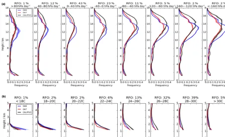
Figure 5. Observed and simulated CALIPSO height–frequency histograms composited by dailyω500 (a)and SST(b)over the tropics (20◦N–20◦S). Only the region below 5 km is shown in the lower plot to focus on low cloud. The range and relative frequency of occurrence (RFO) are shown at the top of each bin. Negativeω500indicates ascent. Shading around the line plots has been added to reflect significance bounds; however, this is sometimes less than the thickness of the plotted lines.
in GOCCP is smaller than 0.05 (Fig. 10 in Chepfer et al., 2013), supporting the interpretation that the cirrus amounts simulated by the models are excessive in this region.
Over the past couple of decades, a key focus of model de-velopment in the UM in relation to clouds has been on im-proving the simulation of subtropical stratocumulus due to its importance in determining the global cloud feedback under climate change (e.g. Bony and Dufresne, 2005). Many mod-els have too little cloud in this region, with what is there be-ing too bright (Nam et al., 2012). A number of improvements in previous configurations have resulted in the cloud amounts being in very good agreement with CALIPSO (Fig. 4b, d), although the low cloud amounts are reduced slightly in GA7 as a result of the change in the aerosol scheme to GLOMAP-mode. Compared with ISCCP, GA7 has considerably too lit-tle moderately reflective cloud in this region, but slightly too much optically thick cloud, indicating that what cloud is there remains too reflective. Consistent with this, compari-son against a number of observational datasets indicates that the cloud effective radius simulated by the model is too low in many regions, including subtropical stratocumulus (not shown), and is indicative of the aerosol cloud indirect effect being too strong (Walters et al., 2017b).
Compositing cloud data by large-scale variables is a use-ful way of summarizing the tropical cloud structures across
different meteorological situations. The most common are to composite against 500 hPa vertical velocity (Bony et al., 2004) and a measure of lower tropospheric stability. A num-ber of measures for the latter have been proposed (e.g. Klein and Hartmann, 1993; Williams et al., 2006; Wood and Bretherton, 2006); however, here we simply use the spacial variation in sea surface temperature (SST) (e.g. Williams et al., 2003). We composite the observed and modelled CALIPSO cloud profile by daily 500 hPa vertical velocity (ω500) and SST (Fig. 5). The desirable increase in altitude of the cirrus, discussed above for the tropics as a whole, can be seen in all the large-scale vertical velocity regimes. The re-duced cirrus amount in Fig. 2b is also reflected in Fig. 5, with the largest reduction in regions of strongest ascent. However, there now appears to be too little cirrus in weakly ascending regimes in GA7. This separation by regime therefore gives useful insights on where there might be compensating errors in the tropical mean picture provided by Fig. 2.
Figure 6.Distribution of average observed hydrometeor (cloud plus precipitation) fraction (colours) around a composite of ERA-I cyclones over Northern Hemisphere oceans for 5 years of DJF daily data. Panel(a)shows horizontal sections through the composite cyclone at 1.7 and 6 km with the mean PMSL contoured at 4 hPa intervals. Panel(b)shows vertical sections along the grey dashed lines shown in the top plots. Contours on the lower plots are mean vertical velocity from ERA-I (hPa d−1; negative values indicate ascent and these contours are dashed).
4 Cloud evaluation in the mid-latitude storm tracks
The weather over the mid-latitude oceans is characterized by the passage of synoptic systems. Since the cloud structures change on a daily basis, compositing of climatological data are essential. Here we follow Govekar et al. (2011) to analyse RL-GEOPROF cloud data around a composite cyclone, us-ing the cyclone compositus-ing technique of Field and Wood (2007). Cyclone centres are identified from daily ERA-I PMSL (pressure at mean sea level) data over the North-ern Hemisphere oceans (35–70◦N) and the RL-GEOPROF data extracted for a 30◦ latitude by 60◦longitude box cen-tred on the cyclone. All the cyclones from 5 years worth of daily December–January–February (DJF) data are then av-eraged to form a composite cyclone. In order to visualize the composite, Fig. 6 shows several sections through the 3-dimensional composite. The top panels are horizontal sec-tions in the boundary layer (1.7 km) and upper troposphere (6 km) with the mean PMSL contoured. The positions of frontal features will vary with time and between systems, and the size of cyclones varies, which also smooths the compos-ite, but on average it would be expected that fronts would occupy the south-east quadrant with a cloud head wrapping around the north of the cyclone (Field and Wood, 2007). This can be seen as higher cloud fractions in these locations in the section at 6 km, whilst the boundary-layer hydrometeor
fraction appears more symmetrical around the cyclone with a maximum near the centre. The lower panels in Fig. 6 are vertical sections across the composite to the south and to the east of the centre, with the contours indicating the average vertical velocity from ERA-I (dashed indicates ascent). The east–west cross section at 4◦south of the centre has large-scale descent in the cold air on the left of the plot, with cloud largely confined to the boundary layer. Moving to the east, there is a change to large-scale ascent and higher cloud frac-tions throughout the troposphere as we cross the composite warm conveyor belt. The north–south section shows similar strong ascent and high cloud fractions in the cloud head just to the north of the surface cyclone centre, but also an indi-cation of a secondary maximum at the southern end (−5◦, 2 km to−12◦, 6 km), where the section will sometimes pass through a trailing cold front.
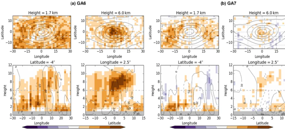
Figure 7.Cloud fraction absolute bias (model field minus observed field; colours) for composite cyclones. Produced as per Fig. 6 for(a) GA6 and(b)GA7, with the observed composite then subtracted. Black contours in top plots are the model mean PMSL and in the lower plots are the bias in vertical velocity. Student’st-test based on inter-annual variability shows that errors greater than 0.05 are statistically significant at the 0.05 level.
in GA7 through the reduced cirrus spreading rate, such that cloud amount biases in the free troposphere around the GA7 composite cyclone are very small.
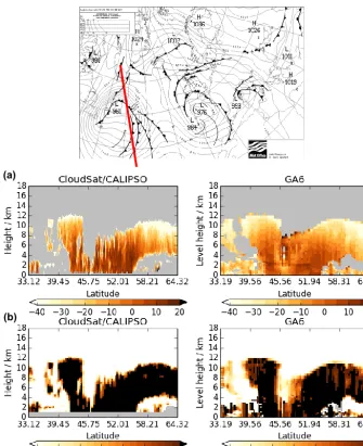
A case study again provides a useful illustration of the excess cirrus in GA6 (Fig. 8). In this example the A-train passed over a mature depression in a very similar section to the lower-right panel of the cyclone composite in Fig. 6. Given this is a forecast with a lead time greater than 1 day, the simulated positions of the frontal features are very good. The main bias is the width of the cloud associated with the warm conveyor belt being too large, which is especially vis-ible for the trailing cold front at around 44◦N. Examining the cloud fraction on the model grid, there are instances on the edges of the fronts where the observations suggest clear sky but the model simulates partially cloudy grid boxes. In contrast, within the cloud head around 60◦N, there is an in-dication that the model too readily breaks up the cloud when the grid box should be completely covered. This tendency for the model to too-often simulate partially cloudy grid boxes, rather than 0 % or 100 %, is consistent with previous experi-ence with the UM (e.g. Mittermaier, 2012) and may relate to the critical relative humidity which is still used to ini-tially form or decay cloud when the cloud-cover grid box is 0 %/100 %.
The same cyclone compositing methodology has been car-ried out over the Northern Hemisphere oceans for June–July– August (JJA) and for the summer and winter seasons in the Southern Hemisphere (40–70◦S). We have also composited anticyclones using the same cyclone settings as Field and Wood (2007), but testing ford2p/dx2+d2p/dy2<0 in
or-der to identify a local maximum in surface pressure rather than a local minimum. All the plots are available in the Sup-plement and show a broadly similar picture of excess cloud in the free troposphere and boundary layer in GA6, the former being essentially fixed and the latter improved in GA7. The GA6 cirrus biases in anticyclones are smaller than cyclones, but the boundary-layer errors are more similar. The cyclone composite for the Southern Hemisphere summer now sug-gests slightly too little mid-level (2–5 km) cloud on the cold-air side (poleward and westward side) of the cyclone in GA7 (Fig. S2). This may be associated with a lack of congestus cloud here, which is a long-standing problem but was being masked in GA6 through the excess cirrus throughout the free troposphere. Govekar et al. (2011) provided an evaluation of cyclone composite-cloud amounts over the Southern Ocean in an earlier configuration of the UM (Australian Community Climate and Earth System Simulator: ACCESS1.3). They concluded that while the cloud simulation was in reasonable agreement with observations, the large-scale vertical velocity was poor, and they cautioned that there may be a compensat-ing error in the cloud simulation. In both GA6 and GA7, the vertical velocities in the cyclone composites compare well with ERA-I (e.g. Fig. 7); hence, this issue is no longer of concern.
(a)
(b)
Figure 8.Case study of a GA6 27 h forecast verifying at 15:00 UTC on 16 February 2011 for an A-train pass over the North Atlantic, as shown by the red line on the synoptic analysis.(a)The observed and simulated radar reflectivities (dBZ) with situations in which the lidar detected cloud but the radar did not being included with a nominal value of−40 dBZ.(b)Observed and simulated cloud fraction on the model horizontal grid.
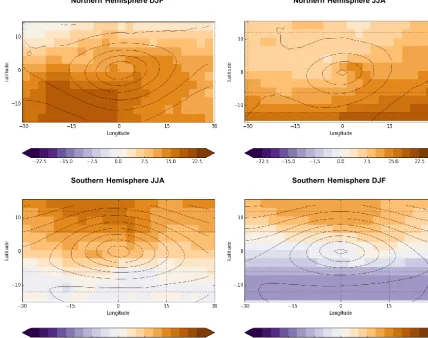
is in the reflected shortwave (RSW). Unsurprisingly, this er-ror is larger in the summer season in each hemisphere when the insolation is greatest. The Northern Hemisphere has ex-cess RSW across the cyclone composite, and particularly in regions of the composite that have more cloud. In contrast, the Southern Hemisphere has a large deficit of RSW on the cold-air side of the cyclone, a common bias in climate mod-els (Bodas-Salcedo et al., 2014). The Northern Hemisphere being too reflective can also be seen in the anticyclone com-posites (Fig. S4), but the Southern Hemisphere error seems mainly confined to the cyclone composite.
Figure 10 shows composite cyclone in-cloud albedo biases against ISCCP. In contrast to the RSW, the in-cloud albedo does not depend on the insolation, and so a cloud
Northern H emisphere DJF Northern H emisphere JJA
Southern H emisphere JJA Southern H emisphere DJF
(a) (b)
Figure 9.Cyclone composite GA7 mean bias in RSW and OLR (Wm−2) against CERES-EBAF (colours). Black contours are GA7 PMSL. Northern and Southern Hemisphere composites are shown for the respective winter(a)and summer(b)seasons. Student’st-test based on inter-annual variability shows that errors greater than 5 Wm−2are statistically significant at the 0.05 level.
not appear to be spatially well correlated with the RSW errors around the composite cyclone. We therefore suggest that mi-crophysical processes are primarily responsible for the SW errors through incorrect cloud albedos. This is a good exam-ple of the value of the compositing technique for understand-ing the likely cause of radiation errors. Although the subject of ongoing research, we believe that the negative in-cloud albedo bias on the cold-air side of the Southern Hemisphere cyclone is due to a lack of super-cooled liquid water (Bodas-Salcedo et al., 2016), whereas the Northern Hemisphere bias is thought to be associated with issues around the simulation of aerosols and their interaction with the clouds, particularly the strong cloud–aerosol interaction noted earlier.
5 Cloud evaluation over mid-latitude land
Much of the Northern Hemisphere mid-latitudes are land covered, and here we composite the RL-GEOPROF hydrom-eteor fraction and CALIPSO cloud fraction, along with their simulated equivalents, byω500. We illustrate the results for DJF (Fig. 11), although JJA is qualitatively similar. The ex-cess cirrus issue in GA6 can again be seen, and this is re-moved in GA7. For some of the regimes, it looks as though there may be now too little cirrus in GA7, although these are the relatively less populated regimes of strongest ascent and strongest subsidence.
There appears to be a significant excess of hydrometeor fraction in both model configurations at around 1 km; how-ever, the CALIPSO profiles suggest the cloud fractions at this level are generally correct. This exemplifies the utility of us-ing multiple observation types and indicates that the excess hydrometeor in the RL-GEOPROF comparison is low cloud in situations where there is thick high cloud above and/or ex-cess precipitation. Although a detailed investigation is yet to be carried out, it is suspected that both may be contributing. Case study analysis in the vicinity of the UK in February 2015 has identified a few occasions with spurious drizzle or light rain falling from stratocumulus (not shown). Unlike the warm-drizzle cases in the tropics which were improved by changes to the auto-conversion scheme in GA7, these mid-latitude winter cases have frozen cloud tops. It is possible that the microphysical errors leading to excess drizzle in frozen stratocumulus seen in the case study are a general issue con-tributing to the bias in Fig. 11. However, low cloud is fre-quently simulated by the model over land areas in the winter, and given that a cirrus shield is present on many occasions, it is quite possible that excess low cloud is also being simulated but shielded from the CALIPSO simulator.
Northern H emisphere DJF Northern H emisphere JJA
Southern H emisphere JJA Southern H emisphere DJF
Figure 10.Cyclone composite GA7 mean bias in in-cloud albedo (%) against ISCCP (colours). Black contours are GA7 PMSL.
the lowest cloud layers. Accurate predictions of cloud near the surface are of the highest importance for a number of users of the model, especially those in aviation. Here we use SYNOP data which, whilst having a reasonable global cov-erage over land, are likely to be the most reliable observation type available for this lowest layer. They avoid the ground clutter issues of remote sensing from space, and an upward-pointing ceilometer or a human observer looking from the ground are likely to achieve higher accuracy for low cloud bases as they avoid the problem of attenuation from cloud above. By looking at the lowest 1 km, many of the issues as-sociated with the SYNOP data (combining human and auto-mated data and differing observational errors associated with each) will be minimized (Mittermaier, 2012). In order to con-fine the analysis to cloud with bases below 1 km, we use the cloud-base height observation and look at frequency of oc-currence of cloud bases below 1 km. The cloud-base height is defined as the height of cloud with coverage of 3 oktas or more, and hence instances of small cloud coverage are excluded from this analysis. As a consequence, significant model biases in this diagnostic can appear if the observed cloud amount is typically just over 3 oktas and the model
cloud fraction is just under (or vice versa). This appears to be an issue for the UM in parts of the tropics where too little shallow cumulus is simulated and the model typically has cloud fractions of <3 oktas (i.e. grid-box fraction of
<0.375) whereas fractions over this threshold are often ob-served and hence a cloud-base height assigned. More gen-erally the diagnostic is reflecting errors in the frequency of occurrence of low-base cloud. Based on comparison with the active instruments at higher altitudes, we suspect that biases are more often reflecting errors in the frequency of occur-rence of low cloud rather than errors in the cloud-base height on any one occasion.
Figure 11.Observed and simulated RL-GEOPROF and CALIPSO height–frequency histograms composited by dailyω500over Northern Hemisphere land (polewards of 20◦N) during DJF. The range and relative frequency of occurrence (RFO) are shown at the top of each bin. Shading around the line plots has been added to reflect significance bounds; however, this is sometimes less than the thickness of the plotted lines.
most of the area, the model performs well and is essentially unbiased. Its performance over the UK is comparable to a 1.5 km convective permitting configuration of the UM, which is run operationally over the region (not shown). However, over areas of notable orography, such as the Alps, there ap-pears to be excess low cloud in the model. In contrast, around some of the coasts (especially France and Italy) there is too little low cloud. Further work is required to identify the cause of these errors.
6 Global cloud radiative effects
Traditionally the primary evaluation of clouds in climate models was carried out through an assessment of their im-pact on the TOA radiation budget. However, as discussed in the introduction, this could hide compensating errors which might result in an incorrect cloud radiative response to cli-mate change. We suggest instead that this assessment should be towards the end of a wider cloud evaluation, such as that presented above, feeding into the model development pro-cess.
Figure 12. Frequency bias ((hits+false alarms)/(hits+misses)) of cloud-base height<1 km for cloud fraction≥3 oktas in GA6 against surface station data. The mean bias of 6-hourly forecasts between 16 July 2014 and 15 July 2015 at a 24 h forecast lead time are shown.
some local improvements (e.g. in RSW over India and the equatorial Indian Ocean) and local detriments (e.g. in OLR over the Maritime Continent). A widespread bias for the free troposphere to be too cold in GA6 has been slightly improved in GA7 (mainly due to the introduction of the 6A convection scheme; Walters et al., 2017b), which largely accounts for the general increase in OLR in the newer model. Given that GA7 will be the physical model underpinning the UK submission to CMIP6, it is useful to compare to HadGEM2-A (Hadley Centre Global Environmental Model 2 – Atmosphere; Martin et al., 2011), which was the CMIP5 submission. It should be noted that HadGEM2-A is a comparatively old model with some 7 years of continuous model development having oc-curred between this and GA6, and hence the differences in the radiation budget are much larger. It can be seen that GA7 is a considerable improvement on HadGEM2, especially for the RSW. The error in the sub-tropical cumulus transition re-gions of excess RSW has been removed, and there is now a smaller negative bias in GA7. The lack of RSW over the Southern Ocean has been reduced by a third and RSW and OLR biases over the Maritime Continent have been signifi-cantly improved.
Metrics are often used to summarize the overall perfor-mance of the model. There are few such metrics in the liter-ature for NWP–seasonal cloud prediction applications; how-ever, a number have been proposed for aspects of the cloud simulation which are likely to be important for the radiative
response of cloud to climate change (e.g. Pincus et al., 2008; Klein et al., 2013; Myers and Norris, 2015). Here we illus-trate the calculation of metrics as the final step in the eval-uation process by presenting the present-day cloud regime error metric (CREMpd) of Williams and Webb (2009). This metric assesses the ability of the models to simulate pri-mary cloud regimes (as determined by the daily mean cloud cover, optical depth and cloud-top height) with the correct frequency of occurrence and radiative properties. Here we modify one aspect of the Williams and Webb (2009) ap-proach by using the newer global regimes proposed by Tse-lioudis et al. (2013) instead of calculating the tropics, extra-tropics, and snow- or ice-covered regions separately. Fig-ure 14 shows the CREMpd for GA6, GA7 and all the CMIP5 models for which the required data are available, with zero being a perfect score compared with the observations. GA6 is comparable with the previous HadGEM2-A model as it is also among the better-performing models on this metric, with GA7 performing slightly worse but still competitively with other CMIP5 models. Having a climate change appli-cation focus, CREMpd is very sensitive to the accuracy of the simulation of clouds with the strongest net radiative ef-fect, namely stratocumulus. Consequently GA7 is penalized compared with GA6 for the overall reduction in the albedo of sub-tropical stratocumulus (Fig. 4). In contrast, the met-ric has limited acknowledgment of the large improvements in the amount of cirrus in GA7 since the radiative effect of this largely sub-visual cloud is small.
7 Summary and discussion
(a)
(b)
Figure 13.Multi-annual mean bias in RSW(a)and OLR(b)(Wm−2) against CERES-EBAF for GA6, GA7 and HadGEM2-A. The spatial root-mean-square error (RMSE) is shown at the top of each panel.
Figure 14.Cloud regime error metric (CREMpd) from Williams and Webb (2009) for the global cloud regimes of Tselioudis et al. (2013), calculated for GA6 (blue), GA7 (red) and all of the CMIP5 models which have the required diagnostics available (black). Zero represents a perfect score with respect to the ISCCP observations.
RSW is likely due to errors in the in-cloud albedo rather than cloud amount; the use of surface-based observations for the lowest atmospheric layers where remote sensing from space becomes problematic; etc.
The combination of CloudSat and CALIPSO provides a unique 3-dimensional observational dataset of hydrometeor frequency through much of the atmosphere. We find that some care is required in its use for model evaluation in terms of separating cloud and precipitation, and the ability to perform multiple simulations passing different fields to the simulator can be valuable. Despite being an older satellite
dataset, the optical depth information from ISCCP remains extremely valuable for model evaluation purposes. Evalua-tion of very low cloud (<1 km) remains a challenge, espe-cially when thicker cloud exists above. We have made use of the SYNOP data which have reasonable coverage over land and, for cloud at these altitudes, may be regarded as fairly re-liable. The thresholds and variables available in the SYNOP data do limit the evaluation though.
of case studies in NWP hindcasts to understand the model errors at the process level. Although many centres do not routinely run simulations across these timescales, the AMIP and Transpose-AMIP experiments proposed by the Working Group Numerical Experimentation (WGNE) provide a rel-atively simple methodology, enabling all centres to benefit from this approach.
GA6 generally performs well given the critical examina-tion presented here. The main errors are as follows:
1. A considerable excess of thin, often sub-visual, cirrus erroneously extending from thicker cirrus clouds which ought to be present. This has been essentially fixed in GA7.
2. In-cloud albedo is too high in tropical and extra-tropical stratocumulus, except on the cold-air side of cyclones in the Southern Hemisphere, where they are too low. 3. A slight excess of boundary-layer hydrometeor fraction
over the mid-latitudes, which is suspected to be a com-bination of excess cloud and drizzle.
Apart from errors in external driving factors such as the lo-cation and timing of convection and synoptic systems, item 2 in the list above is the main cloud error affecting the mean radiation bias.
Although we have attempted the most comprehensive as-sessment possible in the time available, the task is inevitably open ended. The main omissions which we would have liked to address are an evaluation of the diurnal cycle of clouds globally and cloud over high-latitude regions. Sea ice and snow cover are likely to be quite sensitive to cloud, and this is a region which has generally received little detailed sys-tematic cloud evaluation. Use of data from additional instru-ments such as ground-based cloud radar and lidar, and from the Multi-angle Imaging Spectro-radiometer (MISR) satellite instrument would also be valuable additions in future studies.
Code availability. The UM is available for use under licence. A
number of research organizations and national meteorological ser-vices use the UM in collaboration with the Met Office to undertake basic atmospheric process research, produce forecasts, develop the UM code and build and evaluate Earth system models. For further information on how to apply for a licence see http://www.metoffice. gov.uk/research/collaboration/um-collaboration. Versions 8.6 (for GA6) and 10.3 (for GA7) of the source code are used in this pa-per. CERES EBAF data were obtained from the NASA Langley Re-search Center Atmospheric Science Data Center, at https://doi.org/ 10.5067/Terra+Aqua/CERES/EBAF-TOA_L3B.002.8. CALIPSO-GOCCP data were obtained from the IPSL ClimServ data centre http://climserv.ipsl.polytechnique.fr/cfmip-obs.html. CloudSat data were obtained from the CloudSat Data Processing Center http: //www.cloudsat.cira.colostate.edu/.
The Supplement related to this article is available online at https://doi.org/10.5194/gmd-10-2547-2017-supplement.
Competing interests. The authors declare that they have no conflict
of interest.
Acknowledgements. This work was supported by the Joint DECC–
Defra Met Office Hadley Centre Climate Programme (GA01101). We thank Cyril Morcrette, Paul Field and David Walters for useful discussions throughout the study.
Edited by: K. Gierens
Reviewed by: two anonymous referees
References
Abdul-Razzak, H. and Ghan, S. J.: A parameterization of aerosol ac-tivation: 2. Multiple aerosol types, J. Geophys. Res., 105, 6837– 6844, https://doi.org/10.1029/1999JD901161, 2000.
Baran, A. J., Cotton, R., Furtado, K., Havemann, S., Labon-note, L.-C., Marenco, F., Smith, A., and Thelen, J.-C.: A self-consistent scattering model for cirrus. II: The high and low frequencies, Q. J. R. Meteorol. Soc., 140, 1039–1057, https://doi.org/10.1002/qj.2193, 2014.
Beare, R. J.: The Role of Shear in the Morning Transi-tion Boundary Layer, Bound.-Lay. Meteorol., 129, 395–410, https://doi.org/10.1007/s10546-008-9324-8, 2008.
Bellouin, N., Rae, J., Jones, A., Johnson, C., Haywood, J., and Boucher, O.: Aerosol forcing in the Climate Model Intercom-parison Project (CMIP5) simulations by HadGEM2-ES and the role of ammonium nitrate, J. Geophys. Res., 116, D20206, https://doi.org/10.1029/2011jd016074, 2011.
Bodas-Salcedo, A., Webb, M. J., Bony, S., Chepfer, H., Dufresne, J. L., Klein, S., Zhang, Y., Marchand, R., Haynes, J. M., Pin-cus, R., and John, V. O.: COSP: satellite simulation software for model assessment, Bull. Am. Meteorol. Soc., 92, 1023–1043, https://doi.org/10.1175/2011BAMS2856.1, 2011.
Bodas-Salcedo, A., Williams, K. D., Ringer, M. A., Beau, I., Cole, J. N. S., Dufresne, J.-L., Koshiro, T., Stevens, B., Wang, Z., and Yokohata, T.: Origins of the solar radiation biases over the Southern Ocean in CFMIP2 models, J. Clim., 27, 41–56, https://doi.org/10.1175/JCLI-D-13-00169.1, 2014.
Bodas-Salcedo, A., Hill, P. G., Furtado, K., Williams, K. D., Field, P. R., Manners, J. C., Hyder, P., and Kato, S.: Large contribution of supercooled liquid clouds to the solar radia-tion budget of the Southern Ocean, J. Clim., 29, 4213–4228, https://doi.org/10.1175/JCLI-D-15-0564.1, 2016.
Bony, S. and Dufresne, J. L.: Marine boundary layer clouds at the heart of cloud feedback uncertainties in climate models, Geophys. Res. Lett., 32, L20806, https://doi.org/10.1029/2005GL023851, 2005.
com-ponents of cloud changes, Clim. Dynam., 22, 71–86, https://doi.org/10.1007/s00382-003-0369-6, 2004.
Boutle, I. A., Abel, S. J., Hill, P. G., and Morcrette, C. J.: Spa-tial variability of liquid cloud and rain: observations and mi-crophysical effects, Q. J. R. Meteorol. Soc., 140, 583–594, https://doi.org/10.1002/qj.2140, 2014.
Chepfer, H., Bony, S., Winker, D., Chiriaco, M., Dufresne, J.-L., and Sèze, G.: Use of CALIPSO lidar observations to evaluate the cloudiness simulated by a climate model, Geophys. Res. Lett., 35, L15704, https://doi.org/10.1029/2008GL034207, 2008. Chepfer, H., Bony, S., Winker, D., Cesana, G., Dufresne, J.-L.,
Min-nis, P., Stubenrauch, C. J., and Zeng, S.: The GCM Oriented Calipso Cloud Product (CALIPSO-GOCCP), J. Geophys. Res., 115, D00H16, https://doi.org/10.1029/2009JD012251, 2010. Chepfer, H., Cesana, G., Winker, D., Getzewich, B., Vaughan,
M., and Liu, Z.: Comparison of Two Different Cloud Climatologies Derived from CALIOP-Attenuated Backscat-tered Measurements (Level 1): The CALIPSO-ST and the CALIPSO-GOCCP, J. Atmos. Ocean. Technol., 30, 725–744, https://doi.org/10.1175/JTECH-D-12-00057.1, 2013.
Dee, D. P., Uppala, S. M., Simmons, A. J., Berrisford, P., Poli, P., Kobayashi, S., Andrae, U., Balmaseda, M. A., Balsamo, G., Bauer, P., Bechtold, P., Beljaars, A. C. M., van de Berg, L., Bid-lot, J., Bormann, N., Delsol, C., Dragani, R., Fuentes, M., Geer, A. J., Haimberger, L., Healy, S. B., Hersbach, H., Hölm, E. V., Isaksen, L., Kallberg, P., Köhler, M., Matricardi, M., McNally, A. P., Monge-Sanz, B. M., Morcrette, J. J., Park, P. K., Peubey, C., de Rosnay, P., Tavolato, C., Thêpaut, J. N., and Vitart, F.: The ERA-Interim reanalysis: configuration and performance of the data assimilation system, Q. J. R. Meteorol. Soc., 137, 553–597, https://doi.org/10.1002/qj.828, 2011.
Field, P. R. and Wood, R.: Precipitation and Cloud Struc-ture in Midlatitude Cyclones, J. Clim., 20, 233–254, https://doi.org/10.1175/JCLI3998.1, 2007.
Field, P. R., Heymsfield, A. J., and Bansemer, A.: Snow size distribution parameterization for midlatitude and tropical ice clouds, J. Atmos. Sci., 64, 4346–4365, https://doi.org/10.1175/2007JAS2344.1, 2007.
Field, P. R., Hill, A. A., Furtado, K., and Korolev, A.: Mixed-phase clouds in a turbulent environment, Part 2: An-alytic treatment, Q. J. R. Meteorol. Soc., 140, 870–880, https://doi.org/10.1002/qj.2175, 2014.
Flato, G., Marotzke, J., Abiodun, B., Braconnot, P., Chou, S. C., Collins, W., Cox, P., Driouech, F., Emori, S., Eyring, V., For-est, C., Gleckler, P., Guilyardi, E., Jakob, C., Kattsov, V., Rea-son, C., and Rummukainen, M.: Evalutation of climate mod-els, in: Climate Change 2013: The Physical Science Basis. Contribution of Working Group I to the Fifth Assessment Report of the Intergovernmental Panel on Climate Change, edited by: Stocker, T. F., Qin, D., Plattner, G.-K., Tignor, M., Allen, S. K., Boschung, J., Nauels, A., Xia, Y., Bex, V., and Midgley, P. M., Cambridge University Press, 741–866, https://doi.org/10.1017/CBO9781107415324.020, 2013. Gates, W.: The atmospheric model intercomparison project, Bull.
Am. Meteorol. Soc., 73, 1962–1970, 1992.
Gleckler, P. J., Taylor, K. E., and Doutriaux, C.: Performance metrics for climate models, J. Geophys. Res., 113, D06104, https://doi.org/10.1029/2007JD008972, 2008.
Govekar, P. D., Jakob, C., Reeder, M. J., and Haynes, J.: The three-dimensional distribution of clouds around Southern Hemi-sphere extratropical cyclones, Geophys. Res. Lett., 38, L21805, https://doi.org/10.1029/2011GL049091, 2011.
Haynes, J. M., Marchand, R. T., Luo, Z., Bodas-Salcedo, A., and Stephens, G. L.: A Multi-Purpose Radar Simulation Pack-age: QuickBeam, Bull. Am. Meteorol. Soc., 88, 1723–1727, https://doi.org/10.1175/BAMS-88-11-1723, 2007.
Khairoutdinov, M. F. and Kogan, Y. L.: A new cloud physics pa-rameterization in a large-eddy simulation model of marine stra-tocumulus, Mon. Weather Rev., 128, 229–243, 2000.
Klein, S. A. and Hartmann, D. L.: The Seasonal Cycle of Low Strat-iform Clouds, J. Clim., 6, 1587–1606, 1993.
Klein, S. A. and Jakob, C.: Validation and sensitivities of frontal clouds simulated by the ECMWF model, Mon. Weather Rev., 127, 2514–2531, 1999.
Klein, S. A., Zhang, Y., Zelinka, M. D., Pincus, R., Boyle, J., and Gleckler, P. J.: Are climate model simulations of clouds improv-ing? An evaluation using the ISCCP simulator, J. Geophys. Res., 118, 1329–1342, https://doi.org/10.1002/jgrd.50141, 2013. Loeb, N. G., Wielicki, B. A., Doelling, D. R., Kato, S.,
Wong, T., Smith, G. L., Keyes, D. F., and Manalo-Smith, N.: Toward Optimal Closure of the Earth’s Top-of-Atmosphere Radiation Budget, J. Clim., 22, 748–766, https://doi.org/10.1175/2008JCLI2637.1, 2009.
Mace, G. G. and Wrenn, F. J.: Evaluation of the hydrometeor layers in the east and west Pacific within ISCCP cloud-top pressure– optical depth bins using merged CloudSat and CALIPSO data, J. Clim., 26, 9429–9444, https://doi.org/10.1175/JCLI-D-12-00207.1, 2013.
Mace, G. G. and Zhang, Q.: The CloudSat radar-lidar ge-ometrical profile product (RL-GeoProf): Updates, improve-ments, and selected results, J. Geophys. Res., 119, 9441–9462, https://doi.org/10.1002/2013JD021374, 2014.
Mann, G. W., Carslaw, K. S., Spracklen, D. V., Ridley, D. A., Manktelow, P. T., Chipperfield, M. P., Pickering, S. J., and John-son, C. E.: Description and evaluation of GLOMAP-MODE: A modal global aerosol microphysics model for the UKCA composition-climate model, Geosci. Model Devel., 3, 519–551, https://doi.org/10.5194/gmd-3-519-2010, 2010.
Marchand, R., Mace, G. G., Ackerman, T., and Stephens, G. L.: Hydrometeor Detection Using Cloudsat – An Earth-Orbiting 94-GHz Cloud Radar, J. Atmos. Ocean. Technol., 25, 519–533, https://doi.org/10.1175/2007JTECHA1006.1, 2008.
Mittermaier, M.: A critical assessment of surface cloud observations and their use for verifying cloud forecasts, Q. J. R. Meteorol. Soc., 138, 1794–1807, https://doi.org/10.1002/qj.1918, 2012. Myers, T. A. and Norris, J. R.: On the relationships
be-tween subtropical clouds in meteorology in observations and CMIP3 and CMIP5 models, J. Clim., 28, 2945–2967, https://doi.org/10.1175/JCLI-D-14-00475.1, 2015.
Nam, C., Bony, S., Dufresne, J.-L., and Chepfer, H.: The ’too few, too bright’ tropical low-cloud problem in CMIP5 models, Geophys. Res. Lett., 39, L21801, https://doi.org/10.1029/2012GL053421, 2012.
Pincus, R., Batstone, C. P., Patrick-Hofmann, R. J., Taylor, K. E., and Gleckler, P. E.: Evaluating the present-day simulation of clouds, precipitation and radiation in climate models, J. Geophys. Res., 133, D14209, https://doi.org/10.1029/2007JD009334, 2008.
Rossow, W. B. and Schiffer, R. A.: Advances in understanding clouds from ISCCP, Bull. Am. Meteorol. Soc., 80, 2261–2287, 1999.
Stephens, G. L., Vane, D. G., Boain, R. J., Mace, G. G., Sassen, K., Wang, Z., Illingworth, A. J., O’Connor, E. J., Rossow, W. B., Durden, S. L., Miller, S. D., Austin, R. T., Benedetti, A., Mitrescu, C., and The CloudSat Science Team: The CloudSat mission and the A-Train, Bull. Am. Meteorol. Soc., 83, 1771– 1790, 2002.
Tselioudis, G., Rossow, W., Zhang, Y., and Konsta, D.: Global Weather States and their Properties from Passive and Ac-tive Satellite Cloud Retrievals, J. Clim., 26, 7734–7746, https://doi.org/10.1175/JCLI-D-13-00024.1, 2013.
Walters, D. N., Williams, K. D., Boutle, I. A., Bushell, A. C., Ed-wards, J. M., Field, P. R., Lock, A. P., Morcrette, C. J., Strat-ton, R. A., Wilkinson, J. M., Willett, M. R., Bellouin, N., Bodas-Salcedo, A., Brooks, M. E., Copsey, D., Earnshaw, P. D., Hardi-man, S. C., Harris, C. M., Levine, R. C., MacLachlan, C., Man-ners, J. C., Martin, G. M., Milton, S. F., Palmer, M. D., Roberts, M. J., Rodríguez, J. M., Tennant, W. J., and Vidale, P. L.: The Met Office Unified Model Global Atmosphere 4.0 and JULES Global Land 4.0 configurations, Geosci. Model Dev., 7, 361–386, https://doi.org/10.5194/gmd-7-361-2014, 2014.
Walters, D., Boutle, I., Brooks, M., Melvin, T., Stratton, R., Vosper, S., Wells, H., Williams, K., Wood, N., Allen, T., Bushell, A., Copsey, D., Earnshaw, P., Edwards, J., Gross, M., Hardiman, S., Harris, C., Heming, J., Klingaman, N., Levine, R., Man-ners, J., Martin, G., Milton, S., Mittermaier, M., Morcrette, C., Riddick, T., Roberts, M., Sanchez, C., Selwood, P., Stirling, A., Smith, C., Suri, D., Tennant, W., Vidale, P. L., Wilkinson, J., Willett, M., Woolnough, S., and Xavier, P.: The Met Office Unified Model Global Atmosphere 6.0/6.1 and JULES Global Land 6.0/6.1 configurations, Geosci. Model Dev., 10, 1487– 1520, https://doi.org/10.5194/gmd-10-1487-2017, 2017a. Walters, D. N., Baran, A., Boutle, I., Brooks, M. E., Furtado,
K., Hill, P., Lock, A., Manners, J., Morcrette, C., Mulchay, J., Sanchez, C., Smith, C., Stratton, R., Tennant, W., Van We-verberg, K., Vosper, S., Ashton, H., Essery, R., Gedney, N., Williams, K. D., and Zerroukat, M.: The Met Office Unified Model Global Atmosphere 7.0/7.1 and JULES Global Land 7.0 configurations, Geosci. Model Dev., in preparation, 2017b.
Webb, M., Senior, C., Bony, S., and Morcrette, J. J.: Combining ERBE and ISCCP data to assess clouds in the Hadley Centre, ECMWF and LMD atmospheric climate models, Clim. Dynam., 17, 905–922, 2001.
Williams, K. D. and Brooks, M. E.: Initial tendencies of cloud regimes in the Met Office Unified Model, J. Clim., 21, 833–840, https://doi.org/10.1175/2007JCLI1900.1, 2008.
Williams, K. D. and Tselioudis, G.: GCM intercompari-son of global cloud regimes: Present-day evaluation and climate change response, Clim. Dynam., 29, 231–250, https://doi.org/10.1007/s00382-007-0232-2, 2007.
Williams, K. D. and Webb, M. J.: A quantitative performance as-sessment of cloud regimes in climate models, Clim. Dynam., 33, 141–157, https://doi.org/10.1007/s00382-008-0443-1, 2009. Williams, K. D., Ringer, M. A., and Senior, C. A.: Evaluating the
cloud response to climate change and current climate variabil-ity, Clim. Dynam., 20, 705–721, https://doi.org/10.1007/s00382-002-0303-3, 2003.
Williams, K. D., Ringer, M. A., Senior, C. A., Webb, M. J., McA-vaney, B. J., Andronova, N., Bony, S., Dufresne, J.-L., Emori, S., Gudgel, R., Knutson, T., Li, B., Lo, K., Musat, I., Weg-ner, J., Slingo, A., and Mitchell, J. F. B.: Evaluation of a com-ponent of the cloud response to climate change in an inter-comparison of climate models, Clim. Dynam., 26, 145–165, https://doi.org/10.1007/s00382-005-0067-7, 2006.
Williams, K. D., Bodas-Salcedo, A., Deque, M., Fermepin, S., Medeiros, B., Watanabe, M., Jakob, C., Klein, S. A., Senior, C. A., and Williamson, D. L.: The Transpose-AMIP II ex-periment and its application to the understanding of Southern Ocean cloud biases in climate models, J. Clim., 26, 3258–3274, https://doi.org/10.1175/JCLI-D-12-00429.1, 2013.
Winker, D. M., Pelon, J., Coakley Jr, J. A., Ackerman, S. A., Charl-son, R. J., Colarco, P. R., Flamant, P., Fu, Q., Hoff, R. M., Kit-taka, C., Kubar, T. L., Treut, H. L., McCormick, M. P., Mégie, G., Poole, L., Powell, K., Trepte, C., Vaughan, M. A., and Wielicki, B. A.: The CALIPSO Mission: A Global 3D View of Aerosols and Clouds, Bull. Am. Meteorol. Soc., 91, 1211–1229, https://doi.org/10.1175/2010BAMS3009.1, 2010.
WMO: Guide to Meteorological Instruments and Methods of Ob-servation, Technical report WMO-8, World Meteorological Or-ganisation, Geneva, 2008.
Wood, R. and Bretherton, C. S.: On the relationship between strat-iform low cloud cover and lower tropospheric stability, J. Clim., 19, 6425–6432, 2006.