www.geosci-model-dev.net/9/4097/2016/ doi:10.5194/gmd-9-4097-2016
© Author(s) 2016. CC Attribution 3.0 License.
Multi-annual modes in the 20th century temperature variability in
reanalyses and CMIP5 models
Heikki Järvinen1, Teija Seitola1,2, Johan Silén2, and Jouni Räisänen1
1Department of Physics, University of Helsinki, Helsinki, Finland 2Finnish Meteorological Institute, Helsinki, Finland
Correspondence to:Heikki Järvinen ([email protected])
Received: 15 March 2016 – Published in Geosci. Model Dev. Discuss.: 24 March 2016 Revised: 7 October 2016 – Accepted: 25 October 2016 – Published: 17 November 2016
Abstract. A performance expectation is that Earth system models simulate well the climate mean state and the climate variability. To test this expectation, we decompose two 20th century reanalysis data sets and 12 CMIP5 model simula-tions for the years 1901–2005 of the monthly mean near-surface air temperature using randomised multi-channel sin-gular spectrum analysis (RMSSA). Due to the relatively short time span, we concentrate on the representation of multi-annual variability which the RMSSA method effectively cap-tures as separate and mutually orthogonal spatio-temporal components. This decomposition is a unique way to sepa-rate statistically significant quasi-periodic oscillations from one another in high-dimensional data sets.
The main results are as follows. First, the total spectra for the two reanalysis data sets are remarkably similar in all timescales, except that the spectral power in ERA-20C is sys-tematically slightly higher than in 20CR. Apart from the slow components related to multi-decadal periodicities, ENSO os-cillations with approximately 3.5- and 5-year periods are the most prominent forms of variability in both reanalyses. In 20CR, these are relatively slightly more pronounced than in ERA-20C. Since about the 1970s, the amplitudes of the 3.5-and 5-year oscillations have increased, presumably due to some combination of forced climate change, intrinsic low-frequency climate variability, or change in global observ-ing network. Second, none of the 12 coupled climate mod-els closely reproduce all aspects of the reanalysis spectra, although some models represent many aspects well. For in-stance, the GFDL-ESM2M model has two nicely separated ENSO periods although they are relatively too prominent as compared with the reanalyses. There is an extensive
Supple-ment and YouTube videos to illustrate the multi-annual vari-ability of the data sets.
1 Introduction
obtaining significance for the findings. Therefore, decadal-to-multi-decadal variability is of interest but not as informa-tive as focusing on shorter cycles of variability. Second, the applied methods have to be very effective in extracting in-formation from the short but high-dimensional data sets. For these reasons, we concentrate on the representation of multi-annual variability in reanalyses and coupled climate models applying randomised multi-channel singular spectrum anal-ysis (RMSSA; Seitola et al., 2014, 2015) which effectively separates mutually orthogonal spatio-temporal components from our high-dimensional data sets.
The aim of this study is to decompose the 20th century climate variability into its multi-annual modes, and to as-sess how these modes are represented by the contemporary climate models. We hope for this to provide guidance for model development due better understanding of the deficien-cies in representing reanalysed modes of multi-annual cli-mate variability. Ulticli-mately, interpretation of the hints about model deficiencies as development topics is due for the de-velopment teams themselves. Our role is to point towards the potential error sources. For reassuring the teams that high-dimensional time series analysis is possible today, we emphasise the methodological aspect of this study. RMSSA can, under very weak assumptions about the data, decom-pose high-dimensional data sets in a unique way and separate statistically significant quasi-periodic spatio-temporal oscil-lations from one another. This is in contrast to many other approaches which either make assumptions about the oscil-lation structures, such as Fourier or spherical decomposition, or resolve only either spatial or temporal aspects of variabil-ity. RMSSA can detect spatially evolving “chains of events” through resolving eigenmodes of spatio-temporal covariance data. This is a significant advantage over, say, PCA, which only resolves eigenmodes of spatial covariances and often projects temporal evolution of an “event” onto a number of different eigenmodes. In addition, the novel data compres-sion based on random projections enables here a vast increase in tractable problem size (i.e. data dimension) – even multi-variate decomposition is now possible, although not included here.
2 Methods and data
2.1 Randomised multi-channel singular spectrum analysis
Multi-channel singular spectrum analysis (MSSA; Broom-head and King, 1986a, b) can be characterised as being a time series analysis method for high-dimensional problems. It effectively identifies spatially and temporally coherent pat-terns of a data set by decomposing a lag-covariance data ma-trix into its eigenvectors and eigenvalues (e.g. Ghil et al., 2002) using singular value decomposition (SVD). The lag window in MSSA is a user choice, recommended typically
to be shorter than approximately one third of the length of the time series (Vautard and Ghil, 1989). A long lag win-dow enhances the spectral resolution, i.e. the number of fre-quencies that can be identified, but distributes the variance on a larger set of components. Here, MSSA eigenvectors are called space–time empirical orthogonal functions (EOFs), and the projections of the data set onto those ST-EOFs space–time principal components (ST-PCs). Because of the lag window, ST-PCs have a reduced length and they cannot be located into the same index space with the original time series. However, they can be represented in the origi-nal coordinate system by the reconstructed components (RC; Plaut and Vautard, 1994).
MSSA is computationally expensive and practical limits are easily exceeded for large data sets and long lag win-dows. In order to overcome this limitation, the computation-ally more efficient variant called RMSSA is applied here. The RMSSA algorithm, in a nutshell, (1) reduces the dimension of the original data set by using so-called random projections (RP; Bingham and Mannila, 2001; Achlioptas, 2003), (2) de-composes the data set by calculating standard MSSA in the low-dimensional space and (3) reconstructs the components in the original high-dimensional space.
In RP, the original data set is projected onto a matrix of Gaussian-distributed random numbers (zero mean and unit variance) in order to construct a lower dimensional represen-tation. In this study, we reduce the data volume to about 5 % of the original volume. Since the computational complex-ity of RP is low, involving only a matrix multiplication, it can be applied to very high-dimensional data sets. Although RP is not a lossless compression, it has the important prop-erty that the lower-dimensional data set has essentially the same structure as the original high-dimensional data set. This has been demonstrated for climate model data in Seitola et al. (2014). The RMSSA algorithm is briefly presented in the Appendix A.
2.2 Computation of spectra
The ST-PCs represent the different oscillatory modes ex-tracted from the data set. In order to estimate the dominant frequencies associated with each ST-PC, the power spectrum is calculated with the multitaper spectral analysis method (MTM) (Thomson, 1982; Mann and Lees, 1996). To further compare the variability modes and their intensities in differ-ent data sets, the power spectrum of all the ST-PCs of each data set is summed up to obtain so-called total spectrum. The ST-PCs are already weighted by their respective explana-tory power, i.e. multiplied by the corresponding eigenvalue. Therefore the components with more explanatory power also have higher spectral densities compared to the ones that ex-plain only a small fraction of the variance. Therefore no extra weighting is needed in this step.
eigen-value) is estimated using North’s rule of thumb for sampling errors (North et al., 1982). The sampling error(ek)is given byek∼λk(2/N ), whereλkis the eigenvalue associated with thekth ST-PC andN is the length of the time series. Thus, the confidence interval of the total spectrum describes the un-certainties related to the explanatory power of each ST-PC. 2.3 Statistical significance testing
In data sets of dynamical systems, ST-PCs/ST-EOFs of MSSA often appear as quadratic pairs that explain approxi-mately the same variance and areπ/2 out of phase with each other. However, the existence of such a pair does not guaran-tee any physical oscillation in the data set, and it may be due to some non-oscillatory processes, such as first-order autore-gressive noise. Allen and Robertson (1996) formulated a test, where the oscillatory modes identified with MSSA are tested against a red noise null hypothesis through Monte Carlo sim-ulation.
Significance testing in MSSA requires solving conven-tional PCs of the original data set. In case of very high-dimensional problems this easily exceeds practical compu-tational limits. The RMSSA implementation in Seitola et al. (2015) contains the Allen-Robertson test such that the PCs are solved in the dimension-reduced space, and is thus affordable even in very high-dimensional problems. The Ap-pendix A also includes a short description of the significance test.
2.4 Data sources
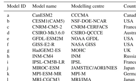
The data consist of the monthly mean near-surface air tem-perature from the historical 20th Century simulations of 12 different climate models (Table 1). The selected models originate from different modelling centres, and thus do not have close common-ancestor models. Furthermore, the se-lected models have undergone a long (generally several gen-erations) history of development, suggesting that the cho-sen models collectively reprecho-sent the state of the art. Near-surface temperature was chosen because many processes must be adequately represented in coupled models to realis-tically capture the observed temperature distribution (IPCC, 2013). These include processes in the Earth system compo-nent models (atmosphere, ocean, etc.) as well as in their mu-tual coupling models. Also, for the near-surface temperature, there are corresponding reanalysis data available.
The historical (1901–2005) simulations were extracted from the CMIP5 data archive and they follow the CMIP5 experimental protocol (Taylor et al., 2012). The 20th Cen-tury simulations use the historical record of climate forcing factors such as greenhouse gases, aerosols, solar variability, and volcanic eruptions. We used a single ensemble member of each model and the model data sets were interpolated into a common grid of 144×73 points.
Table 1.Climate models used in the study. For more details of the
models, see Table 9.1. in IPCC (2013).
Model ID Model name Modelling centre Country
a CanESM2 CCCMA Canada
b CESM1(CAM5) NSF-DOE-NCAR USA
c CNRM-CM5-2 CNRM-CERFACS France
d CSIRO-Mk3.6.0 CSIRO-QCCCE Australia
e GFDL-ESM2M NOAA GFDL USA
f GISS-E2-R NASA GISS USA
g HadGEM2-ES MOHC UK
h INM-CM4 INM Russia
i IPSL-CM5B-LR IPSL France
j MIROC-ESM JAMSTEC/AORI/NIES Japan
k MPI-ESM-MR MPI-M Germany
l MRI-CGCM3 MRI/JMA Japan
As a reference, we used two reanalysis data sets: the 20th Century Reanalysis V2 data (hereafter 20CR) provided by the NOAA/OAR/ESRL PSD (Compo et al., 2011), and ERA-20C data provided by ECMWF (Poli et al., 2013). The data sets are produced using an ensemble of perturbed reanaly-ses, and the final data set corresponds to the ensemble mean. In 20CR, only surface pressure observations are assimilated, and the observed monthly surface temperature and sea-ice distributions from HadISST1.1 (Rayner et al., 2003) are used as boundary conditions (Compo et al., 2011). In ERA-20C, observations of surface pressure and surface marine winds are assimilated (Poli et al., 2013). Unlike 20CR, it uses a more recent sea-surface temperature and sea-ice cover analysis from HadISST2 (Rayner et al., 2006). Both 20CR and ERA-20C are forced by historical record of changes in climate forcing factors (greenhouse gases, volcanic aerosols and solar variations). In order to be consistent with the cli-mate model simulations, the same time period is used (1901– 2005, i.e. 1260 monthly mean fields) and the reanalysis data sets were interpolated into the same grid as the model simu-lations (144×73 points).
2.5 Data processing
Some pre-processing of the data was needed before applying RMSSA. At each grid point the data sets were processed as follows:
– linear trend was fitted and removed,
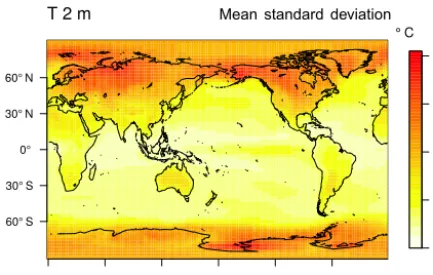
– annual cycle was estimated using seasonal-trend de-composition (STL; Cleveland et al., 1990) and removed, – resulting values were mean-centred and divided by the average standard deviation of all the data sets (see Fig. 1). Average standard deviation was obtained after removal of the trend and the annual cycle.
0 1 2 3 4
Mean standard deviation T 2 m
° C
00 60° E 120° E 180° 120° W 60° W 60° S
30° S 0° 30° N 60° N
°
Figure 1.Map of the common normalisation factor. Shown is the
mean standard deviation of 2 m temperature (◦C) across all the data sets.
temperature variability from inter-annual to multi-decadal timescales (e.g. Thompson et al., 2015). To retain these dif-ferences, we have used a common normalisation factor (i.e. the average standard deviation of all the data sets). This pro-cedure reduces the weight of grid points with high variance, typically at higher latitudes, and hence adds weight on the lower latitude features. After the pre-processing, the dimen-sion reduction step of RMSSA was applied so that approx-imately 5 % of the original data dimensions were retained. The lag window in the analysis was 20 years (240 months). The total spectra were obtained from this analysis, and are comparable due to normalisation using the common standard deviation of the data sets.
The statistical significance test uses a red noise null hy-pothesis. In the test we have used data sets that are nor-malised by their own standard deviations. Using a common normalisation interferes with generating the red noise sur-rogates corresponding to each data set. The first 50 PCs of each data set were retained as input. Those PCs explain 79 % of the variability in 20CR, 75 % in ERA-20C, and 70–80 % in the climate model data sets. A total of 1000 realisations of red noise surrogate data sets were generated, and confi-dence interval (95 %) for the oscillatory modes were esti-mated. We note that transformation to PCs may interfere with the detection of weak signals, as demonstrated by Groth and Ghil (2015).
2.6 Data visualisation
We used reconstructed components (RC; see Appendix A) for visualisation of the spatial patterns related to ST-PCs. For each grid point time series, we can calculate the RCs corre-sponding to the ST-PCs (or modes) of interest. These RC val-ues, reflecting the contribution of each grid point to the mode, can be plotted on a map at each time step. We have used these maps to construct videos of the spatio-temporal modes. In Sect. 3.5, we have analysed RCs corresponding to 3–4 year variability. The result is a time series of the data
correspond-ing to the 3–4 year mode in each grid point and accordcorrespond-ing to its variance after detrending and removing the annual cycle. In the analysis we have neglected 5 years in the beginning and the end of the time series, because the reconstruction pro-cedure may be biased there (see the Appendix, Eq. A4). The videos can be found at our YouTube channel (https://www. youtube.com/channel/UCu1zJdwJfLaXvfvTqsKCLHw).
To summarise the animations, we have calculated compos-ite maps of the modes. The compositing procedure follows the one described in Plaut and Vautard (1994). The idea is to choose the grid point time series (RCl) for which the
vari-ance is largest, and calculate its time derivative (RC0l). The phase of the mode at each time step is determined by calcu-lating the angle between the vector (RCl, RC0l) and the vector
(0,1). These phases, in the interval(0,2π ), are then classi-fied into eight equally populated categories. Composite maps are constructed from these categories.
3 Results
3.1 Reanalysis decompositions
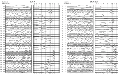
The main outcome of the RMSSA method, the space–time principal components (ST-PCs) characterise both the spa-tial and temporal structure of the modes of variability. Sec-tions 3.1–3.4 focus on their temporal aspects. The leading 30 ST-PC time series and the corresponding power spectra are displayed in Fig. 2 for 20CR and ERA-20C, ordered accord-ing to the explained variance. We can see that
– components with predominantly multi-decadal period-icity (1, 2, 5, and 6) explain a total of 7.2 and 5.9 % of the variance in 20CR and ERA-20C, respectively, with clear similarities in their time series and spectra; – multi-annual components (3, 4, 7, and 8) explain 4.2 and
3.2 % of the variance in 20CR and ERA-20C, respec-tively;
– there is a broad multi-annual peak centred at 5 years and a narrower peak at 3.5 years in both reanalyses; these are clearly separated in ERA-20C at the components 3 and 4 vs. 7 and 8. This separation in 20CR is less clear; – there are many spectral peaks in the reanalyses at 2–
3 year periods with little explained variance but some are well separated and distinct.
Explained
variance (%) Explainedvariance (%)
Period (yr) Period (yr)
70 50 30 20 10 5 4 3 2 1 70 50 30 20 10 5 4 3 2 1
1 2 3 4 5 6 7 8 9 10 11 12 13 14 15 16 17 18 19 20 21 22 23 24 25 26 27 28 29 30 1 2 3 4 5 6 7 8 9 10 11 12 13 14 15 16 17 18 19 20 21 22 23 24 25 26 27 28 29 30 2.4 1.9 0.9 0.9 0.8 0.8 0.7 0.7 0.7 0.7 0.6 0.6 0.6 0.5 0.5 0.5 0.4 0.4 0.4 0.4 0.4 0.4 0.4 0.4 0.4 0.4 0.3 0.3 0.3 0.3
70 50 30 20 10 5 4 3 2 1
1920 1940 1960 1980
3.0 2.1 1.2 1.1 1.1 1.0 1.0 0.9 0.9 0.8 0.7 0.7 0.7 0.7 0.7 0.6 0.6 0.6 0.5 0.5 0.5 0.5 0.5 0.5 0.4 0.4 0.4 0.4 0.4 0.4
70 50 30 20 10 5 4 3 2 1
1920 1940 1960 1980
20CR ERA-20C
Figure 2.Reanalysis ST-PC time series (columns 1 and 3) of monthly near-surface temperature 1901–2005 and their spectra (columns 2 and
4) for 20CR and ERA-20C. The components are ordered according to the explained variance (%).
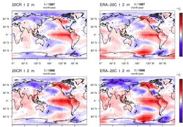
It is noteworthy in Fig. 2 that the components 3, 4, 7 and 8 in both reanalyses have become more prominent with time. Since about the 1970’s, the amplitudes of these 3.5- and 5-year oscillations have been at a higher level, presumably due to some combination of forced climate change, intrin-sic low-frequency climate variability, or changes in global observing networks (the rather sudden increase in the am-plitude seems to coincide with the onset of the modern era of satellite observations). This finding seems to be in support of e.g. Russell and Gnanadesikan (2014). In this connection it should be noted, however, that apparent low-frequency variations and changes in amplitude may simply arise from random fluctuations of the time series (Wunsch, 1999; Wittenberg, 2009). Back-projection of these compo-nents into the original grid representation (Fig. 3), reveals that the components are indeed associated with the ENSO phenomenon and are geographically similar in 20CR and ERA-20C. In the snapshots from January 1987 and Jan-uary 1998 (Fig. 3), there is a typical El Niño pattern with positive anomalies in the equatorial Pacific Ocean, South America, and northwestern North America. These are asso-ciated with synchronous evolution of (i) a dipole structure in the western Antarctica with easterly motion, and (ii) a wave-train type pattern in the northernmost North America with northeasterly motion. The components 3, 4, 7 and 8
thus represent a global phenomenon, with an increased am-plitude in recent decades. These features are nicely depicted on our YouTube channel (https://www.youtube.com/watch? v=vehbT8fOHeM, https://www.youtube.com/watch?v=xG– SiUqqAI).
3.2 Reanalysis total spectra
Figure 4a shows the total spectrum for the reanalyses con-structed from the ST-PCs, and their confidence intervals (dashed lines). As in the ST-PCs, there is most power in the slow modes. At periods of about 3.5- and 5-years, there are the spectral peaks of the components 3, 4, 7 and 8. The dip at 1 year reflects the removed annual cycle.
1 / 1998 20CR t 2 m
month/year
60° E 120° E 180° 120° W 60° W 60° S
30° S 0° 30° N 60° N
1 / 1987 20CR t 2 m
month/year
60° E 120° E 180° 120° W 60° W 60° S
30° S 0° 30° N 60° N
1 / 1998
0° 0°
0° 0°
−2
−1 0 1 2
ERA 20C t 2 m−
month/year °C
60° E 120° E 180° 120° W 60° W 60° S
30° S 0° 30° N 60° N
1 / 1987
−2
−1 0 1 2
ERA 20C t 2 m−
month/year °C
60° E 120° E 180° 120° W 60° W 60° S
30° S 0° 30° N 60° N
Figure 3.Global patterns of 2 m temperature for the components 3, 4, 7 and 8 in 20CR (left column) and ERA-20C (right column). Snapshots
are taken from January 1987 (top row) and January 1998 (bottom row). Unit◦C.
Statistical significance tests are presented in Figs. 4b and c for 20CR and ERA-20C, respectively. The multi-annual pe-riods (less than 7 years) rising above the 95 % confidence interval (i.e. the red dots above the region covered by the vertical bars) are 3.5, 3.6 and 5.7 years in 20CR and 3.6, 5.2, 5.5 and 5.7 years in ERA-20C. Thus, nearly the same peri-odicities rise above the red noise in the two data sets. It is logical that the frequency corresponding to the annual cycle is present in the red noise surrogates while it is absent from the data, and therefore the red dots fall far below their ex-pected values. Interestingly, the period of 2.9 years in 20CR and ERA-20C falls below the 95 % confidence interval. Our conclusion is therefore that the multi-annual climate variabil-ity in the near-surface air temperature is very similar in 20CR and ERA-20C.
3.3 CMIP5 model total spectra
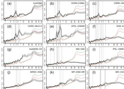
The total spectra for the 12 CMIP5 models are shown in Fig. 5 (solid lines) with their 95 % confidence intervals (dashed envelopes) and the reanalysis spectra as a reference (thin lines). Statistically significant multi-annual modes (at 5 % level) are denoted by vertical dashed lines. As in the case of reanalyses, these spectra are unique expressions of the low-frequency variability present in the simulation data. A comparison between the simulated and the reanalysis spectra provides one means to assess the strengths and weaknesses of these models. However, one cannot simply rank the models based on how “far off” the model spectra are from the
refer-ence, because this comparison focuses on just one (although important) aspect of model performance and because seem-ingly good agreement with observations might occasionally result from compensating errors in model processes.
Here we will concentrate on the multi-annual aspects but note in passing that the level of multi-decadal variability (>20 years) is close to reanalyses in models a, c, d, e, and g. In the rest of the models, the level seems too low. In the decadal scale (∼10. . . 20 years), the level of variance is close to reanalyses in a, b, c, f, i, j and l. Subjectively, the shape of the low-frequency end of the spectra appears most realistic in models a and c.
In multi-annual scales, the model performance varies a lot among the models. There is a group of models (a, b, d and e) with high spectral density at about 3–7 year periods. The models d and e have a bi-modal spectral structure, as in the reanalyses, while models a and b have a broad uni-modal peak. Decompositions (available in the Supplement, Sect. S1) partly explain the reasons leading to these total spectra.
5
10
20
50
100
Dominant period (years)
Eigen
value
1 2 3 4 5 7 10 20 30 50 70 100
20CR
(b)
5
10
20
50
100
Dominant period (years)
Eigen
value
1 2 3 4 5 7 10 20 30 50 70 100
ERA−20C
(c)
Period in years
Po
w
er
1e+5
5e+5
1e+6
1.5e+6
1 2 3 4 5 7 10 20 30 50 70 100
20CR
ERA−20C
(a)
Figure 4. (a) Total spectrum of 20CR (red line) and ERA-20C
(green line) with their min.–max. confidence intervals. The unit of the spectral density is arbitrary.(b)Significance of the 20CR pe-riodicities against red noise null hypothesis. Shown are the data eigenvalues (red squares) and the 2.5th and 97.5th percentiles of the eigenvalue distribution of the red noise surrogates (vertical bars).
(c)Same as(b), but for the ERA-20C data set.
the excessive spectral density at about 2 and 7–10 year peri-ods.
In model e, there is a bimodal total spectrum (Fig. 5e), although far too pronounced as compared with the reanaly-ses. The decomposition (Fig. S1e in the Supplement) reveals that the ST-PC components 1–10 (except 7–8) are all multi-annual and peak strongly and well in isolation at 3, 3.5, 4 and 5 years, explaining together no less than 13.9 % of the total variance. The development hint for model e is thus to investigate the mechanisms behind the components 1–10 and thereby obtain guidance for improving the realism of simu-lations.
In most other models, the multi-annual variability is less prominent than in the reanalyses. In model c (Fig. 5c), on the one hand, the decomposition points out (Fig. S1c in the Sup-plement) that there are about 12 ST-PC components with pe-riods between 1.5 and 3 years leading to a total spectrum with a broad peak of 2–3 year periods. These components tend to have very regular cycles, remotely resembling a coupled harmonic oscillator and seemingly missing the “offbeats” or
true quasi-periodicity of the reanalyses. The task seems to be to find out reasons why model c produces too-rapid and regular multi-annual variability. In model g (Fig. 5g), on the other hand, the leading ST-PC components 1–9 are on either decadal or multi-decadal periods and these overwhelm the to-tal spectrum. It should be important to find out the causes for this accentuated variability, especially on the decadal scale.
Finally, Fig. 5 casts light on models’ overall level of vari-ability compared to reanalyses. Clearly, this level in model h (Fig. 5h) is low. Curiously enough, the leading ST-PC com-ponent pair in model h explains only 1.4 % of variance and peaks at 3.2 year. This corresponds to the isolated peak in the total spectrum.
3.4 Significance of multi-annual modes in CMIP5 models
In the reanalyses (Fig. 4), only a few multi-annual periods rise above the red noise (three in 20CR and four in ERA-20C). They are at approximately 3.5- and 5-year periods. For the CMIP5 models, the test results are available in the Sup-plement (Sect. S2). In Fig. 5, the multi-annual modes with periods less than 7 years at the 5 % significance level are de-noted by dashed vertical lines.
In summary, there are 5–15 statistically significant peri-ods in the models, except for model k (Fig. 5k) with three and model g (Fig. 5g) with zero periods. The large num-ber of significant periods (models d and e, for instance) can be explained, at least partly, by the fact that the modes are quasi-periodic and the spectral density therefore appears on a range of frequencies. This manifests as an excursion of the red noise threshold on several adjacent frequencies. This is typical for models with large spectral power on certain timescales. In model l (Fig. 5l), for instance, there are two broad and distinct spectral peaks at about 3.5 and 6 year periods, and many significant periods are gathered at these and nearby frequencies. In contrast, models f and h (and to some extent model c) have several significant and distinct periods between 2 and 7 years. In terms of number of sig-nificant modes, models a, i, j and k seem to be closest to the reanalyses.
3.5 Spatial patterns of the 3–4 year mode
ST-PC components can be represented in the original coordi-nate system as so-called reconstructed components that can be visualised. In this section, some visualisation results are presented and discussed.
Amer-Period in years
1 2 3 4 5 10 20 30 50 70 100
1e+5
5e+5
1e+6
1.5e+6
1 2 3 4 5 7 10 20 30 50 70 100 CanESM2
(a)
Period in years
Po
w
er
1 2 3 4 5 10 20 30 50 70 100
1e+5
5e+5
1e+6
1.5e+6
1 2 3 4 5 7 10 20 30 50 70 100 CESM1(CAM5)
(b)
Period in years
Po
w
er
1 2 3 4 5 10 20 30 50 70 100
1e+5
5e+5
1e+6
1.5e+6
1 2 3 4 5 7 10 20 30 50 70 100 CNRM−CM5−2
(c)
Period in years
1 2 3 4 5 10 20 30 50 70 100
1e+5
5e+5
1e+6
1.5e+6
1 2 3 4 5 7 10 20 30 50 70 100 CSIRO−Mk3.6.0
(d)
Period in years
Po
w
er
1 2 3 4 5 10 20 30 50 70 100
1e+5
5e+5
1e+6
1.5e+6
1 2 3 4 5 7 10 20 30 50 70 100 GFDL−ESM2M
(e)
Period in years
Po
w
er
1 2 3 4 5 10 20 30 50 70 100
1e+5
5e+5
1e+6
1.5e+6
1 2 3 4 5 7 10 20 30 50 70 100 GISS−E2−R
(f)
Period in years
1 2 3 4 5 10 20 30 50 70 100
1e+5
5e+5
1e+6
1.5e+6
1 2 3 4 5 7 10 20 30 50 70 100 HadGEM2−ES
(g)
Period in years
Po
w
er
1 2 3 4 5 10 20 30 50 70 100
1e+5
5e+5
1e+6
1.5e+6
1 2 3 4 5 7 10 20 30 50 70 100 INM−CM4
(h)
Period in years
Po
w
er
1 2 3 4 5 10 20 30 50 70 100
1e+5
5e+5
1e+6
1.5e+6
1 2 3 4 5 7 10 20 30 50 70 100 IPSL−CM5B−LR
(i)
1 2 3 4 5 10 20 30 50 70 100
1e+5
5e+5
1e+6
1.5e+6
1 2 3 4 5 7 10 20 30 50 70 100 MIROC−ESM
(j)
Po
w
er
1 2 3 4 5 10 20 30 50 70 100
1e+5
5e+5
1e+6
1.5e+6
1 2 3 4 5 7 10 20 30 50 70 100 MPI−ESM−MR
(k)
Po
w
er
1 2 3 4 5 10 20 30 50 70 100
1e+5
5e+5
1e+6
1.5e+6
1 2 3 4 5 7 10 20 30 50 70 100 MRI−CGCM3
(l)
Figure 5.As Fig. 4a but now for each climate model (black line). The reanalysis spectra are shown as a reference (dashed green and red
lines). The dashed vertical lines indicate the climate model multi-annual periods significant at 5 % level.
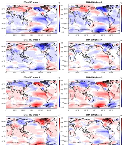
ica. Secondly, the mode contains tropical Pacific temperature anomalies, like in the ENSO phenomenon (e.g. Kleeman, 2008). The cold (warm) maximum is in phase 1 (5) with the anomalies extending to the South American continent. Thirdly, there are travelling temperature anomalies at high latitudes on both hemispheres. These are described next.
In phase 1 (Fig. 6), there is a small warm tempera-ture anomaly in the North Pacific (long 160◦W, lat 30◦N). This pattern slowly moves northeast, reaching Alaska in phase 5 and then gradually dissipating over northernmost North America in phase 8 (and being visible still in phase 1). There is a very similar evolution of a cold anomaly starting in phase 5. At the same time, there is an oscillating temperature anomaly over the Eurasian continent in the opposite phase. In Fig. 6, there is also a travelling temperature anomaly in the Southern Hemisphere. In phase 8 (Fig. 6), there is a cold anomaly over the Southern Ocean (long 160◦W). This strengthens, moves east, weakens, crosses the Antarc-tic Peninsula in phase 4 and remains in the Weddell Sea until phase 7. Similarly, there is a warm anomaly in phase 4 (long 160◦W) with similar evolution as the cold one.
Next, 20CR and the CMIP5 model behaviour is studied. The 3.5-year mode is significant in 20CR and ERA-20C. For the illustration, we have chosen component pairs from the model decompositions (Fig. S1 in the Supplement) that have spectral peaks between 3 and 4 years and do not express
sub-stantial variability on other timescales. In most climate mod-els, such a corresponding mode exists, except in models g and k. In model c this mode is not significant at 5 % level, but it is illustrated anyway. The Supplement reveals how these modes are represented in different data sets (Figs. S3–S14). The format is the same as in Fig. 6. A short summary is pre-sented next.
ERA−20C phase 1
−0.6 −0.4 −0.2 0.0 0.2 0.4 0.6
° C
0° 60°E 120°E 180° 120°W 60°W
60°S 30°S 0° 30°N 60°N
ERA−20C phase 2
−0.6 −0.4 −0.2 0.0 0.2 0.4 0.6
° C
0° 60°E 120°E 180° 120°W 60°W
60°S 30°S 0° 30°N 60°N
ERA−20C phase 3
−0.6 −0.4 −0.2 0.0 0.2 0.4 0.6
° C
0° 60°E 120°E 180° 120°W 60°W
60°S 30°S 0° 30°N 60°N
ERA−20C phase 4
−0.6 −0.4 −0.2 0.0 0.2 0.4 0.6
° C
0° 60°E 120°E 180° 120°W 60°W
60°S 30°S 0° 30°N 60°N
ERA−20C phase 5
−0.6 −0.4 −0.2 0.0 0.2 0.4 0.6
° C
0° 60°E 120°E 180° 120°W 60°W
60°S 30°S 0° 30°N 60°N
ERA−20C phase 6
−0.6 −0.4 −0.2 0.0 0.2 0.4 0.6
° C
0° 60°E 120°E 180° 120°W 60°W
60°S 30°S 0° 30°N 60°N
ERA−20C phase 7
−0.6 −0.4 −0.2 0.0 0.2 0.4 0.6
° C
0° 60°E 120°E 180° 120°W 60°W
60°S 30°S 0° 30°N 60°N
ERA−20C phase 8
−0.6 −0.4 −0.2 0.0 0.2 0.4 0.6
° C
0° 60°E 120°E 180° 120°W 60°W
60°S 30°S 0° 30°N 60°N
Figure 6.ERA-20C phase (1–8) composites of the 3–4 year variability mode. Unit◦C.
produce the North American pattern quite similar to reanaly-ses, and the northeast propagation is captured to some extent by models b, c, f, i and l.
4 Discussion
We note that a substantial portion of variance at inter-annual to inter-decadal timescales can be attributed to “cli-mate noise” associated with processes with timescales much shorter than the inter-annual scale (Wunsch, 1999; Feldstein,
5 Conclusions
The aim of this study is to decompose the 20th century cli-mate variability into its multi-annual modes, and to assess how these modes are represented by the contemporary cli-mate models. To this end, two 20th century reanalysis data sets and 12 CMIP5 model simulations for the years 1901– 2005 of the monthly mean near-surface air temperature have been decomposed using RMSSA. The statistical significance of the identified modes has been estimated with Monte Carlo simulations. The main conclusions are as follows.
Spectral properties of the 20CR and ERA-20C reanalysis data appear remarkably similar. The most prominent forms of variability in both data sets are related to approximately 3.5- and 5-year modes which are significant at 5 % level. The spectral power in ERA-20C is systematically slightly higher than in 20CR. The 3.5-year mode is illustrated in more detail. In ERA-20C, the mode is associated with a typical ENSO pattern of temperature anomalies in the equatorial Pa-cific Ocean, South America, and northwestern North Amer-ica. On top of these, the mode also contains a northeast-propagating temperature anomaly over northernmost North America, and another eastward-propagating anomaly in the vicinity of western Antarctica. Since about the 1970s, the amplitude of this 3.5-year global mode have increased.
None of the 12 coupled climate models closely reproduce all aspects of the reanalysis spectra, although some mod-els represent many aspects well. For instance, the GFDL-ESM2M model has two nicely separated ENSO-related peri-ods although they are relatively too prominent as compared to the reanalyses. Also, a number of models represent the propagating temperature anomalies at 3–4 year time frame. Some suggestions are provided in the text for potential model development aspects.
There is an extensive Supplement available presenting the results in visual format for each reanalysis and model data set. In the future, relaxation of the uni-variate nature of the present study would seem a natural extension. This is now possible since the use of random projections allows efficient data structures, preserving compression. Of special interest would be to study behaviour of variables directly linked with atmosphere–ocean coupling processes, such as heat, momen-tum and moisture fluxes over oceans.
6 Data and code availability
Appendix A: Randomised multi-channel singular spectrum analysis (RMSSA)
The RMSSA algorithm and the significance test is briefly presented here. The original data matrix isXN×L, where the columns are calledchannels. In case of gridded data set,N
represents the time steps andLis the number of grid points. It is useful to think of N as the time steps when the sam-pleof dimensionLis collected. The dimension reduction is a projectionXN×L→PN×k, whereLk. In other words, we preserve all samples but reduce the sample dimension from Ltok. The dimension reduction is performed in two steps: (1) generate a random matrixRL×k, where the matrix elements arerij ∼N (0,1)and column vectors ofRare nor-malised to unit length, and (2) projectXontoR:
PN×k=XN×LRL×k. (A1)
The next step is to construct an augmented data matrix A, which contains M lagged copies of each channel in P. In RMSSA, M represents the lag window.A now hasMk
columns andN0=N−M+1 rows. The singular value de-composition ofAis
A=UD1/2VT (A2)
The vectors ofUare the eigenvectors ofZ= 1
MkAA
T and VT contains the eigenvectors ofC= 1
N0ATA. These vectors
are orthogonal and often called space–time principal compo-nents (ST-PCs) and space–time empirical orthogonal func-tions (ST-EOFs), respectively. Note that the ST-EOFs are now in reduced space k. Diagonal elements of D are the eigenvalues ofCorZ. Finally, the eigenvectors (ST-EOFs) are calculated in the originalLdimensional space by
V≈AToU(D1/2)−1, (A3)
whereAois the augmented matrix of the original data matrix
X. Note that the calculation of ST-EOFs in Eq. (A3) can be limited only to the eigenmodes of interest.
The ST-PCs can be represented in the original coordinate system by the RCs (Plaut and Vautard, 1994; Ghil et al., 2002). This transformation is given by
rcle(n)= 1
Mn
Jn X
m=In
ue(n−m+1)vle(m), (A4)
whereueare the ST-PCs andvleare the ST-EOFs calculated in Eq. (A3) (the part of ST-EOF corresponding to channel
l).e is the index of the eigenmode that is calculated. The normalisation factorMn and the summation boundsIn and
Jn are given in Ghil et al. (2002) and for the central part of the time series(M≤n≤N−M+1)they are(M,1, M), respectively.
RMSSA with significance testing is briefly presented in the following. Testing the MSSA components against a red noise null hypothesis requires orthogonal input vec-tors, which are obtained by calculating first a conventional PCA and retaining a set of dominant PCs. Therefore some additional calculation steps are included in the RMSSA-algorithm:
SVD of lower dimensional matrixPis calculated to obtain the principal components (PCs, calculated as UD1/2). PCs fulfil the orthogonality constraint exactly. PCs, which explain a large part of the variance of the data set (e.g. 50 first), are retained to obtain matrixT, where the columns are the PCs. Next, the augmented matrixAPCis constructed fromTand
SVD is calculated as in Eq. (A2).
The Supplement related to this article is available online at doi:10.5194/gmd-9-4097-2016-supplement.
Author contributions. Heikki Järvinen suggested the study and mostly wrote the article. Teija Seitola implemented the meth-ods, performed all computations, and wrote data and method de-scriptions, Johan Silén supported the method development, and Jouni Räisänen the climate model data analysis.
Acknowledgements. This research has been funded by the Academy of Finland (project number 140771), Academy of Finland Centre of Excellence Programme (project number 272041) and the Fortum Foundation (grant number 201500127).
Edited by: R. Neale
Reviewed by: three anonymous referees
References
Achlioptas, D.: Database-friendly random projections: Johnson-Lindenstrauss with binary coins, J. Comput. Syst. Sci., 66, 671– 687, 2003.
Allen, M. R. and Robertson, A. W.: Distinguishing modulated os-cillations from coloured noise in multivariate datasets, Clim. Dy-nam., 12, 775–784, 1996.
Ba, J., Keenlyside, N. S., Latif, M., Park, W., Ding, H., Lohmann, K., Mignot, J., Menary, M., Otterå, O. H., Wouters, B., Salas y Melia, D., Oka, A., Bellucci, A., and Volodin, E.: A multi-model comparison of Atlantic multidecadal variability, Clim. Dynam., 9, 2333–2348, 2014.
Bellenger, H., Guilyardi, E., Leloup, J., Lengaigne, M., and Vialard, J.: ENSO representation in climate models: from CMIP3 to CMIP5, Clim. Dynam., 42, 1999–2018, 2014.
Bingham, E. and Mannila, H.: Random projection in dimensionality reduction: applications to image and text data, in: Proceedings of the seventh ACM SIGKDD international conference on Knowl-edge discovery and data mining, KDD’01, ACM, New York, 245–250, 2001.
Broomhead, D. S. and King, G. P.: Extracting qualitative dynamics from experimental data, Physica D, 20, 217–236, 1986a. Broomhead, D. S. and King, G. P.: On the qualitative analysis of
experimental dynamical systems, in: Nonlinear Phenomena and Chaos, edited by: Sarkar, S., Adam Hilger, Bristol, UK, 113–144, 1986b.
Cleveland, R. B., Cleveland, W. S., McRae, J. E.b and Terpenning, I.: STL: A Seasonal-Trend Decomposition Procedure Based on Loess, Journal of Official Statistics, 6, 3–73, 1990.
Compo, G. P., Whitaker, J. S., Sardeshmukh, P. D., Matsui, N., Al-lan, R. J., Yin, X., Gleason, B. E., Vose, R. S., Rutledge, G., Bessemoulin, P., Brönnimann, S., Brunet, M., Crouthamel, R. I., Grant, A. N., Groisman, P. Y., Jones, P. D., Kruk, M., Kruger, A. C., Marshall, G. J., Maugeri, M., Mok, H. Y., Nordli, Ø., Ross, T. F., Trigo, R. M., Wang, X. L., Woodruff, S. D., and Worley, S. J.: The Twentieth Century Reanalysis Project, Q. J. Roy. Meteor. Soc., 137, 1–28, doi:10.1002/qj.776, 2011.
Feldstein, S. B.: The timescale, power spectra, and climate noise properties of teleconnection patterns, J. Climate, 13, 4430–4440, 2000.
Fredriksen, H.-B. and Rypdal, K.: Spectral Characteristics of Instru-mental and Climate Model Surface Temperatures, J. Climate, 29, 1253–1268, doi:10.1175/JCLI-D-15-0457.1, 2016.
Ghil, M.: Natural climate variability, in: Encyclopedia of Global Environmental Change, edited by: Munn, T., Vol. 1, J. Wiley & Sons, Chichester/New York, 544–549, ISBN 0-471-97796-9, 2002.
Ghil, M., Allen, M. R., Dettinger, M. D., Ide, K., Kondrashov, D., Mann, M. E., Robertson, A. W., Saunders, A., Tian, Y., Varadi, F., and Yiou, P.: Advanced spectral methods for climatic time series, Rev. Geophys., 40, 1–41, 2002.
Groth, A. and Ghil, M.: Monte Carlo Singular Spectrum Analy-sis (SSA) Revisited: Detecting Oscillator Clusters in Multivariate Datasets, J. Climate, 28, 7873–7893, 2015.
IPCC (Flato, G., Marotzke, J., Abiodun, B., Braconnot, P., Chou, S. C., Collins, W., Cox, P., Driouech, F., Emori, S., Eyring, V., For-est, C., Gleckler, P., Guilyardi, E., Jakob, C., Kattsov, V., Reason, C., and Rummukainen, M.): Evaluation of Climate Models, in: Climate Change 2013: The Physical Science Basis. Contribution of Working Group I to the Fifth Assessment Report of the Inter-governmental Panel on Climate Change, edited by: Stocker, T. F., Qin, D., Plattner, G.-K., Tignor, M., Allen, S. K., Boschung, J., Nauels, A., Xia, Y., Bex, V., and Midgley, P. M., Cambridge University Press, Cambridge, United Kingdom and New York, NY, USA, 2013.
Järvinen, H., Seitola, T., Silén, J., and Räisänen, J.: Animations of the 3–4 year mode for all data sets, available at: https://www. youtube.com/channel/UCu1zJdwJfLaXvfvTqsKCLHw, last ac-cess: 16 November 2016.
Kleeman, R.: Stochastic theories for the irregularity of ENSO, Phi-los. T. R. Soc. A, 366, 2509–2524, 2008.
Knutson, T. R., Zeng, F., and Wittenberg, A. T.: Multimodel As-sessment of Regional Surface Temperature Trends: CMIP3 and CMIP5 Twentieth-Century Simulations, J. Climate, 26, 870– 8743, 2013.
Mann, M. E. and Lees, J. M.: Robust estimation of background noise and signal detection in climatic time series, Climatic Change, 33, 409–445, 1996.
Meehl, G. A., Goddard, L., Boer, G., Burgman, R., Branstator, G., Cassou, C., Corti, S., Danabasoglu, G., Doblas-Reyes, F., Hawkins, E., Karspeck, A., Kimoto, M., Kumar, A., Matei, D., Mignot, J., Msadek, R., Navarra, A., Pohlmann, H., Rienecker, M., Rosati, T., Schneider, E., Smith, D., Sutton, R., Teng, H., van Oldenborgh, G., Vecchi, G., and Yeager, S.: Decadal Cli-mate Prediction: An Update from the Trenches, B. Am. Meteo-rol. Soc., 95, 243–267, 2014.
North, G. R., Bell, T. L., Cahalan, R. F., and Moeng, F. J.: Sampling errors in the estimation of empirical orthogonal functions, Mon. Weather Rev., 110, 699–706, 1982.
Plaut, G. and Vautard, R.: Spells of low-frequency oscillations and weather regimes in the Northern Hemisphere, J. Atmos. Sci., 51, 210–236, 1994.
and initial performance evaluation of the ECMWF pilot re-analysis of the 20th-century assimilating surface observations only (ERA-20C), ERA Report Series, ECMWF, available at: http://www.ecmwf.int/en/research/climate-reanalysis/era-20c and http://www.ecmwf.int/en/elibrary/11699-data-assimilation- system-and-initial-performance-evaluation-ecmwf-pilot-reanalysis (last access: 14 November 2016), 2013.
Rayner, N. A., Parker, D. E., Horton, E. B., Folland, C. K., Alexan-der, L. V., Rowell, D. P., Kent, E. C., and Kaplan, A.: Global analyses of sea surface temperature, sea ice, and night marine air temperature since the late nineteenth century, J. Geophys. Res.-Atmos., 108, 446–469, 2003.
Rayner, N. A., Brohan, P., Parker, D. E., Folland, C. K., Kennedy, J. J., Vanicek, M., Ansell, T. J., and Tett, S. F. B.: Improved analyses of changes and uncertainties in sea surface temperature measured in situ since the mid-nineteenth century: The HadSST2 dataset, J. Climate, 19, 446–469, 2006.
Russell, A. M. and Gnanadesikan, A.: Understanding Multidecadal Variability in ENSO Amplitude, J. Climate, 27, 4037–4051, doi:10.1175/JCLI-D-13-00147.1, 2014.
Seitola, T., Mikkola, V., Silen, J., and Järvinen, H.: Random projec-tions in reducing the dimensionality of climate simulation data, Tellus A, 66, 25274, doi:10.3402/tellusa.v66.25274, 2014. Seitola, T., Silén, J., and Järvinen, H.: Randomised multichannel
singular spectrum analysis of the 20th century climate data, Tel-lus A, 67, 28876, doi:10.3402/telTel-lusa.v67.28876, 2015. Slingo, J. and Palmer, T.: Uncertainty in weather and climate
pre-diction, Philos. T. R. Soc. A., 369, 4751–4767, 2011.
Stevenson, S., Fox-Kemper, B., Jochum, M., Rajagopalan, B., and Yeager, S. G.: ENSO model validation using wavelet probability analysis, J. Climate, 23, 5540–5547, 2010.
Taylor, K. E., Stouffer, R. J., and Meehl, G. A.: An Overview of CMIP5 and the experiment design, B. Am. Meteorol. Soc., 93, 485–498, doi:10.1175/BAMS-D-11-00094.1, 2012.
Thomson, D. J.: Spectrum estimation and harmonic analysis, Proc. IEEE, 70, 1055–1096, 1982.
Thompson, D. W. J., Barnes, E. A., Deser, C., Foust, W. E., and Phillips, A. S.: Quantifying the role of internal climate variability in future climate trends, J. Climate, 28, 6443–6456, 2015. Vautard, R. and Ghil, M.: Singular spectrum analysis in nonlinear
dynamics, with applications to paleoclimatic time series, Physica D, 35, 395–424, 1989.
Wittenberg, A. T.: Are historical records sufficient to con-strain ENSO simulations?, Geophys. Res. Lett., 36, L12702, doi:10.1029/2009GL038710, 2009.