Coupling a three-dimensional subsurface flow and transport model with a land surface model to simulate stream–aquifer–land interactions (CP v1.0)

https://doi.org/10.5194/gmd-10-4539-2017 © Author(s) 2017. This work is distributed under the Creative Commons Attribution 3.0 License.

Coupling a three-dimensional subsurface flow and transport

model with a land surface model to simulate stream–aquifer–land

interactions (CP v1.0)

Gautam Bisht1, Maoyi Huang2, Tian Zhou2, Xingyuan Chen2, Heng Dai2, Glenn E. Hammond3, William J. Riley1, Janelle L. Downs4, Ying Liu2, and John M. Zachara5

1_{Earth & Environmental Sciences Division, Lawrence Berkeley National Laboratory, Berkeley, CA, USA}

2_{Atmospheric Sciences and Global Change Division, Pacific Northwest National Laboratory, Richland, WA, USA} 3_{Applied Systems Analysis and Research Department, Sandia National Laboratories, Albuquerque, NM, USA} 4_{Earth Systems Science Division, Pacific Northwest National Laboratory, Richland, WA, USA}

5_{Physical Sciences Division, Pacific Northwest National Laboratory, Richland, WA, USA} Correspondence:Maoyi Huang ([email protected])

Received: 8 February 2017 – Discussion started: 17 February 2017

Revised: 2 November 2017 – Accepted: 7 November 2017 – Published: 12 December 2017

Abstract. A fully coupled three-dimensional surface and subsurface land model is developed and applied to a site along the Columbia River to simulate three-way interactions among river water, groundwater, and land surface processes. The model features the coupling of the Community Land Model version 4.5 (CLM4.5) and a massively parallel mul-tiphysics reactive transport model (PFLOTRAN). The cou-pled model, named CP v1.0, is applied to a 400 m×400 m study domain instrumented with groundwater monitoring wells along the Columbia River shoreline. CP v1.0 simula-tions are performed at three spatial resolusimula-tions (i.e., 2, 10, and 20 m) over a 5-year period to evaluate the impact of hy-droclimatic conditions and spatial resolution on simulated variables. Results show that the coupled model is capable of simulating groundwater–river-water interactions driven by river stage variability along managed river reaches, which are of global significance as a result of over 30 000 dams con-structed worldwide during the past half-century. Our numer-ical experiments suggest that the land-surface energy parti-tioning is strongly modulated by groundwater–river-water in-teractions through expanding the periodically inundated frac-tion of the riparian zone, and enhancing moisture availability in the vadose zone via capillary rise in response to the river stage change. Meanwhile, CLM4.5 fails to capture the key hydrologic process (i.e., groundwater–river-water exchange) at the site, and consequently simulates drastically different water and energy budgets. Furthermore, spatial resolution is

found to significantly impact the accuracy of estimated the mass exchange rates at the boundaries of the aquifer, and it becomes critical when surface and subsurface become more tightly coupled with groundwater table within 6 to 7 me-ters below the surface. Inclusion of lateral subsurface flow influenced both the surface energy budget and subsurface transport processes as a result of river-water intrusion into the subsurface in response to an elevated river stage that in-creased soil moisture for evapotranspiration and suppressed available energy for sensible heat in the warm season. The coupled model developed in this study can be used for im-proving mechanistic understanding of ecosystem function-ing and biogeochemical cyclfunction-ing along river corridors under historical and future hydroclimatic changes. The dataset pre-sented in this study can also serve as a good benchmarking case for testing other integrated models.

1 Introduction

al., 2015), cloud formation (Rahman et al., 2015), and cli-mate (Leung et al., 2011; Taylor et al., 2013). Lateral sub-surface processes are fundamentally important on multiple spatial scales, including hill-slope scales (McNamara et al., 2005; Zhang et al., 2011), basin scales in semiarid and arid climates where regional aquifers sustain baseflows in rivers (Schaller and Fan, 2009) and wetlands (Fan and Miguez-Macho, 2011). However, some current-generation land sur-face models (LSMs) routinely omit explicit lateral subsursur-face processes (Clark et al., 2015; Kollet and Maxwell, 2008; Nir et al., 2014), while others include them (described below). Observational and modeling studies suggest that groundwa-ter forms an environmental gradient in soil moisture avail-ability by redistributing water that could profoundly shape critical zone evolution on continental to global scales (Fan et al., 2013; Taylor et al., 2013). The mismatch between ob-served and simulated evapotranspiration by current LSMs could be explained by the absence of lateral groundwater flow (Maxwell and Condon, 2016).

It has been increasingly recognized that rivers, despite their small aerial extent on the landscape, play important roles in watershed functioning through their connections with groundwater aquifers and riparian zones (Shen et al., 2016). The interactions between groundwater and river wa-ter prolong physical storage and enhance reactive processing that alter water chemistry, downstream transport of materials and energy, and biogenic gas emissions (Fischer et al., 2005; Harvey and Gooseff, 2015). The Earth system modeling community recognizes such a gap in existing Earth system models and calls for improved representation of biophysical and biogeochemical processes within the terrestrial–aquatic interface (Gaillardet et al., 2014).

Over the past decade, much effort has been expended to include groundwater in LSMs. Groundwater is impor-tant to water and energy budgets such as evapotranspira-tion (ET), latent heat (LH), and sensible heat (SH), but also to biogeochemical processes such as gross primary produc-tion, heterotrophic respiraproduc-tion, and nutrient cycling. The lat-eral convergence of water along the landscape and two-way groundwater–surface-water exchange are identified as the most relevant subsurface processes to large-scale Earth sys-tem functioning (see review by Clark et al., 2015). However, the choice of processes, the approaches to represent mul-tiscale structures and heterogeneities, the data and compu-tational demands, etc. all vary greatly among the research groups, even those working on the same land models.

Most of the LSMs reviewed by Clark et al. (2015) do not explicitly account for stream–aquifer–land interactions. For example, the Community Land Model version 4.5 allows for reinfiltration of flooded waters in a highly parameterized way without explicitly linking to groundwater dynamics, and therefore only one-way flow from the aquifer to the stream is simulated (Oleson et al., 2013). The Land–Ecosystem– Atmosphere Feedback model treats river elevation as part of the two-dimensional vertically integrated groundwater flow

equation and allows river and floodwater to infiltrate through sediments in the flood plain (Miguez-Macho and Fan, 2012). In contrast, the fully integrated models, being a small sub-set of LSMs, explicitly represent the two-way exchange be-tween groundwater aquifers and their adjacent rivers in a spa-tially resolved fashion. Such models couple a completely in-tegrated hydrology model with a land surface model, so that the surface-water recharge to groundwater by infiltration or intrusion and base flow discharge from groundwater to sur-face waters can be estimated in a more mechanistic way.

Examples of the integrated models include (1) the cou-pling between the Common Land Model (CoLM) and a variably saturated groundwater model (ParFlow) (Maxwell and Miller, 2005); (2) the Penn State Integrated Hydro-logic Model (PIHM) (Shi et al., 2013); (3) the coupling between the Process-based Adaptive Watershed Simulator (PAWS) and CLM4.5 (Ji et al., 2015; Pau et al., 2016; Ri-ley and Shen, 2014); (4) the coupling between the CATch-ment HYdrology (CATHY) model and the Noah model with multiple parameterization schemes (Noah-MP) (Niu et al., 2014); and (5) the coupling between CLM3.5 and ParFlow through the Ocean Atmosphere Sea Ice Soil external cou-pler (OASIS3) in the Terrestrial Systems Modeling Platform (TerrSysMP) (Shrestha et al., 2014; Gebler et al., 2017). The integrated models eliminate the need for parameteriz-ing lateral groundwater flow and allow the interconnected groundwater–surface-water systems to evolve dynamically based on the governing equations and the properties of the physical system. Although such models often require robust numerical solvers on high-performance computing (HPC) fa-cilities to achieve high-resolution, large-extent simulations (Maxwell et al., 2015), they have been increasingly applied for hydrologic prediction and environmental understanding. However, as a result of differences in physical process rep-resentations and numerical solution approaches in terms of (1) the coupling between the variably saturated groundter and surface wagroundter flow, (2) representation of surface wa-ter flow, and (3) implementation of subsurface hewa-terogene- heterogene-ity in the existing integrated models, significant discrepan-cies exist in their results when the models were applied to highly nonlinear problems with heterogeneity and complex water table dynamics, while many of the models show good agreement for simpler test cases where traditional runoff gen-eration mechanisms (i.e., saturation and infiltration excess runoff) apply (Kollet et al., 2017; Maxwell et al., 2014).

parameterizations in evaporation and transpiration, atmo-spheric boundary layer schemes) could have significant ef-fects on the simulations as well (Sulis et al., 2017). There-fore, it is of great scientific interest to further develop the in-tegrated models and benchmarks to achieve improved under-standing of complex interactions in the fully coupled Earth system.

Motivated by the great potentials of using an integrated model to explore Earth system dynamics, the objective of this study is three-fold. First, we aim to document the devel-opment of a coupled land surface and subsurface model as a first step toward a new integrated model, featuring the two-way coupling between two highly scalable and state-of-the-art open-source codes: CLM4.5 (Oleson et al., 2013) and a reactive transport model PFLOTRAN (Lichtner et al., 2015). The coupled model mechanistically represents the two-way exchange of water and solute mass between aquifers and river, as well as land–atmosphere exchange of water and en-ergy. The coupled model is therefore named as CP v1.0 here-after. We note that in recent years, efforts have been made to implement carbon–nitrogen decomposition, nitrification, denitrification, and plant uptake from CLM4.5 in the form of a reaction network solved by PFLOTRAN to enable the coupling of biogeochemical processes between the two mod-els (Tang et al., 2016). In addition, although PAWS is cou-pled to the same version of CLM (i.e., CLM4.5) (Ji et al., 2015; Pau et al., 2016), PFLOTRAN resolves the subsur-face in a three-dimensional fashion, while PAWS approxi-mates the three-dimensional Richards equation by dividing the subsurface into an unsaturated domain represented by the one-dimensional Richards Equation coupled with three-dimensional saturated groundwater flow equation for subsur-face flow, by assuming that there is no horizontal flow in an unsaturated portion of soil, and that lateral flux in saturated portion is evenly distributed.

Second, we describe a numerically challenging bench-marking case for verifying coupled land surface and sub-surface models, featuring a highly dynamic river boundary condition determined by dam-induced river stage variations (Hauer et al., 2017), representative of managed river reaches that are of global significance as a result of dam construc-tions in the past few decades (Zhou et al., 2016). Third, we assess the effects of spatial resolution and projected hydrocli-matic changes on simulated land surface fluxes and exchange of groundwater and river water using the coupled model and datasets from the benchmarking case. In Sect. 2, we describe the component models and our coupling strategy. In Sect. 3, we describe an application of the model to a field site along the Hanford reach of the Columbia River, where the subsur-face properties are well characterized and long-term mon-itoring of river stage, groundwater table, and exchange of groundwater and river water exist. In Sect. 4, we assess the effects of spatial resolution and hydroclimatic conditions to simulated fluxes and state variables. In Sect. 5, conclusions and future work are discussed.

2 Model description

2.1 The Community Land Model version 4.5

2.2 PFLOTRAN

PFLOTRAN is a massively parallel multiphysics simulator (Hammond et al., 2014) developed and distributed under an open-source GNU LGPL license and is freely available through Bitbucket (https://bitbucket.org/pflotran/pflotran). It solves a system of generally nonlinear partial differential equations (PDEs) describing multiphase, multicomponent, and multiscale reactive flow and transport in porous materi-als. The PDEs are spatially discretized using a finite-volume technique, and the backward Euler scheme is used for im-plicit time discretization. It has been widely used for simulat-ing subsurface multiphase flow and reactive biogeochemical transport processes (Chen et al., 2013, 2012; Hammond and Lichtner, 2010; Hammond et al., 2011; Kumar et al., 2016; Lichtner and Hammond, 2012; Liu et al., 2016; Pau et al., 2014).

PFLOTRAN is written in object-oriented Fortran 2003/2008 and relies on the PETSc framework (Balay et al., 2015) to provide the underlying parallel data structures and solvers for scalable high-performance computing. PFLOTRAN uses domain decomposition and MPI libraries for parallelization. PFLOTRAN has been run on problems composed of over 3 billion degrees of freedom with up to 262 144 processors, but it is more commonly employed on problems with millions to tens of millions of degrees of freedom utilizing hundreds to thousands of processors. Although PFLOTRAN is designed for massively parallel computation, the same code base can be run on a single processor without recompiling, which may limit problem size based on available memory.

In this study, PFLOTRAN is used to simulate single-phase variably saturated flow and solute transport in the subsurface. Single-phase variably saturated flow is based on the Richards equation with the form

∂

∂t(ϕsρ)+ ∇ ·ρq=0, (1)

with liquid densityρ, porosityφ, and saturations. The Darcy velocity,q, is given by

q= −kkr

µ ∇(p−ρgz) , (2)

with liquid pressurep, viscosityµ, acceleration of gravityg, intrinsic permeability k, relative permeabilitykr, and eleva-tion above a given datumz. Conservative solute transport in the liquid phase is based on the advection-dispersion equa-tion

∂

∂t(ϕsC)+ ∇ ·(q−ϕsD∇) C=0, (3)

with solute concentration C and hydrodynamic dispersion coefficient D. The discrete system of nonlinear PDEs for flow and transport are solved using the Newton–Raphson method.

2.3 Model coupling

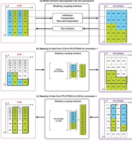
In this study, CLM4.5’s one-dimensional models for flow in unsaturated (Zeng and Decker, 2009) and saturated (Niu et al., 2007) zones are replaced by PFLOTRAN’s RICHRADS mode to simulate unsaturated–saturated flow within the three-dimensional subsurface domain. Although PFLOTRAN is also capable of simulating coupled flow and thermal processes in the subsurface, including explicit repre-sentation of liquid-ice phase (Karra et al., 2014) as well as soil nutrient cycles (Hammond and Lichtner, 2010; Zachara et al., 2016; Tang et al., 2016), those processes are not cou-pled between the two models in this study. A schematic representation of the coupling between CLM4.5 and PFLO-TRAN is shown in Fig. 1. A model coupling interface based on PETSc data structures was developed to couple the two models, and the interface includes some key design fea-tures of the CESM coupler (Craig et al., 2012). The model coupling interface allows each model grid to have a dif-ferent spatial resolution and domain decomposition across multiple processors. While CLM4.5 uses a round-robin composition approach, PFLOTRAN employs domain de-composition via PETSc (Fig. 1a). Interpolation of gridded data from one model onto the grids of the other is done through sparse matrix vector multiplication. As a prepro-cessing step, sparse weight matrices for interpolating data between the two models are saved as mapping files. Anal-ogous to the CESM coupler, the mapping files are saved in a format similar to the mapping files produced by the ESMF_RegridWeightGen (https://www.earthsystemcog.org/ projects/regridweightgen). ESMF regridding tools provide multiple interpolation methods (conservative, bilinear, and nearest neighbor) to generate the sparse weight matrix.

Figure 1.Schematic representations of the model coupling interface of CP v1.0.(a)Domain decomposition of a hypothetical CLM and PFLOTRAN domain comprising of 4×1×7 and 4×1×5 grids inx,y, andzdirections across two processors, as shown in blue and green.(b)Mapping of water fluxes from CLM onto PFLOTRAN domain via a local sparse matrix vector product for grids on processor 1. (c)Mapping of updated soil moisture from PFLOTRAN onto CLM domain via a local sparse matrix vector product for grids on processor 1.

stream–aquifer–land interactions are simulated in CP v1.0 when applied to the field scale, such as the 300 Area domain to be introduced in Sect. 3.1.

3 Site description and model configuration 3.1 The Hanford site and the 300 Area

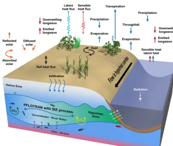
Figure 2.Schematic representation of hydrologic processes simulated in CP v1.0.

River above Priest Rapids Dam drains primarily mountain-ous regions in Canada, Idaho, Montana, and Washington, over which spatio-temporal distributions of precipitation and snowmelt modulate the timing and magnitude of river flows (Elsner et al., 2010; Hamlet and Lettenmaier, 1999). The Columbia River is highly regulated by dams for power gen-eration, and river stage and discharge along the Hanford Reach displays significant variation on multiple timescales. Strong seasonal variations occur, with the greatest discharge (up to 12 000 m3s−1)occurring from May through July due to snowmelt, with less discharge (> 1700 m3s−1)and lower flows occurring in the fall and winter (Hamlet and Letten-maier, 1999; Waichler et al., 2005). Significant variation in discharge also occurs on a daily or hourly basis due to power generation, with fluctuations in river stage of up to 2 m within a 6–24 h period being common (Tiffan et al., 2002).

The Hanford site features an unconfined aquifer developed in Miocene–Pliocene fluvial and lacustrine sediments of the Ringold Formation, overlain by Pleistocene flood gravels of the Hanford Formation (Thorne et al., 2006) that is in hydro-logic continuity with the Columbia River. The Hanford For-mation gravel and sand, deposited by glacial outburst floods at the end of the Pleistocene (Bjornstad, 2007), has a high average hydraulic conductivity at∼3100 m day−1(Williams et al., 2008). The fluvial deposits of the Ringold

Forma-tion have much lower hydraulic conductivity than those in the Hanford Formation but are still relatively conductive at 36 m day−1(Williams et al., 2008). Fine-grained lacustrine Ringold silt has a much lower estimated hydraulic conduc-tivity of 1 m day−1. The hydraulic conductivity of recent al-luvium lining the river channel is low relative to the Hanford Formation, which tends to dampen the response of water ta-ble elevation in wells near the river when changes occur in river stage (Hammond et al., 2011; Williams et al., 2008). Overall, the Columbia River through the Hanford Reach is a prime example of a hyporheic corridor with an extensive floodplain aquifer. It is consequently an ideal alluvial system for evaluating the capability of the coupled model in simu-lating stream–aquifer–land interactions.

teorological data representative of the general climatic con-ditions for the Hanford site.

A segment of the hyporheic corridor in the Hanford 300 Area was chosen to evaluate the model’s capability in simulating river–aquifer–land interactions. Located at the downstream end of the Hanford Reach, the impact of dam operations on river stage is relatively damped, exhibiting a typical variation of∼0.5 m within a day and 2–3 m in a year. The study domain covers an area of 400 m×400 m along the Columbia River shoreline (Fig. 3b). Aquifer sediments in the 300 Area are coarse-grained and highly permeable (Chen et al., 2013; Hammond and Lichtner, 2010). Coupled with dy-namic river stage variations, the resulting system is character-ized by stage-driven intrusion and retreat of river water into the adjacent unconfined aquifer system. During high-stage spring runoff events, river water has been detected in mon-itoring wells nearly 400 m from the shoreline (Williams et al., 2008). During baseline, low-stage conditions (October– February), the Columbia River is a gaining stream, and the aquifer pore space is occupied by groundwater.

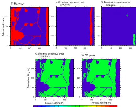
The study domain is instrumented with groundwater mon-itoring wells (Fig. 3b) and a river gaging station that records water table elevations. A vegetation survey in 2015 was con-ducted to provide aerial coverages of grassland, shrubland, and riparian trees in the domain (Fig. 3b). A high-resolution topography and bathymetry dataset at 1 m resolution was as-sembled from multiple surveys by Coleman et al. (2010). The data layers originated from deep-water bathymetric boat sur-veys, terrestrial light detection and ranging (lidar) sursur-veys, and special hydrographic lidar surveys penetrating through water to collect both topographic and bathymetric elevation data.

3.2 Model configuration, numerical experiments, and analyses

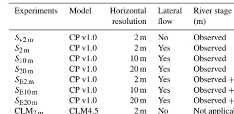
To assess the effect of spatial resolution on simulated vari-ables such as latent heat, sensible heat, water table depth, and river water in the domain, we configured CP v1.0 simu-lations at three horizontal spatial resolutions: 2, 10, and 20 m over the 400 m×400 m domain. For comparison purposes, we also configured a 2 m resolution CP v1.0 vertical-only simulation (i.e.,Sv2 m)in which lateral transfers of flow and solutes in the subsurface are disabled. Due to the lack of observations of water and energy fluxes from the land sur-face, in this study we treat the 2 m resolution CP v1.0 as the baseline and compare simulation results at other resolu-tions to it. New hydrologic regimes are projected to emerge over the Pacific Northwest as early as the 2030s due to in-creases in winter precipitation and earlier snowmelt in re-sponse to future warming (Leng et al., 2016a). Therefore, we expect that spring and early summer river discharge along the reach might increase in the future. To evaluate how land surface–subsurface coupling might be modulated hydrocli-matic conditions, we designed additional numerical

experi-Table 1.Summary of numerical experiments.

Experiments Model Horizontal Lateral River stage resolution flow (m)

S_{v2 m} CP v1.0 2 m No Observed

S_{2 m} CP v1.0 2 m Yes Observed

S_{10 m} CP v1.0 10 m Yes Observed

S20 m CP v1.0 20 m Yes Observed

S_{E2 m} CP v1.0 2 m Yes Observed+5

S_{E10 m} CP v1.0 10 m Yes Observed+5 S_{E20 m} CP v1.0 20 m Yes Observed+5

CLM_{2 m} CLM4.5 2 m No Not applicable

ments through driving the model with elevated river stages by adding 5 m to the observed river stage time series. The simulations and their configurations are summarized in Ta-ble 1.

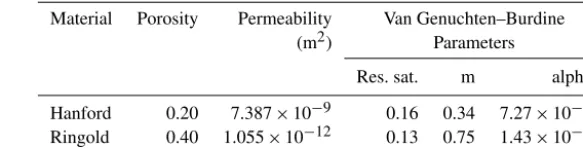
The PFLOTRAN subsurface domain, also terrain-following and extending from soil surface (including riverbed) to 32 m below the surface, was discretized us-ing a structured approach with rectangular grids. For the 2, 10, and 20 m resolution simulations, each mesh element was 2 m×2 m, 10 m×10 m, and 20 m×20 m in the hori-zontal direction and 0.5 m in the vertical direction, giving 2.56×106, 99.2×103, and 2.48×103 control volumes in total. The domain contained two materials with contrast-ing hydraulic conductivities: Hanford and Rcontrast-ingold (Fig. 4). Note that only the soil moisture and soil hydraulic proper-ties within the top 3.8 m are transferred from PFLOTRAN to CLM4.5 to allow simulations of infiltration, evaporation, and transpiration in the next time step, as the CLM4.5 sub-surface domain is limited to 3.8 m and cannot currently be easily modified. The hydrogeological properties of the Hanford and Ringold materials (Table 2) were taken from Williams et al. (2008). The unsaturated hydraulic conductiv-ity in PFLTORAN simulations was computed using the Van Genuchten water retention function (van Genuchten, 1980) and the Burdine permeability relationship (Burdine, 1953).

Table 2.Hydrogeological material properties of Hanford and Ringold materials. “Res. sat.” denotes residual saturation.

Material Porosity Permeability Van Genuchten–Burdine

(m2) Parameters

Res. sat. m alpha

Hanford 0.20 7.387×10−9 0.16 0.34 7.27×10−4 Ringold 0.40 1.055×10−12 0.13 0.75 1.43×10−4

(a) 2 m

(b) 10 m

(c) 20 m

Figure 4. PFLOTRAN meshes and associated material IDs at (a)2 m,(b)10 m, and(c)20 m resolutions.

A conductance value of 10−12_{m was applied to the} east-ern shoreline boundary to mimic the damping effect of low-permeability material on the river bed (Hammond and Licht-ner, 2010). A no-flow boundary condition was specified at the bottom of the domain to represent the basalt underlying the Ringold formation.

Vegetation types (Fig. 3b) were converted to correspond-ing CLM4.5 plant functional types (PFTs) and bare soil

(Fig. 5). At each resolution, fractional area coverages of PFTs and bare soil are determined based on the base map and written into the surface dataset as CLM4.5 inputs (Figs. 5, S1, and S2 in the Supplement). The CLM4.5 domain is terrain-following by treating the land surface as the top of the subsurface domain, which is hydrologically active to a depth of 3.8 m. The topography of the domain is retrieved from the 1 m topography and bathymetry dataset (Coleman et al., 2010) based on the North American Vertical Datum of 1988 (NAD88) and resampled to each resolution (Fig. S3).

The simulations were driven by hourly meteorological forcing from the Hanford meteorological stations and hourly river stage from the gaging station over the period of 2009– 2015. Precipitation, wind speed, air temperature, and rela-tive humidity were taken from the 300 Area meteorologi-cal station (46.578◦N, 119.726◦W) located∼1.5 km from the modeling domain. Other meteorological variables, such as downward shortwave and longwave radiation, were ob-tained from the Hanford Meteorological station (46.563◦N, 119.599◦W) located in the center of the Hanford site. The first 2 years of simulations (i.e., 2009 and 2010) were dis-carded as the spin-up period, so that 2011–2015 is treated as the simulation period in the analyses.

Among the hydroclimatic forcing variables (e.g., river stage, surface air temperature, incoming shortwave radia-tion, and total precipitation), river stage displayed the great-est interannual variability (Fig. 6). During the study period, high river stages occurred in early summer of 2011 and 2012 due to the melt of above-average winter snow packs in the upstream drainage basin, typical flow conditions oc-curred in 2013 and 2014, while 2015 was a year with low upstream snow accumulation. Meanwhile, the meteorolog-ical variables, especially temperature and shortwave radia-tion, do not show much interannual variability or changes in trends, while precipitation in late spring (i.e., May) of 2012 is higher than that in the other years, coincident with the high river stage in 2012. In the “elevated” experiments (i.e.,SE2 m, SE10 m, andSE20 m), the observed river stage (meters based on NAD88) was increased by 5 m at each hourly time step to mimic a perturbed hydroclimatic condition in response to future warming.

B

Figure 5.Plant function types at 2 m resolution as inputs for CLM4.5.

exchange (i.e.,S2 m andSE2 m)into two subdomains based on 2 m topography (shown in Fig. S3a): (a) the inland do-main where the surface elevation is higher than 110 m; and (b) the riparian zone where the surface elevation is less than or equal to 110 m. In addition to the latent heat flux, the evap-orative fraction, defined as the ratio of the latent heat flux to the sum of latent and sensible heat fluxes, was calculated over the subdomains for both observed and elevated condi-tions at a daily time step for all days with significant energy inputs (i.e., when net radiation is greater than 50 W m2). The evaporative fraction is an indicator of the type of surface, as summarized in literature (Lewis, 1995): it is typically less than 1 over surfaces with abundant water supplies; ranges be-tween 0.75 and 0.9, bebe-tween 0.5 and 0.7, and bebe-tween 0.15 and 0.3 for tropical rainforests, temperate forests and grass-lands, and semiarid landscapes, respectively; and approaches 0 over deserts.

To better quantify the spatio-temporal dynamics of stream–aquifer interactions, a conservative tracer with a mole fraction of one was applied at the river boundary to track the flux of river water and its total mass in the subsurface domain. While a constant concentration was maintained at

the river (i.e., eastern) boundary, the tracer was allowed to be transported out of the northern, western, and southern boundaries. Water infiltrating at the upper boundary based on CLM4.5 simulations was set to be tracer free, while a zero-flux tracer boundary condition was applied at the lower boundary. The initial flow condition was a hydrostatic pres-sure distribution based on the water table, as interpolated from the same set of wells that were used to create the tran-sient lateral flow boundary conditions at the northern, west-ern, and southern boundaries. The initial conservative tracer concentration was set to be zero for all mesh elements in the domain. The simulations were started on 1 January 2009 and the first 2 years were discarded as the spin-up period in the analysis. The mass of tracers in the domain and the fluxes of tracers across the boundary allow us to quantitatively un-derstand how river water is retained and transported in the subsurface domain.

-1

O

-Figure 6. Hydrometeorological drivers in the study period: (a) monthly mean river stage, (b) monthly total precipitation, (c)monthly mean surface air temperature, and(d)monthly mean incoming shortwave radiation.

note that CLM2 msimulations are not directly comparable to other simulations listed in Table 1 for the following reasons: (1) the CLM4.5 simulates subsurface hydrologic processes only down to 3.8 m below the surface, while the CP v1.0 sub-surface domain extends to∼30 m below the surface; (2) as discussed in Sect. 2.1, CLM4.5 uses TOPMODEL-based pa-rameterizations to simulate surface and subsurface runoffs, as well as mean groundwater table depth, using formulations derived from catchment hydrology that are only applicable at coarser resolutions; and (3) the key hydrologic processes (i.e., the exchange of river water and groundwater at the east-ern boundary and lateral transfer of water at all other bound-aries) that affect the hydrologic budget of the system are missing from CLM4.5. Therefore, the simulation was per-formed to characterize how physical parameterizations from one scale (i.e., catchment scale) affect simulations on another

scale (i.e., field scale) where those physical parameteriza-tions may not apply.

4 Results

4.1 Model evaluation

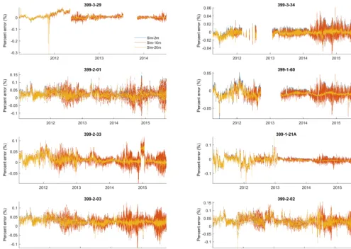
For the three-dimensional numerical experiments driven by the observed river stage time series (i.e.,S2 m,S10 m,S20 m), CP v1.0 simulated soil water pressure was converted to wa-ter table depth and compared against observed values at se-lected wells that were distributed throughout the domain and of variable distances from the river (Figs. 7, S4 and Table 3). The model performed very well in simulating the tempo-ral dynamics of the water table at all resolutions. The root-mean-square errors were 0.028, 0.028, and 0.023 m at 2, 10, and 20 m resolutions, respectively. The corresponding Nash– Sutcliffe coefficients were 0.998, 0.998, and 0.999. It was surprising that the performance metrics at 20 m resolution matches the observations better than those at finer resolu-tions, but the differences were marginal given the close match between the model simulation results and observations. River stage was clearly the dominant driving factor for water table fluctuations at the inland wells. In addition, errors in water and tracer budget conservations and surface energy conserva-tion for each time step inS2 mare shown in Fig. S5a, b, and c, respectively. The errors are sufficiently small when compared to the magnitudes of the related fluxes to ensure faithful sim-ulations in CP v1.0. These results indicated that the coupled model was capable of simulating dynamic stream–aquifer in-teractions in the near-shore groundwater aquifer that experi-ences pressure changes induced by river stage variations on subdaily timescales.

4.2 Effect of stream–aquifer interactions on land surface energy partitioning

Figure 7.Deviation (in percentages) of simulated water table levels from observations at selected wells shown in Fig. 3b.

Table 3. The comparison between simulated and observed water table levels.

Well S2 m S10 m S20 m

number RMSE N-S RMSE N-S RMSE N-S

(m) (m) (m)

399-3-29 0.022 0.999 0.022 0.999 0.021 0.999 399-3-34 0.011 1.000 0.011 1.000 0.006 1.000 399-2-01 0.039 0.997 0.038 0.997 0.029 0.998 399-1-60 0.016 1.000 0.016 0.999 0.013 1.000 399-2-33 0.028 0.998 0.028 0.998 0.022 0.999 399-1-21A 0.023 0.999 0.023 0.999 0.020 0.999 399-2-03 0.037 0.997 0.037 0.997 0.029 0.998 399-2-02 0.045 0.995 0.045 0.995 0.042 0.996

mean 0.028 0.998 0.028 0.998 0.023 0.999

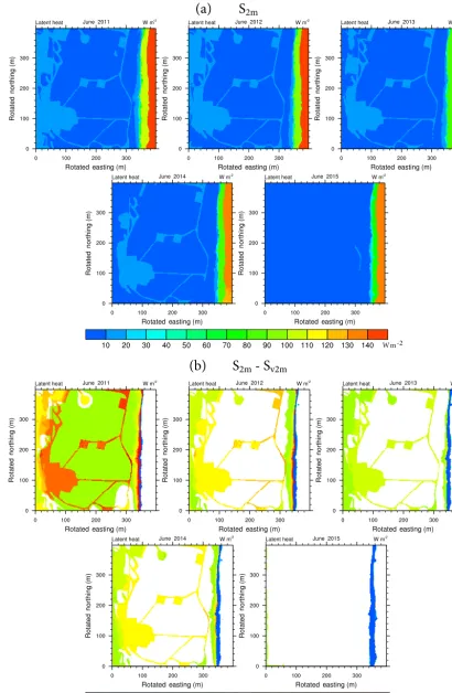
rabbitbrush and bunchgrass on the slope close to the river, are able to tap into the elevated water table with their deeper roots. In the inland portion of the domain, capillary supply was most evident in high-water years (i.e., 2011 and 2012), remains influential in normal years (i.e., 2013 and 2014), and

is essentially disabled in low-water years (i.e., 2015). The lateral discharge of shallow groundwater to the river led to a band of negative difference in LH betweenS2 mandSv2 mat the river boundary when the stage was low due to a decrease in rooting zone soil moisture for evapotranspiration by the ri-parian trees (Fig. 8b). This pattern was most evident in June 2015. Such a mechanism decreases in high-water and normal years because of more frequent inundation of the river bank and groundwater gradient reversal.

Figure 9.Difference between simulated latent heat fluxes bySE2 mandS2 min June.

ble level becomes shallower, a trend which is consistent be-tween the simulations (Fig. 10c). The daily evaporative frac-tions for the inland domain stayed well below 0.2 when the water table levels are less than 112 m, suggesting decoupled surface–subsurface conditions in a typical semiarid environ-ment. When water table levels increased to be above 112 m, the evaporative fraction increases to∼0.2, indicating that the surface and subsurface processes become more strongly cou-pled because of improved water availability for evapotran-spiration, especially in the elevated simulation (i.e., SE2 m). The evaporative fraction in the riparian zone remained close to 1.0, suggesting strong influences of the river and the role of deeper rooted plant types (e.g., riparian trees and shrubs) in modulating the energy partitioning (Fig. 10d) of riparian zones in the semiarid to arid environments.

To confirm the above findings, the liquid saturation (unit-less) and mass of river water (mol) in the domain fromS2 m andSE2 mon 30 June each year are plotted along a transect perpendicular to the river (y=200 m) in Figs. 11 and S6, and across ax–yplane at an elevation of 107 m in Figs. S7 and S8, respectively. Driven by the pressure introduced by elevated river stages, river water not only intruded further toward or even across the western boundary in high-water

years, but also led to a shallower water table and increased liquid saturation in the vadose zone due to capillary rise across the domain. In fact, liquid saturation in the shallow vadose zone could increase from 0.1–0.2 inS2 m to 0.3–0.4 inSE2 mon these days because of river-water intrusion. The river-water tracer could show up in the near-surface vadose zone at a distance of∼400 m from the river (Fig. S6). In-terestingly, by comparing the spatial distributions of river-water tracer in the low-river-water year (i.e., 2015) between the “observed” and “elevated” scenarios, the presence of river water in the domain was much less in the elevated scenario in terms of its spatial coverage (Figs. 11 and S6). This pat-tern suggests that after a number of years of enhanced river-water intrusion into the domain, the hydraulic gradient be-tween groundwater and river water could be reversed, so that groundwater discharging might be expected more frequently in low-water years in a prolonged elevated scenario.

Figure 10. Box plots of(a)land heat fluxes over the inland do-main and(b)latent heat fluxes in the riparian zone;(c)evaporative fractions over the inland domain;(d)evaporative fractions in the riparian zone in relation to groundwater table levels in the 5-year period. The blue boxes and whiskers represent summary statistics fromS2 m, and red ones indicate those fromSE2 m. The bottom and top of each box are the 25th and 75th percentile, the band inside the box is median, and the ends of the whiskers are maximum and minimum values.

As discussed in Sect. 2.1 and 3.2., the hydrologic param-eterizations in the default CLM4.5 model are based on con-ceptual and physical understandings from watershed hydrol-ogy that do not apply on the scale of our study site, where the exchange of river water and groundwater dominates the hydrologic budget of the system. Nevertheless, a compari-son between CLM4.5 and CP v1.0 helps characterize how scale inconsistencies in physical representations affect the simulations. Figure 12 shows comparisons of key compo-nents in the hydrologic budget between the two models. The simulated mean water table elevation of the domain from

CLM4.5 ranges between 74 and 80 m (i.e., 35–40 m below the surface), while the observed water table elevation ranges between 104 and 108 m (i.e., 5–10 m below the surface), and was accurately reproduced byS2 m(Fig. 12a). By using physics derived for the larger scale, CLM4.5 could not cap-ture subsurface river-water and groundwater exchanges, and consequently cannot accurately simulate groundwater table dynamics for our study domain.

At this semiarid field site, the groundwater and river-water exchanges represented in S2 m recharges the uncon-fined aquifer, and hence maintains sufficient soil water avail-ability in the top 3.8 m of the soil column, while the lack of groundwater and river-water interactions in CLM2 mleads to overall declining soil water content with seasonal variability as a result of percolation of winter rainwater (Fig. 12b). The difference in soil moisture availability propagates to evap-otranspiration (ET) and its components (Fig. 12c–f). Simu-lated summer ET in CLM2 m shows a high-frequency sig-nal in response to rainfall pulses through ground evapora-tion. Transpiration simulated by CLM2 m is determined by soil water availability in the soil column. In the spring and early summer of 2011 and 2013, transpiration from CLM2 m is close to that from S2 m given sufficient soil water. For other periods, CLM2 m simulates significant lower transpi-ration rates compared toS2 m.

Simulated latent heat fluxes in June for the period of 2011– 2015 from CLM2 m and their differences from those inS2 m are also illustrated in Fig. S9a and b. Evidently, the hydro-logic gradient from river to inland is missing as CLM4.5 lacks the capability of capturing the river stage dynamics at such a resolution (in Fig. S9a). Instead, although initiated from the same initial condition asS2 m on 1 January 2009 as discussed in the spin-up procedure in Sect. 3.2, soil mois-ture at the grid cells inundated or periodically inundated by the river is soon depleted through ET, surface runoff, or base-flow. However, latent heat from the inland domain is gener-ally higher in CLM2 mthan inS2 mdue to ground evaporation in response to rainfall pulses. In short, CLM4.5 fails to cap-ture the dynamics of groundwater and river-water exchanges. These biases propagate to simulated water and energy fluxes, which could have large impacts on boundary layer evolution, convection, and cloud formation in coupled land–atmosphere studies.

4.3 Effect of spatial resolution

simu-Figure 11.Liquid saturation levels (unitless) across a transect perpendicular to the river (y=200 m) on 30 June of each year in the study period from(a)S2 mand(b)SE2 m.

lated water table levels from the model were virtually identi-cal to observations. In this section, we further quantify biases of other variables of interest from the high-fidelity 2 m simu-lations.

The domain-averaged daily surface energy fluxes from S2 m show clear seasonal patterns, which are consistent in terms of their magnitudes and timing, reflecting mean cli-mate conditions at the site (Fig. S10). Driven by elevated river stages, latent heat fromSE2 mis consistently higher than that fromS2 m. The mean latent heat and sensible heat fluxes simulated by S2 m were 14.1 and 38.7 W m−2 over this

respec--2

-1

-1

-1

-1

O

Figure 12.Comparison of key hydrologic fluxes and state variables simulated by CLM_{2 m}andS2 m.

S S

S S

-Figure 13.Deviations of simulated domain-average latent heat and sensible heat fluxes from those simulated byS2 m (forS10 mand S_{20 m})and byS_{E2 m}(forS_{E10 m}andS_{E20 m}).

tively, compared to S2 m, but grew as large as 33.84 and 33.19 % forSE20 mandSE10 m, respectively, when compared toSE2 m. The 10 m simulations outperformed the 20 m sim-ulations under both scenarios but the magnitudes of errors were comparable. However, notably the vertical-only simu-lation (Sv2 m)has a small error of 5.67 % in LH compared to S2 m, indicating that lateral flow is less important when the water table is deep.

Figure 14.Deviations of total water mass, tracer, and exchange rates of water and tracer at four boundaries from those simulated byS2 m (forS10 mandS20 m)and bySE2 m(forSE10 mandSE20 m).

The results of simulations at three different resolutions in-dicated the following: (1) the partitioning of the land surface energy budget is mainly controlled by near-surface moisture – spatial resolution did not seem to be a significant factor in the computation of surface energy fluxes when the wa-ter table was deep at the semiarid site; (2) if the surface and subsurface are tightly coupled as in the elevated river stage simulations, resolution becomes an important factor to con-sider for credible simulations of the surface fluxes, as the land surface, subsurface, and riverine processes are expected to be more connected and coupled; (3) regardless of whether a tight coupling between the surface and subsurface occurs,

if mass exchange rates and associated biogeochemical reac-tions in the aquifer are of interest, a higher resolution is de-sired close to the river shoreline to minimize terrain errors.

5 Discussion and future work

Table 4.The relative error in surface energy fluxes simulated by S10 m and S20 m benchmarked against S2 m and by SE10 m and SE20 mbenchmarked againstSE2 m.

Simulation Latent heat Sensible heat flux (%) flux (%)

Sv2 m 5.67 1.63 S10 m 1.35 0.78 S20 m 2.41 1.42

SE10 m 33.19 13.71

SE20 m 33.84 14.18

Table 5.The relative error in total water mass and tracer amount in the subsurface simulated inS10 mandS20 mbenchmarked against S2 mand bySE10 mandSE20 mbenchmarked againstSE2 m.

Simulation Total water Total tracer

mass (%) (%)

S_{10 m} 0.03 5.44

S20 m 0.04 10.40

SE10 m 9.87 22.00

SE20 m 9.85 22.00

PFLOTRAN and the CLM4.5. Both models are under active development and testing by their respective communities, and therefore the coupled model could be updated to newer versions of PFLOTRAN and/or CLM to facilitate transfer of knowledge in a seamless fashion. The coupled model repre-sents a new addition to the integrated surface and subsurface suite of models.

By applying the coupled model to a field site along the Columbia River shoreline driven by highly dynamic river boundary conditions resulting from upstream dam opera-tions, we demonstrated that the model can be used to advance mechanistic understanding of stream–aquifer–land interac-tions surrounding near-shore alluvial aquifers that experi-ence pressure changes induced by river stage variations along managed river reaches, which are of global significance as a result of over 30 000 dams constructed worldwide during the past half-century. The land surface, subsurface, and riverine processes along such managed river corridors are expected to be more strongly coupled under projected hydroclimatic regimes as a result of increases in winter precipitation and early snowmelt. The dataset presented in this study can serve as a good benchmarking case for testing other coupled mod-els for their applications to such systems. More data need to be collected to facilitate the application and validation of the model to a larger domain for understanding the contri-bution of near-shore hydrologic exchange to water retention, biogeochemical cycling, and ecosystem functions along the river corridors.

By comparing simulations from the coupled model (CPv1.0) to that from CLM4.5, we demonstrated that the

catchment-scale physics imbedded in CLM4.5 does not ap-ply on the field scale. By misrepresenting, or not including, key hydrologic processes on the scale of interest, CLM4.5 fails to capture groundwater table dynamics, which could propagate to water and energy budgets and have profound impacts on boundary layer, convection, and cloud formation in coupled land–atmosphere studies. Our finding is consis-tent with results from other recent studies in which integrated surface and subsurface models were compared to standalone land surface models (Fang et al., 2017; Niu et al., 2017).

By benchmarking the coarser-resolution simulations at 20 and 10 m against the 2 m simulations, we find that resolution is not a significant factor for surface flux simulations when the water table is deep. However, resolution becomes impor-tant when the surface and subsurface processes are tightly coupled, and for accurately estimating the rate of mass ex-change at the riverine boundaries, which can affect the cal-culation of biogeochemical processes involved in carbon and nitrogen cycles.

Our numerical experiments suggested that riverine, land surface, and subsurface processes could become more tightly coupled through two mechanisms in the near-shore environ-ments: (1) expanding the periodically inundated fraction of the riparian zone and (2) enhancing moisture availability in the vadose zone in the inland domain through capillary rise. Both mechanisms can lead to increases in vadose-zone moisture availability and higher evapotranspiration rates. The latter is critical for understanding ecosystem functioning, biogeochemical cycling, and land–atmosphere interactions along river corridors in arid and semiarid regions that are ex-pected to experience new hydroclimatic regimes in a chang-ing climate. However, these systems have been poorly ac-counted for in current-generation Earth system models and therefore require more attention in future studies.

We acknowledge that there are a number of limitations of this study that need to be addressed in future studies.

1. In order to understand the stream–aquifer–land inter-actions with a focus on groundwater and river-water interactions along a river corridor situated in a semi-arid climate, the river boundary conditions were pre-scribed using observations with gaps filled by a one-dimensional hydrodynamics model. Future versions of the CP model need to incorporate two-way interactions between stream and aquifer by developing a surface flow component and testing the new implementation against standard benchmark cases (Kollet et al., 2017; Maxwell et al., 2014).

guaran-tee the validity of the Monin–Obukhov similarity theory (Arnqvist and Bergström, 2015). In our simulations, the majority of the Hanford 300 Area domain is covered by bare soil (z0=0.01 m), grass (z0=0.013 m), shrubs (z0=0.026–0.043 m), and riparian trees (varies across the seasons, z0=0.008 m when LAI=2 in the sum-mer andz0=1.4 when LAI=0 in the winter). There-fore, a 2 m resolution is sufficiently coarse under most conditions except for the grid cells covered by riparian trees in the winter. Nevertheless, the wintertime latent heat and sensible heat fluxes are nearly zero due to ex-tremely low energy inputs. Therefore, the 2 m simula-tions supported by the dense groundwater monitoring network at the site provide a valid benchmark for the coarser-resolution simulations. For future applications of the coupled model, caution should be taken to evalu-ate the site condition for the validity of model parame-terizations.

3. We used the simulated surface energy fluxes fromS2 m to verify coarser-resolution simulations. The simulated surface energy flux needs to be validated against eddy covariance tower observations, which are not available yet at the site. Nevertheless, we have made initial ef-forts to install eddy covariance systems at the site (see description in Sect. 3.1 of Gao et al., 2017), but the pro-cessing of the flux data is still preliminary. We will re-port flux observations and validations of the surface en-ergy budget simulations in future studies.

4. Even when observed fluxes are available for validation, the model structural problems associated with ET pa-rameterizations in CLM4.5 need to be addressed for rea-sonable simulations of the ET components, especially for the study site. That is, it has been well documented that ET simulated by CLM4.5 and CLM4 could be en-hanced when vegetation is removed. This ET enhance-ment over bare soil has been docuenhance-mented as a coun-terintuitive bias for most unsaturated soils in CLM4 and CLM4.5 simulations (Lawrence et al., 2012; Tang and Riley, 2013a). Tang and Riley (2013a) explored a few potential causes for this likely bias (e.g., soil resis-tance, litter layer resisresis-tance, and numerical time step). They found the implementation of a physically based soil resistance lowered the bias slightly, but concluded that the bias remained (Tang and Riley, 2013b). Mean-while, in studying ET over semiarid regions, Swenson and Lawrence (2014) proposed another soil resistance formulation to fix this excessive soil evaporation prob-lem within CLM4.5. While their modification improved the simulated terrestrial water storage anomaly and ET when compared to GRACE data and FLUXNET-MTE data, respectively, the empirical nature of the soil resis-tance proposed could have underestimated the soil re-sistance variability when compared to other estimates (Tang and Riley, 2013b).

Code and data availability. CLM4.5 (Oleson et al., 2013) is an open-source software released as part of the Community Earth System Model (CESM) version 1.2 (http://www.cesm.ucar.edu/models/cesm1.2). The version of CLM4.5 used in CP v1.0 is a branch from the CLM devel-oper’s repository. Its functionality is scientifically consistent with descriptions in Oleson et al. (2013) with source codes refactored for a modular code design. Additional minor code modifications were added by the authors to support coupling with PFLOTRAN (Lichtner et al., 2015). Permission from the CESM Land Model Working Group has been obtained to release this CLM4.5 development branch but the National Center for Atmospheric Research cannot provide technical support for this version of the code CP v1.0. PFLOTRAN is an open-source software distributed under the terms of the GNU Lesser General Public License, published by the Free Software Foundation as either version 2.1 of the license, or any later version. The CP v1.0 has two separate open-source repositories for CLM4.5 and PFLO-TRAN at https://bitbucket.org/clm_pflotran/clm-pflotran-trunk (commit hash: aff766d0f3d60db0b4983f5b06fd7fbc2f4f85e9) and https://bitbucket.org/clm_pflotran/pflotran-clm-trunk (com-mit hash: 1fa7da3ef8c976278644b39127b51819698ee698). The README guide for the CP v1.0 and dataset used in this study are available from the open-source repository https://bitbucket.org/pnnl_sbr_sfa/notes-for-gmd-2017-35.

The Supplement related to this article is available online at https://doi.org/10.5194/gmd-10-4539-2017-supplement.

Competing interests. The authors declare that they have no conflict of interest.

Acknowledgements. This research was supported by the US De-partment of Energy (DOE), Office of Biological and Environmental Research (BER), as part of BER’s Subsurface Biogeochemical Research Program (SBR). This contribution originates from the SBR Scientific Focus Area (SFA) at the Pacific Northwest National Laboratory (PNNL), operated by Battelle Memorial Institute for the US DOE under contract DE-AC05-76RLO1830. We greatly appreciate the constructive comments from two anonymous reviewers and the topical editor, Jatin Kala, which helped improve the paper significantly.

Edited by: Jatin Kala

Reviewed by: two anonymous referees

References

Arnqvist, J. and Bergström, H.: Flux-profile relation with roughness sublayer correction, Q. J. Roy. Meteor. Soc., 141, 1191–1197, https://doi.org/10.1002/qj.2426, 2015.

Zhang, H.: PETSc Users Manual, Tech. Rep. ANL-95/11 – Re-vision 3.5 Rep., Argonne National Laboratory, Lemont, Il, USA, 2015.

Basu, S. and Lacser, A.: A Cautionary Note on the Use of Monin–Obukhov Similarity Theory in Very High-Resolution Large-Eddy Simulations, Bound.-Lay. Meteorol., 163, 351–355, https://doi.org/10.1007/s10546-016-0225-y, 2017.

Beven, K. J. and Kirkby, M. J.: A physically based, vari-able contributing area model of basin hydrology/Un modèle à base physique de zone d’appel variable de l’hydrologie du bassin versant, Hydrol. Sci. B., 24, 43–69, https://doi.org/10.1080/02626667909491834, 1979.

Bjornstad, B. N.: On the Trail of the Ice Age Floods: A Geological Field Guide to the Mid-Columbian Basin, KeoKee, Sandpoint, ID, USA, 2007.

Burdine, N. T.: Relative Permeability Calculations From Pore Size Distribution Data, Journal of Petroleum Technology, 5, SPE-225-G, https://doi.org/10.2118/225-SPE-225-G, 1953.

Chen, X., Murakami, H., Hahn, M. S., Hammond, G. E., Rock-hold, M. L., Zachara, J. M., and Rubin, Y.: Three-dimensional Bayesian geostatistical aquifer characterization at the Hanford 300 Area using tracer test data, Water Resour. Res., 48, W06501, https://doi.org/10.1029/2011WR010675, 2012.

Chen, X., Hammond, G. E., Murray, C. J., Rockhold, M. L., Ver-meul, V. R., and Zachara, J. M.: Application of ensemble-based data assimilation techniques for aquifer characterization using tracer data at Hanford 300 area, Water Resour. Res., 49, 7064– 7076, https://doi.org/10.1002/2012WR013285, 2013.

Clark, M. P., Fan, Y., Lawrence, D. M., Adam, J. C., Bolster, D., Gochis, D. J., Hooper, R. P., Kumar, M., Leung, L. R., Mackay, D. S., Maxwell, R. M., Shen, C., Swenson, S. C., and Zeng, X.: Improving the representation of hydrologic processes in Earth System Models, Water Resour. Res., 51, 5929–5956, https://doi.org/10.1002/2015WR017096, 2015.

Coleman, A., Larson, K., Ward, D., and Lettrick, J.: Development of a High-Resolution Bathymetry Dataset for the Columbia River through the Hanford Reach Rep. PNNL-19878, Pacific North-west National Laboratory, Richland, WA, USA, 2010.

Condon, L. E., Maxwell, R. M., and Gangopadhyay, S.: The impact of subsurface conceptualization on land energy fluxes, Adv. Water Resour., 60, 188–203, https://doi.org/10.1016/j.advwatres.2013.08.001, 2013. Craig, A. P., Vertenstein, M., and Jacob, R.: A new

flex-ible coupler for earth system modeling developed for CCSM4 and CESM1, Int. J. High Perform. C., 26, 31–42, https://doi.org/10.1177/1094342011428141, 2012.

Elsner, M. M., Cuo, L., Voisin, N., Deems, J. S., Hamlet, A. F., Vano, J. A., Mickelson, K. E. B., Lee, S. Y., and Lettenmaier, D. P.: Implications of 21st century climate change for the hy-drology of Washington State, Climatic Change, 102, 225–260, https://doi.org/10.1007/s10584-010-9855-0, 2010.

Fan, Y. and Miguez-Macho, G.: A simple hydrologic framework for simulating wetlands in climate and earth system mod-els, Clim. Dynam., 37, 253–278, https://doi.org/10.1007/s00382-010-0829-8, 2011.

Fan, Y., Li, H., and Miguez-Macho, G.: Global Patterns of Ground-water Table Depth, Science, 339, 940–943, 2013.

Fang, Y., Leung, L. R., Duan, Z., Wigmosta, M. S., Maxwell, R. M., Chambers, J. Q., and Tomasella, J.: Influence of

land-scape heterogeneity on water available to tropical forests in an Amazonian catchment and implications for modeling drought response, J. Geophys. Res.-Atmos., 122, 8410–8426, https://doi.org/10.1002/2017JD027066, 2017.

Fischer, H., Kloep, F., Wilzcek, S., and Pusch, M. T.: A river’s liver – microbial processes within the hyporheic zone of a large low-land river, Biogeochemistry, 76, 349–371, 2005.

Gaillardet, J., Regnier, P., Lauerwald, R., and Ciais, P.: Geo-chemistry of the Earth’s surface GES-10 Paris France, 18–23 August, 2014, Carbon Leakage through the Terrestrial-aquatic Interface: Implications for the Anthropogenic CO₂ Budget, Proced. Earth Plan. Sc., 10, 319–324, https://doi.org/10.1016/j.proeps.2014.08.025, 2014.

Gao, Z., Russell, E. S., Missik, J. E. C., Huang, M., Chen, X., Strick-land, C. E., Clayton, R., Arntzen, E., Ma, Y., and Liu, H.: A novel approach to evaluate soil heat flux calculation: An ana-lytical review of nine methods, J. Geophys. Res.-Atmos., 122, 6934–6949, https://doi.org/10.1002/2017JD027160, 2017. Gebler, S., Hendricks Franssen, H. J., Kollet, S. J., Qu,

W., and Vereecken, H.: High resolution modelling of soil moisture patterns with TerrSysMP: A comparison with sensor network data, J. Hydrol., 547, 309–331, https://doi.org/10.1016/j.jhydrol.2017.01.048, 2017.

Gilbert, J. M., Maxwell, R. M., and Gochis, D. J.: Effects of Water-Table Configuration on the Planetary Boundary Layer over the San Joaquin River Watershed, California, J. Hydrometeorol., 18, 1471–1488, https://doi.org/10.1175/jhm-d-16-0134.1, 2017. Hamlet, A. F. and Lettenmaier, D. P.: Effects of climate change on

hydrology and water resources in the Columbia River basin, J. Am. Water Resour. As., 35, 1597–1623, 1999.

Hammond, G. E. and Lichtner, P. C.: Field-scale model for the natural attenuation of uranium at the Hanford 300 Area using high-performance computing, Water Resour. Res., 46, W09527, https://doi.org/10.1029/2009WR008819, 2010.

Hammond, G. E., Lichtner, P. C., and Rockhold, M. L.: Stochastic simulation of uranium migration at the Han-ford 300 Area, J. Contam. Hydrol., 120–121, 115–128, https://doi.org/10.1016/j.jconhyd.2010.04.005, 2011.

Hammond, G. E., Lichtner, P. C., and Mills, R. T.: Evaluating the performance of parallel subsurface simulators: An illustrative example with PFLOTRAN, Water Resour. Res., 50, 208–228, https://doi.org/10.1002/2012WR013483, 2014.

Harvey, J. and Gooseff, M.: River corridor science: Hydro-logic exchange and ecoHydro-logical consequences from bed-forms to basins, Water Resour. Res., 51, 6893–6922, https://doi.org/10.1002/2015WR017617, 2015.

Hauer, C., Siviglia, A., and Zolezzi, G.: Hydropeaking in regulated rivers – From process understanding to design of mitigation measures, Sci. Total Environ., 579, 22–26, https://doi.org/10.1016/j.scitotenv.2016.11.028, 2017.

Hou, Z., Huang, M., Leung, L. R., Lin, G., and Ricciuto, D. M.: Sensitivity of surface flux simulations to hydrologic parame-ters based on an uncertainty quantification framework applied to the Community Land Model, J. Geophys. Res.-Atmos., 117, D15108, https://doi.org/10.1029/2012JD017521, 2012. Hurrell, J. W., Holland, M. M., Gent, P. R., Ghan, S., Kay, J.

M., Bader, D., Collins, W. D., Hack, J. J., Kiehl, J., and Mar-shall, S.: The Community Earth System Model: A Framework for Collaborative Research, B. Am. Meteorol. Soc., 94, 1339– 1360, https://doi.org/10.1175/bams-d-12-00121.1, 2013. Ji, X., Shen, C., and Riley, W. J.: Temporal evolution of soil

moisture statistical fractal and controls by soil texture and re-gional groundwater flow, Adv. Water Resour., 86, 155–169, https://doi.org/10.1016/j.advwatres.2015.09.027, 2015. Karra, S., Painter, S. L., and Lichtner, P. C.: Three-phase

numer-ical model for subsurface hydrology in permafrost-affected re-gions (PFLOTRAN-ICE v1.0), The Cryosphere, 8, 1935–1950, https://doi.org/10.5194/tc-8-1935-2014, 2014.

Keune, J., Gasper, F., Goergen, K., Hense, A., Shrestha, P., Sulis, M., and Kollet, S.: Studying the influence of groundwater repre-sentations on land surface-atmosphere feedbacks during the Eu-ropean heat wave in 2003, J. Geophys. Res.-Atmos., 121, 13301– 13325, https://doi.org/10.1002/2016JD025426, 2016.

Kollet, S. J. and Maxwell, R. M.: Capturing the influence of ground-water dynamics on land surface processes using an integrated, distributed watershed model, Water Resour. Res., 44, W02402, https://doi.org/10.1029/2007WR006004, 2008.

Kollet, S. J., Sulis, M., Maxwell, R. M., Paniconi, C., Putti, M., Bertoldi, G., Coon, E. T., Cordano, E., Endrizzi, S., Kikinzon, E., Mouche, E., Mügler, C., Park, Y.-J., Refsgaard, J. C., Stisen, S., and Sudicky, E.: The integrated hydrologic model intercompari-son project, IH-MIP2: A second set of benchmark results to di-agnose integrated hydrology and feedbacks, Water Resour. Res., 53, 867–890, https://doi.org/10.1002/2016WR019191, 2017. Kumar, J., Collier, N., Bisht, G., Mills, R. T., Thornton, P. E.,

Iversen, C. M., and Romanovsky, V.: Modeling the spatiotempo-ral variability in subsurface thermal regimes across a low-relief polygonal tundra landscape, The Cryosphere, 10, 2241–2274, https://doi.org/10.5194/tc-10-2241-2016, 2016.

Lawrence, P. J., Feddema, J. J., Bonan, G. B., Meehl, G. A., O’Neill, B. C., Oleson, K. W., Levis, S., Lawrence, D. M., Kluzek, E., Lindsay, K., and Thornton, P. E.: Simulating the Biogeo-chemical and Biogeophysical Impacts of Transient Land Cover Change and Wood Harvest in the Community Climate System Model (CCSM4) from 1850 to 2100, J. Climate, 25, 3071–3095, https://doi.org/10.1175/jcli-d-11-00256.1, 2012.

Lei, H., Huang, M., Leung, L. R., Yang, D., Shi, X., Mao, J., Hayes, D. J., Schwalm, C. R., Wei, Y., and Liu, S.: Sensitivity of global terrestrial gross primary production to hydrologic states simu-lated by the Community Land Model using two runoff parame-terizations, J. Adv. Model. Earth Sys., 6, 658–679, 2014. Leng, G., Huang, M., Voisin, N., Zhang, X., Asrar, G. R.,

and Leung, L. R.: Emergence of new hydrologic regimes of surface water resources in the conterminous United States under future warming, Environ. Res. Lett., 11, 114003, https://doi.org/10.1088/1748-9326/11/11/114003, 2016a. Leng, G., Zhang, X., Huang, M., Yang, Q., Rafique, R.,

As-rar, G. R., and Leung, L. R.: Simulating county-level crop yields in the conterminous United States using the com-munity land model: The effects of optimizing irrigation and fertilization, J. Adv. Model. Earth Sys., 8, 1912–1931, https://doi.org/10.1002/2016MS000645, 2016b.

Leung, L. R., Huang, M., Qian, Y., and Liang, X.: Climate–soil– vegetation control on groundwater table dynamics and its feed-backs in a climate model, Clim. Dynam., 36, 57–81, 2011.

Lewis, J. M.: The Story behind the Bowen Ratio, B. Am. Meteorol. Soc., 76, 2433–2443, https://doi.org/10.1175/1520-0477(1995)076<2433:tsbtbr>2.0.co;2, 1995.

Liang, X., Lettenmaier, D. P., Wood, E. F., and Burges, S. J.: A sim-ple hydrologically based model of land surface water and energy fluxes for general circulation models, J. Geophys. Res.-Atmos., 99, 14415–14428, https://doi.org/10.1029/94JD00483, 1994. Lichtner, P. C. and Hammond, G. E.: Using High Performance

Computing to Understand Roles of Labile and Nonlabile Ura-nium(VI) on Hanford 300 Area Plume Longevity, Vadose Zone J., 11, 0097, https://doi.org/10.2136/vzj2011.0097, 2012. Lichtner, P. C., Hammond, G. E., Lu, C., Karra, S., Bisht, G.,

An-dre, B., Mills, R. T., and Jitu, K.: PFLOTRAN User Manual: a Massively Parallel Reactive Flow and Transport Model for De-scribing Surface and Subsurface Processes, Rep., Los Alamos National Laboratory, Los Alamos, NM, USA, 2015.

Liu, Y., Bisht, G., Subin, Z. M., Riley, W. J., and Pau, G. S. H.: A Hybrid Reduced-Order Model of Fine-Resolution Hydrologic Simulations at a Polygonal Tundra Site, Vadose Zone J., 15, 0068, https://doi.org/10.2136/vzj2015.05.0068, 2016.

Maxwell, R. M. and Condon, L. E.: Connections between ground-water flow and transpiration partitioning, Science, 353, 377–380, https://doi.org/10.1126/science.aaf7891, 2016.

Maxwell, R. M. and Kollet, S. J.: Interdependence of groundwater dynamics and land-energy feedbacks under climate change, Nat. Geosci., 1, 665–669, 2008.

Maxwell, R. M. and Miller, N. L.: Development of a Coupled Land Surface and Groundwater Model, J. Hydrometeorol., 6, 233–247, https://doi.org/10.1175/JHM422.1, 2005.

Maxwell, R. M., Putti, M., Meyerhoff, S.,Delfs, J.-O., Ferguson, I. M., Ivanov, V., Kim, J., Kolditz, O., Kollet, S. J., Kumar, M., Lopez, S., Niu, J., Paniconi, C., Park, Y.-J., Phanikumar, M. S., Shen, C., Sudicky, E. A., and Sulis, M.: Surface-subsurface model intercomparison: A first set of benchmark results to di-agnose integrated hydrology and feedbacks, Water Resour. Res., 50, 1531–1549, https://doi.org/10.1002/2013WR013725, 2014. Maxwell, R. M., Condon, L. E., and Kollet, S. J.: A high-resolution

simulation of groundwater and surface water over most of the continental US with the integrated hydrologic model ParFlow v3, Geosci. Model Dev., 8, 923–937, https://doi.org/10.5194/gmd-8-923-2015, 2015.

McNamara, J. P., Chandler, D., Seyfried, M., and Achet, S.: Soil moisture states, lateral flow, and streamflow generation in a semi-arid, snowmelt-driven catchment, Hydrol. Process., 19, 4023– 4038, https://doi.org/10.1002/hyp.5869, 2005.

Miguez-Macho, G. and Fan, Y.: The role of groundwater in the Amazon water cycle: 1. Influence on seasonal streamflow, flooding and wetlands, J. Geophys. Res.-Atmos., 117, D15113, https://doi.org/10.1029/2012JD017539, 2012.

Nash, J. E. and Sutcliffe, J. V.: River flow forecasting through con-ceptual models part I – A discussion of principles, J. Hydrol., 10, 282–290, https://doi.org/10.1016/0022-1694(70)90255-6, 1970. Nir, Y. K., Haibin, L., and Ying, F.: Groundwater flow across spatial

scales: importance for climate modeling, Environ. Res. Lett., 9, 034003, https://doi.org/10.1088/1748-9326/9/3/034003, 2014. Niu, G.-Y., Yang, Z.-L., Dickinson, R. E., and Gulden, L. E.: A

Niu, G.-Y., Yang, Z.-L., Dickinson, R. E., Gulden, L. E., and Su, H.: Development of a simple groundwater model for use in cli-mate models and evaluation with Gravity Recovery and Cli-mate Experiment data, J. Geophys. Res.-Atmos., 112, D07103, https://doi.org/10.1029/2006JD007522, 2007.

Niu, G.-Y., Paniconi, C., Troch, P. A., Scott, R. L., Durcik, M., Zeng, X., Huxman, T., and Goodrich, D. C.: An integrated mod-elling framework of catchment-scale ecohydrological processes: 1. Model description and tests over an energy-limited watershed, Ecohydrology, 7, 427–439, https://doi.org/10.1002/eco.1362, 2014.

Niu, J., Shen, C., Chambers, J. Q., Melack, J. M., and Ri-ley, W. J.: Interannual Variation in Hydrologic Budgets in an Amazonian Watershed with a Coupled Subsurface–Land Surface Process Model, J. Hydrometeorol., 18, 2597–2617, https://doi.org/10.1175/JHM-D-17-0108.1, 2017.

Oleson, K. W., Keith, E. O., Lawrence, D. M., Bonan, G. B., Drew-niak, B., Huang, M., Koven, C. D., Levis, S., Li, F., Riley, W. J., Subin, Z. M., Swenson, S. C., Thornton, P. E., Bozbiyik, A., Fisher, R., Kluzek, E., Lamarque, J.-F., Lawrence, P. J., Leung, L. R., Muszala, S., Ricciuto, D. M., Sacks, W., Tang, J., and Yang, Z.-L.: Technical Description of version 4.5 of the Commu-nity Land Model (CLM), Rep. Ncar Technical Note NCAR/TN-503+STR, National Center for Atmospheric Research, Boulder, CO, USA, 2013.

Pau, G. S. H., Bisht, G., and Riley, W. J.: A reduced-order modeling approach to represent subgrid-scale hydrological dy-namics for land-surface simulations: application in a polyg-onal tundra landscape, Geosci. Model Dev., 7, 2091–2105, https://doi.org/10.5194/gmd-7-2091-2014, 2014.

Pau, G. S. H., Shen, C., Riley, W. J., and Liu, Y.: Accurate and efficient prediction of fine-resolution hydrologic and carbon dy-namic simulations from coarse-resolution models, Water Resour. Res., 52, 791–812, https://doi.org/10.1002/2015WR017782, 2016.

Rahman, M., Sulis, M., and Kollet, S. J.: The subsurface-land surface-atmosphere connection under convec-tive conditions, Adv. Water Resour., 83, 240–249, https://doi.org/10.1016/j.advwatres.2015.06.003, 2015. Rihani, J. F., Chow, F. K., and Maxwell, R. M.: Isolating

ef-fects of terrain and soil moisture heterogeneity on the atmo-spheric boundary layer: Idealized simulations to diagnose land-atmosphere feedbacks, J. Adv. Model. Earth Sys., 7, 915–937, https://doi.org/10.1002/2014MS000371, 2015.

Riley, W. J. and Shen, C.: Characterizing coarse-resolution watershed soil moisture heterogeneity using fine-scale simulations, Hydrol. Earth Syst. Sci., 18, 2463–2483, https://doi.org/10.5194/hess-18-2463-2014, 2014.

Sakaguchi, K. and Zeng, X.: Effects of soil wetness, plant litter, and under-canopy atmospheric stability on ground evaporation in the Community Land Model (CLM3.5), J. Geophys. Res.-Atmos., 114, D01107, https://doi.org/10.1029/2008JD010834, 2009. Schaller, M. F. and Fan, Y.: River basins as groundwater

exporters and importers: Implications for water cycle and climate modeling, J. Geophys. Res.-Atmos., 114, D04103, https://doi.org/10.1029/2008JD010636, 2009.

Shen, C., Riley, W. J., Smithgall, K. M., Melack, J. M., and Fang, K.: The fan of influence of streams and channel feedbacks to

simulated water and carbon fluxes, Water Resour. Res., 52, 880– 902, https://doi.org/10.1002/2015WR018086, 2016.

Shi, Y., Davis, K. J., Duffy, C. J., and Yu, X.: Development of a Coupled Land Surface Hydrologic Model and Evaluation at a Critical Zone Observatory, J. Hydrometeorol., 14, 1401–1420, https://doi.org/10.1175/JHM-D-12-0145.1, 2013.

Shrestha, P., Sulis, M., Masbou, M., Kollet, S., and Simmer, C.: A Scale-Consistent Terrestrial Systems Modeling Platform Based on COSMO, CLM, and ParFlow, Mon. Weather Rev., 142, 3466– 3483, https://doi.org/10.1175/mwr-d-14-00029.1, 2014. Sulis, M., Williams, J. L., Shrestha, P., Diederich, M., Simmer,

C., Kollet, S. J., and Maxwell, R. M.: Coupling Groundwa-ter, Vegetation, and Atmospheric Processes: A Comparison of Two Integrated Models, J. Hydrometeorol., 18, 1489–1511, https://doi.org/10.1175/jhm-d-16-0159.1, 2017.

Swenson, S. C. and Lawrence, D. M.: Assessing a dry surface layer-based soil resistance parameterization for the Community Land Model using GRACE and FLUXNET-MTE data, J. Geophys. Res.-Atmos., 119, 10299–10312, https://doi.org/10.1002/2014JD022314, 2014.

Tang, G., Yuan, F., Bisht, G., Hammond, G. E., Lichtner, P. C., Kumar, J., Mills, R. T., Xu, X., Andre, B., Hoffman, F. M., Painter, S. L., and Thornton, P. E.: Addressing numerical chal-lenges in introducing a reactive transport code into a land surface model: a biogeochemical modeling proof-of-concept with CLM–PFLOTRAN 1.0, Geosci. Model Dev., 9, 927–946, https://doi.org/10.5194/gmd-9-927-2016, 2016.

Tang, J. Y. and Riley, W. J.: Impacts of a new bare-soil evapora-tion formulaevapora-tion on site, regional, and global surface energy and water budgets in CLM4, J. Adv. Model. Earth Sys., 5, 558–571, https://doi.org/10.1002/jame.20034, 2013a.

Tang, J. Y. and Riley, W. J.: A new top boundary condition for modeling surface diffusive exchange of a generic volatile tracer: theoretical analysis and application to soil evaporation, Hydrol. Earth Syst. Sci., 17, 873–893, https://doi.org/10.5194/hess-17-873-2013, 2013b.

Taylor, R. G., Scanlon, B., Döll, P., Rodell, M., van Beek, R., Wada, Y., Longuevergne, L., Leblanc, M., Famiglietti, J. S., Edmunds, M., Konikow, L., Green, T. R., Chen, J., Taniguchi, M., Bierkens, M. F. P., MacDonald, A., Fan, Y., Maxwell, R. M., Yechieli, Y., Gurdak, J. J., Allen, D. M., Shamsudduha, M., Hiscock, K., Yeh, P. J.-F., Holman, I., and Treidel, H.: Ground water and climate change, Nat. Clim. Change, 3, 322–329, 2013.

Thorne, P. D., Bergeron, M. P., Williams, M. D., and Freedman, V. L.: Groundwater Data Package for Hanford Assessments, Rep. PNNL-14753, Pacific Northwest National Laboratory, Richland, WA, USA, 2006.

Tiffan, K. F., Garland, R. D., and Rondorf, D. W.: Quantifying flow-dependent changes in subyear-ling fall chinook salmon rearing habitat using two-dimensional spatially explicit modeling, N. Am. J. Fish. Manage., 22, 713–726, https://doi.org/10.1577/1548-8675(2002)022<0713:Qfdcis>2.0.Co;2, 2002.