https://doi.org/10.5194/gmd-11-1133-2018 © Author(s) 2018. This work is distributed under the Creative Commons Attribution 4.0 License.
The Carbon Dioxide Removal Model Intercomparison Project
(CDRMIP): rationale and experimental protocol for CMIP6
David P. Keller1, Andrew Lenton2,3, Vivian Scott4, Naomi E. Vaughan5, Nico Bauer6, Duoying Ji7, Chris D. Jones8, Ben Kravitz9, Helene Muri10, and Kirsten Zickfeld11
1GEOMAR Helmholtz Centre for Ocean Research Kiel, Kiel, Germany 2CSIRO Oceans and Atmosphere, Hobart, Australia
3Antarctic Climate and Ecosystems Cooperative Research Centre, Hobart, Australia 4School of GeoSciences, University of Edinburgh, Edinburgh, UK
5Tyndall Centre for Climate Change Research, School of Environmental Sciences, University of East Anglia, Norwich, UK 6Potsdam Institute for Climate Impact Research, Member of the Leibniz Association, Potsdam, Germany
7College of Global Change and Earth System Science, Beijing Normal University, Beijing, China 8Met Office Hadley Centre, Exeter, UK
9Atmospheric Sciences and Global Change Division, Pacific Northwest National Laboratory, Richland, WA, USA 10Department of Geosciences, University of Oslo, Oslo, Norway
11Department of Geography, Simon Fraser University, Burnaby, British Columbia, Canada Correspondence:David P. Keller ([email protected])
Received: 11 July 2017 – Discussion started: 17 August 2017
Revised: 7 December 2017 – Accepted: 19 December 2017 – Published: 29 March 2018
Abstract. The recent IPCC reports state that continued an-thropogenic greenhouse gas emissions are changing the cli-mate, threatening “severe, pervasive and irreversible” im-pacts. Slow progress in emissions reduction to mitigate cli-mate change is resulting in increased attention to what is called geoengineering, climate engineering, or climate inter-vention – deliberate interinter-ventions to counter climate change that seek to either modify the Earth’s radiation budget or re-move greenhouse gases such as CO2 from the atmosphere. When focused on CO2, the latter of these categories is called carbon dioxide removal (CDR). Future emission scenarios that stay well below 2◦C, and all emission scenarios that do not exceed 1.5◦C warming by the year 2100, require some form of CDR. At present, there is little consensus on the cli-mate impacts and atmospheric CO2reduction efficacy of the different types of proposed CDR. To address this need, the Carbon Dioxide Removal Model Intercomparison Project (or CDRMIP) was initiated. This project brings together models of the Earth system in a common framework to explore the potential, impacts, and challenges of CDR. Here, we describe the first set of CDRMIP experiments, which are formally part of the 6th Coupled Model Intercomparison Project (CMIP6).
These experiments are designed to address questions con-cerning CDR-induced climate “reversibility”, the response of the Earth system to direct atmospheric CO2removal (direct air capture and storage), and the CDR potential and impacts of afforestation and reforestation, as well as ocean alkalin-ization.
1 Introduction
1134 D. P. Keller et al.: The Carbon Dioxide Removal Model Intercomparison Project (CDRMIP)
around 0.8◦C above preindustrial (year 1850) levels in the year 2015 (updated from Morice et al., 2012). Biogeochem-istry on land and in the ocean has also been affected by the in-crease in CO2, with a well-observed decrease in ocean pH be-ing one of the most notable results (Gruber, 2011; Hofmann and Schellnhuber, 2010). Many of the changes attributed to this rapid temperature increase and perturbation of the carbon cycle have been detrimental for natural and human systems (IPCC, 2014a).
While recent trends suggest that the atmospheric CO2 con-centration is likely to continue to increase (Peters et al., 2013; Riahi et al., 2017), the Paris Agreement of the 21st session of the Conference of Parties (COP21) on climate change (UNFCCC, 2016) has set the goal of limiting anthropogenic warming to well below 2◦C (ideally no more than 1.5◦C) relative to the global mean preindustrial temperature. To do this a massive climate change mitigation effort to reduce the sources or enhance the sinks of greenhouse gases (IPCC, 2014b) must be undertaken. Even if significant efforts are made to reduce CO2 emissions, it will likely take decades before net emissions approach zero (Bauer et al., 2017; Ri-ahi et al., 2017; Rogelj et al., 2015a), a level that is likely required to reach and maintain such temperature targets (Ro-gelj et al., 2015b). Changes in the climate will therefore con-tinue for some time, with future warming strongly depen-dent on cumulative CO2emissions (Allen et al., 2009; IPCC, 2013; Matthews et al., 2009), and there is the possibility that “severe, pervasive and irreversible” impacts will occur if too much CO2 is emitted (IPCC, 2013, 2014a). The lack of agreement on how to sufficiently reduce CO2 emissions in a timely manner and the magnitude of the task required to transition to a low carbon world has led to increased attention to what is called geoengineering, climate engineering, or cli-mate intervention. These terms are all used to define actions that deliberately manipulate the climate system in an attempt to ameliorate or reduce the impact of climate change by ei-ther modifying the Earth’s radiation budget (solar radiation management, or SRM) or removing the primary greenhouse gas, CO2, from the atmosphere (carbon dioxide removal, or CDR; National Research Council, 2015). In particular, there is an increasing focus and study on the potential of car-bon dioxide removal (CDR) methods to offset emissions and eventually enable “net negative emissions”, whereby more CO2is removed via CDR than is emitted by anthropogenic activities, to complement emissions reduction efforts. CDR has also been proposed as a means of “reversing” climate change if too much CO2is emitted; i.e., CDR may be able to reduce atmospheric CO2to return radiative forcing to some target level.
All integrated assessment model (IAM) scenarios of the future state that some form of CDR will be needed to pre-vent the mean global surface temperature from exceeding 2◦C (Bauer et al., 2017; Fuss et al., 2014; Kriegler et al., 2016; Rogelj et al., 2015a). Most of these limited warming scenarios feature overshoots in radiative forcing around
mid-century, which is closely related to the amount of cumulative CDR until the year 2100 (Kriegler et al., 2013). Despite the prevalence of CDR in these scenarios and its increasing uti-lization in political and economic discussions, many of the methods by which this would be achieved at this point rely on immature technologies (National Research Council, 2015; Schäfer et al., 2015). Large-scale CDR methods are not yet a commercial product, and hence questions remain about their feasibility, realizable potential, and risks (Smith et al., 2015; Vaughan and Gough, 2016).
Overall, knowledge about the potential climatic, biogeo-chemical, biogeophysical, and other impacts in response to CDR is still quite limited, and large uncertainties remain, making it difficult to comprehensively evaluate the potential and risks of any particular CDR method and make compar-isons between methods. This information is urgently needed to allow us to assess the following:
i. the degree to which CDR could help mitigate or perhaps reverse climate change;
ii. the potential risks and benefits of different CDR propos-als; and
iii. how climate and carbon cycle responses to CDR could be included when calculating and accounting for the contribution of CDR in mitigation scenarios, i.e., so that CDR is better constrained when it is included in IAM-generated scenarios.
To date, modeling studies of CDR focusing on the carbon cycle and climatic responses have been undertaken with only a few Earth system models (Arora and Boer, 2014; Boucher et al., 2012; Cao and Caldeira, 2010; Gasser et al., 2015; Jones et al., 2016a; Keller et al., 2014; MacDougall, 2013; Mathesius et al., 2015; Tokarska and Zickfeld, 2015; Zick-feld et al., 2016). However, as these studies all use different experimental designs, their results are not directly compa-rable, and consequently building a consensus on responses is challenging. A model intercomparison study with Earth system models of intermediate complexity (EMICS) that ad-dresses climate reversibility, among other things, has recently been published (Zickfeld et al., 2013), but the focus was on the very distant future rather than this century. Moreover, in many of these studies, atmospheric CO2concentrations were prescribed rather than being driven by CO2 emissions, and thus the projected changes were independent of the strength of feedbacks associated with the carbon cycle.
CMIP6-endorsed Carbon Dioxide Removal Model Intercom-parison Project (CDRMIP).
1.1 CDRMIP scientific foci
There are three principal science motivations behind CDR-MIP. First and foremost, CDRMIP will provide information that can be used to help assess the potential and risks of using CDR to address climate change. A thorough assess-ment will need to look at both the impacts of CDR upon the Earth system and human society. CDRMIP will focus pri-marily on Earth system impacts, with the anticipation that this information will also be useful for understanding po-tential impacts upon society. The scientific outcomes will lead to more informed decisions about the role CDR may play in climate change mitigation (defined here as a hu-man intervention to reduce the sources or enhance the sinks of greenhouse gases). CDRMIP experiments will also pro-vide an opportunity to better understand how the Earth sys-tem responds to perturbations, which is relevant to many of the Grand Science Challenges posed by the World Climate Research Program (WCRP; https://www.wcrp-climate.org/ grand-challenges/grand-challenges-overview). CDRMIP ex-periments provide a unique opportunity because the pertur-bations are often opposite in sign to previous CMIP per-turbation experiments (CO2 is removed instead of added). Second, CDRMIP results may also be able to provide infor-mation that helps to understand how model resolution and complexity cause systematic model bias. In this instance, CDRMIP experiments may be especially useful for gaining a better understanding of the similarities and differences be-tween global carbon cycle models because we invite a diverse group of models to participate in CDRMIP. Finally, CDRMIP results can help to quantify uncertainties in future climate change scenarios, especially those that include CDR. In this case CDRMIP results may be useful for calibrating CDR in-clusion in IAMs during the scenario development process.
The initial foci that are addressed by CDRMIP include (but are not limited to) the following.
i. Climate “reversibility” by assessing the efficacy of us-ing CDR to return high future atmospheric CO2 con-centrations to lower levels. This topic is highly ideal-ized, as the technical ability of CDR methods to remove such enormous quantities of CO2 on relatively short timescales (i.e., this century) is doubtful. However, the results will provide information on the degree to which a changing and changed climate could be returned to a previous state. This knowledge is especially important since socioeconomic scenarios that limit global warm-ing to well below 2◦C often feature radiative forcing overshoots that must be ”reversed” using CDR. Specific questions on reversibility will address the following.
1. What components of the Earth’s climate system ex-hibit “reversibility” when CO2increases and then
decreases? On what timescales do these “reversals” occur? And if reversible, is this complete reversibil-ity or just on average (are there spatial and temporal aspects)?
2. Which, if any, changes are irreversible?
3. What role does hysteresis play in these responses? ii. The potential efficacy, feedbacks, and side effects of
specific CDR methods. Efficacy is defined here as CO2 removed from the atmosphere over a specific time hori-zon as a result of a specific unit of CDR action. This topic will help to better constrain the carbon sequestra-tion potential and risks and/or benefits of selected meth-ods. Together, a rigorous analysis of the nature, sign, and timescales of these CDR-related topics will pro-vide important information for the inclusion of CDR in climate mitigation scenarios and in resulting mitigation and adaptation policy strategies. Specific questions on individual CDR methods will address the following.
1. How much CO2 would have to be removed to re-turn to a specified concentration level, for example present day or preindustrial?
2. What are the short-term carbon cycle feedbacks (e.g., rebound) associated with the method? 3. What are the short- and longer-term physical,
chemical, and biological impacts and feedbacks and the potential side effects of the method? 4. For methods that enhance natural carbon uptake,
for example afforestation or ocean alkalinization, where is the carbon stored (land and ocean) and for how long (i.e., issues of permanence; at least as much as this can be calculated with these models)? 1.2 Structure of this paper
Our motivation for preparing this paper is to lay out in de-tail the CDRMIP experimental protocol, which we request all modeling groups to follow as closely as possible. Firstly, in Sect. 2, we review the scientific background and motivation for CDR in more detail than covered in this introduction. Sec-tion 3 describes some requirements and recommendaSec-tions for participating in CDRMIP and describes links to other CMIP6 activities. Section 4 describes each CDRMIP simulation in detail. Section 5 describes the model output and data policy. Section 6 presents an outlook of potential future CDRMIP activities and a conclusion. Section 7 describes how to ob-tain the model code and data used during the production of this paper.
2 Background and motivation
1136 D. P. Keller et al.: The Carbon Dioxide Removal Model Intercomparison Project (CDRMIP)
Table 1.Overview of CDRMIP experiments. Note that each experiment is comprised of several individually named simulations (Tables 2– 7). In the “Forcing methods” column, “All” means “all anthropogenic, solar, and volcanic forcing”. Anthropogenic forcing includes aerosol emissions, non-CO2greenhouse gas emissions, and land use changes.
Short name Long name Tier Experiment description Forcing methods Major purpose
CDR-reversibility Climate and carbon 1 CO2prescribed to increase CO2 Evaluate climate cycle reversibility at 1 % yr−1to 4× concentration reversibility
experiment preindustrial CO2and prescribed
then decrease at 1 % yr−1 until again at a preindustrial level, after which the simulation continues for as long as possible
CDR-pi-pulse Instantaneous CO2 1 100 Gt C is instantly removed CO2 Evaluate climate and C-cycle removal and/or addition (negative pulse) from a steady-state concentration response of an unperturbed from an unperturbed preindustrial atmosphere; 100 Gt C calculated system to atmospheric CO2
climate is instantly added (positive pulse) (i.e., freely removal; comparison with experiment to a steady-state evolving) the positive pulse response
preindustrial atmosphere
CDR-yr2010-pulse Instantaneous CO2 3 100 Gt C is instantly removed All; CO2 Evaluate climate and C-cycle removal and/or addition (negative pulse) from a near 100 Gt C concentration response of a perturbed system from a perturbed is instantly removed (negative pulse) calculated to atmospheric CO2removal; climate from a near present day atmosphere; (i.e., emission comparison with the positive experiment 100 Gt C is instantly added driven)* pulse response
(positive pulse) to a near present day atmosphere
CDR-overshoot Emission-driven 2 SSP5-3.4 overshoot scenario All; CO2 Evaluate the Earth system SSP5-3.4-OS in which CO2emissions concentration response to CDR in scenario are initially high and then calculated an overshoot climate experiment rapidly reduced, (i.e., emission change scenario
becoming negative driven)
CDR-afforestation Afforestation– 2 Long-term extension of an experiment All; CO2 Evaluate the long-term reforestation with forcing from a high concentration Earth system response experiment CO2emission scenario calculated to afforestation and
(SSP5-8.5), but with land use (i.e., emission reforestation during prescribed from a scenario driven) a high CO2emission
with high levels of afforestation climate change scenario and reforestation (SSP1-2.6)
CDR-ocean-alk Ocean alkalinization 2 A high CO2emission scenario All; CO2 Evaluate the Earth system in a high CO2world (SSP5-8.5) with 0.14 Pmol yr−1 concentration response to ocean
experiment alkalinity added to ice-free ocean calculated (i.e., alkalinization during surface waters from emission driven) a high CO2emission the year 2020 onward climate change scenario
* In this experiment CO2is first prescribed to diagnose emissions; however, the key simulations calculate the CO2concentration.
Earth’s natural carbon sequestration mechanisms. Enhanc-ing natural oceanic and terrestrial carbon sinks is suggested because these sinks have already each taken up over one-quarter of the carbon emitted as a result of anthropogenic ac-tivities (Le Quéré et al., 2016) and have the capacity to store additional carbon, although this is subject to environmen-tal limitations. Some prominent proposed sink enhancement methods include afforestation or reforestation, enhanced ter-restrial weathering, biochar, land management to enhance soil carbon storage, ocean fertilization, ocean alkalinization, and coastal management of blue carbon sinks.
The second general CDR category includes methods that rely primarily on technological means to directly remove car-bon from the atmosphere, ocean, or land and isolate it from
stores carbon permanently above ground and reaches a satu-ration level for a given area (Smith et al., 2015).
From an Earth system perspective, the potential and im-pacts of proposed CDR methods have only been investigated in a few individual studies; see recent climate intervention as-sessments for a broad overview of the state of CDR research (National Research Council, 2015; Rickels et al., 2011; The Royal Society, 2009; Vaughan and Lenton, 2011) and refer-ences therein. These studies agree that CDR application on a large scale (≥1 Gt CO2yr−1)would likely have a substantial impact on the climate, biogeochemistry, and the ecosystem services that the Earth provides (i.e., the benefits humans ob-tain from ecosystems; Millennium Ecosystem Assessment, 2005). Idealized Earth system model simulations suggest that CDR does appear to be able to limit or even reverse warming and changes in many other key climate variables (Boucher et al., 2012; Tokarska and Zickfeld, 2015; Wu et al., 2014; Zickfeld et al., 2016). However, less idealized studies, for example when some environmental limitations are accounted for, suggest that many methods have only a limited individ-ual mitigation potential (Boysen et al., 2016, 2017; Keller et al., 2014; Sonntag et al., 2016).
Studies have also focused on the carbon cycle response to the deliberate redistribution of carbon between dynamic carbon reservoirs or permanent (geological) carbon removal. Understanding and accounting for the feedbacks between these reservoirs in response to CDR is particularly impor-tant for understanding the efficacy of any method (Keller et al., 2014). For example, when CO2is removed from the at-mosphere in simulations, the rate of oceanic CO2 uptake, which has historically increased in response to increasing emissions, is reduced and might eventually reverse (i.e., net outgassing) because of a reduction in the air–sea flux dis-equilibrium (Cao and Caldeira, 2010; Jones et al., 2016a; Tokarska and Zickfeld, 2015; Vichi et al., 2013). Equally, the terrestrial carbon sink also weakens in response to atmo-spheric CO2removal and can also become a source of CO2to the atmosphere (Cao and Caldeira, 2010; Jones et al., 2016a; Tokarska and Zickfeld, 2015). This “rebound” carbon flux response that weakens or reverses carbon uptake by natural carbon sinks would oppose CDR and needs to be accounted for if the goal is to limit or reduce atmospheric CO2 concen-trations to some specified level (IPCC, 2013).
In addition to the climatic and carbon cycle effects of CDR, most methods appear to have side effects (Keller et al., 2014). The impacts of these side effects tend to be method specific and may amplify or reduce the climate change miti-gation potential of the method. Some significant side effects are caused by the spatial scale (e.g., millions of km2) on which many methods would have to be deployed to have a significant impact upon CO2and global temperatures (Boy-sen et al., 2016; Heck et al., 2016; Keller et al., 2014). Side effects can also potentially alter the natural environment by disrupting biogeochemical and hydrological cycles, ecosys-tems, and biodiversity (Keller et al., 2014). For example,
large-scale afforestation could change regional albedo and evapotranspiration and have a biogeophysical impact on the Earth’s energy budget and climate (Betts, 2000; Keller et al., 2014). Additionally, if afforestation were done with non-native plants or monocultures to increase carbon removal rates, this could impact local biodiversity. For human soci-eties, this means that CDR-related side effects could poten-tially impact the ecosystem services provided by the land and ocean (e.g., food production), with the information so far suggesting that there could be both positive and negative impacts on these services. Such effects could change soci-etal responses and strategies for climate change adaptation if large-scale CDR were to be deployed.
CDR deployment scenarios have focused on both prevent-ing climate change and reversprevent-ing it. While there is some un-derstanding of how the Earth system may respond to CDR, as described above, another dynamic comes into play if CDR were to be applied to “reverse” climate change. This is be-cause if CDR were deployed for this purpose, it would de-liberately change the climate, i.e., drive it in another direc-tion, rather than just prevent it from changing by limiting CO2emissions. Few studies have investigated how the Earth system may respond if CDR is applied in this manner. The link between cumulative CO2 emissions and global mean surface air temperature change has been extensively stud-ied (IPCC, 2013). Can this change simply be reversed by re-moving the CO2that has been emitted since the preindustrial era? Little is known about how reversible this relationship is or whether it applies to other Earth system properties (e.g., net primary productivity, sea level, etc.). Investigations of CDR-induced climate reversibility have suggested that many Earth system properties are “reversible”, but often with non-linear responses (Armour et al., 2011; Boucher et al., 2012; MacDougall, 2013; Tokarska and Zickfeld, 2015; Wang et al., 2014; Wu et al., 2014; Zickfeld et al., 2016). However, these analyses were generally limited to global annual mean values, and most models did not include potentially impor-tant components such as permafrost or terrestrial ice sheets. Thus, there are many unknowns and much uncertainty about whether it is possible to “reverse” climate change. Obtaining knowledge about climate “reversibility” is especially impor-tant as it could be used to direct or change societal responses and strategies for adaptation and mitigation.
1138 D. P. Keller et al.: The Carbon Dioxide Removal Model Intercomparison Project (CDRMIP)
limited research resources applied (National Research Coun-cil, 2015; Oschlies and Klepper, 2017). The small number of existing laboratory studies and small-scale field trials of CDR methods were not designed to evaluate climate or car-bon cycle responses to CDR. At the same time it is difficult to conceive how such an investigation could be carried out without scaling a method up to the point at which it would essentially be “deployment”. The few natural analogues that exist for some methods (e.g., weathering or reforestation) only provide limited insight into the effectiveness of deliber-ate large-scale CDR. As such, beyond syntheses of resource requirements and availabilities (e.g., Smith, 2016), there is a lack of observational constraints that can be applied to the as-sessment of the effectiveness of CDR methods. Lastly, many proposed CDR methods are premature at this point and tech-nology deployment strategies would be required to overcome this barrier (Schäfer et al., 2015), which means that they can only be studied in an idealized manner, i.e., through model simulations.
Understanding the response of the Earth system to CDR is urgently needed because CDR is increasingly being uti-lized to inform policy and economic discussions. Examples of this include scenarios that are being developed with GHG emission forcing that exceeds (or overshoots) what is re-quired to limit global mean temperatures to 2 or 1.5◦C, with the assumption that reversibility is possible with the fu-ture deployment of CDR. These scenarios are generated us-ing integrated assessment models, which compute the emis-sions of GHGs, short-lived climate forcers, and land cover change associated with economic, technological, and policy drivers to achieve climate targets. Most integrated assess-ment models represent BECCS as the only CDR option, with only a few also including afforestation (IPCC, 2014b). Dur-ing scenario development and calibration the output from the IAMs is fed into climate models of reduced complex-ity, for example MAGICC (Model for the Assessment of Greenhouse-gas Induced Climate Change; Meinshausen et al., 2011), to calculate the global mean temperature achieved through the scenario choices, for example those in the Shared Socioeconomic Pathways (SSPs; Riahi et al., 2017). These climate models are calibrated to Earth system models or based on modeling intercomparison exercises like the Cou-pled Model Intercomparison Phase 5 (CMIP5), in which much of the climate–carbon cycle information comes from the Coupled Climate–Carbon Cycle Model Intercomparison Project (C4MIP). However, since the carbon cycle feedbacks of large-scale negative CO2 emissions have not been ex-plicitly analyzed in projects like CMIP5, with the exception of Jones et al. (2016a), many assumptions have been made about the effects of CDR on the carbon cycle and climate. Knowledge of these short-term carbon cycle feedbacks is needed to better constrain the effectiveness of the CDR tech-nologies assumed in the IAM-generated scenarios.
This relates to the policy-relevant question of whether in a regulatory framework CO2removals from the atmosphere
should be treated like emissions except for the opposite (neg-ative) sign or if specific methods, which may or may not have long-term consequences (e.g., afforestation and reforestation vs. direct CO2 air capture with geological carbon storage), should be treated differently. The lack of these kinds of anal-yses is a knowledge gap in current climate modeling (Jones et al., 2016a) and relevant for IAMs and political decisions. There is an urgent need to close this gap since additional CDR options like the enhanced weathering of rocks on land or direct air capture continue to be included in IAMs (e.g., Chen and Tavoni, 2013). For the policy-relevant questions it is also important to analyze the carbon cycle effects given realistic policy scenarios rather than idealized perturbations.
3 Requirements and recommendations for participation in CDRMIP
The CDRMIP initiative is designed to bring together a suite of Earth system models, Earth system models of intermedi-ate complexity (EMICs), and potentially even box models in a common framework. Note that only models that meet cer-tain requirements (https://pcmdi.llnl.gov/CMIP6/Guide/) can participate in an official CMIP6 capacity. Models of differ-ing complexities are invited to participate because the ques-tions posed above cannot be answered with any single class of models. For example, ESMs are primarily suited for in-vestigations spanning only the next century because of the computational expense, while EMICs and box models are well suited to investigate the long-term questions surround-ing CDR, but are often highly parameterized and may not in-clude important processes, for example cloud feedbacks. The use of differing models will also provide insight into how model resolution and complexity controls modeled short-and long-term climate short-and carbon cycle responses to CDR.
3.1 Relations to other MIPs
There are no existing MIPs with experiments focused on cli-mate “reversibility”, direct CO2air capture (with storage), or ocean alkalinization. However, this does not mean that there are no links between CDRMIP and other MIPs. CMIP6 and CMIP5 experiments, analyses, and assessments both provide a valuable baseline and model sensitivities that can be used to better understand CDRMIP results and we highly recom-mend that participants in CDRMIP also conduct other MIP experiments. Further, to maximize the use of computing re-sources, CDRMIP may use experiments from other MIPs as a control run for a CDRMIP experiment or to provide a path-way from which a CDRMIP experiment branches (Sects. 3.2 and 4, Tables 2–7). Principal among these is the CMIP Diag-nostic, Evaluation, and Characterization of Klima (DECK) and historical experiments as detailed in Eyring et al. (2016) for CMIP6, since they provide the basis for many experi-ments with almost all MIPs leveraging these in some way.
Here, we additionally describe links to ongoing MIPs that are endorsed by CMIP6, noting that earlier versions of many of these MIPs were part of CMIP5 and provide a similar syn-ergy for any CMIP5 models participating in CDRMIP.
Given the emphasis on carbon cycle perturbations in CDRMIP, there is a strong synergy with C4MIP that pro-vides a baseline, standard protocols, and diagnostics for better understanding the relationship between the carbon cycle and the climate in CMIP6 (Jones et al., 2016b). For example, the C4MIP emissions-driven SSP5-8.5 sce-nario (a high CO2 emission scenario with a radiative forc-ing of 8.5 W m−2 in year 2100) simulation, esm-ssp585, is a control run and branching pathway for several CDR-MIP experiments. CDRCDR-MIP experiments may equally be valuable for understanding model responses during related C4MIP experiments. For example, the C4MIP experiment
ssp534-over-bgc is a concentration-driven “overshoot” sce-nario simulation that is run in a partially coupled mode. The simulation required to analyze this experiment is a fully coupled CO2-concentration-driven simulation of this sce-nario, ssp534-over, from the Scenario Model Intercompari-son Project (ScenarioMIP). The novel CDRMIP experiment,
CDR-overshoot, which is a fully coupled CO2-emission-driven version of this scenario, will provide additional in-formation that can be used to extend the analyses to better understand climate–carbon cycle feedbacks.
The Land Use Model Intercomparison Project (LUMIP) is designed to better understand the impacts of land use and land cover change on the climate (Lawrence et al., 2016). The three main LUMIP foci overlap with some of the CDR-MIP foci, especially in regards to land management as a CDR method (e.g., afforestation–reforestation). To facilitate land use and land cover change investigations LUMIP provides standard protocols and diagnostics for the terrestrial compo-nents of CMIP6 Earth system models. The inclusion of these diagnostics will be important for all CDRMIP experiments
performed with CMIP6 models. The CDRMIP experiment on afforestation and reforestation,CDR-afforestation ( esm-ssp585-ssp126Lu-ext), is also an extension of the LUMIP
esm-ssp585-ssp126Lusimulation beyond 2100 to investigate the long-term consequences of afforestation and reforestation in a high CO2world (Sect. 4.3).
ScenarioMIP is designed to provide multi-model climate projections for several scenarios of future anthropogenic emissions and land use changes (O’Neill et al., 2016) and provides baselines or branching for many MIP experiments. The ScenarioMIP SSP5-3.4-OS experiments, ssp534-over
and ssp534-over-ext, which prescribe atmospheric CO2 to follow an emission overshoot pathway that is followed by aggressive mitigation to reduce emissions to zero by about 2070 with substantial negative global emissions thereafter, are used as control runs for the CDRMIP CO2-emission-driven version of this scenario. Along with the partially cou-pled C4MIP version of this experiment, these experiments will allow for qualitative comparative analyses to better un-derstand climate–carbon cycle feedbacks in an “overshoot” scenario with negative emissions (CDR). If it is found that the carbon cycle effects of CDR are improperly accounted for in the scenarios, then this information can be used to re-calibrate older CDR-including IAM scenarios and be used to better constrain CDR when it is included in new scenarios.
The Ocean Model Intercomparison Project (OMIP), which primarily investigates the ocean-related origins and conse-quences of systematic model biases, will help to provide an understanding of ocean component functioning for models participating in CMIP6 (Griffies et al., 2016). OMIP will also establish standard protocols and output diagnostics for ocean model components. The biogeochemical protocols and diag-nostics of OMIP (Orr et al., 2016) are particularly relevant for CMIP6 models participating in CDRMIP. While the inclu-sion of these diagnostics will be important for all CDRMIP experiments, these standards will be particularly important for facilitating the analysis of our marine CDR experiment on ocean alkalinization,CDR–cean-alk(Sect. 4.4).
3.2 Prerequisite and recommended CMIP simulations The following CMIP experiments are considered prerequi-sites for specified CDRMIP experiments (Tables 2–7) and analyses.
– The CMIP prescribed atmospheric CO2 preindustrial control simulation,piControl, is required for all CDR-MIP experiments (many control runs and experiment prerequisites branch from this), and it is usually done as part of the spin-up process.
CDR-1140 D. P. Keller et al.: The Carbon Dioxide Removal Model Intercomparison Project (CDRMIP)
MIP experimentsCDR-pi-pulse,CDR-overshoot, CDR-afforestation, andCDR-ocean-alk.
– The CMIP 1 % per year increasing CO2 simulation,
1pctCO2, is initialized from a preindustrial CO2 con-centration with CO2 then increasing by 1 % per year until the CO2 concentration has quadrupled (approxi-mately 139 years). This is required for CDRMIP exper-imentCDR-reversibility.
– The CMIP6 historical simulation, historical, in which historical atmospheric CO2forcing is prescribed along with land use, aerosols, and non-CO2 greenhouse gas forcing, is required for CDRMIP experiment CDR-yr2010-pulse.
– The CMIP6 emissions-driven historical simulation,
esm-hist, in which the atmospheric CO2 concentration is internally calculated in response to historical anthro-pogenic CO2emissions forcing (other forcing such as land use, aerosols, and non-CO2greenhouse gases are prescribed), is required for CDRMIP experiments CDR-overshoot,CDR-afforestation, andCDR-ocean-alk. – The LUMIP esm-ssp585-ssp126Lu simulation, which
simulates afforestation in a high CO2 emission sce-nario, is the basis for CDRMIP experiment esm-ssp585-ssp126Lu-ext.
– The C4MIP esm-ssp585simulation is a high emission scenario and serves as a control run and branching path-way for the CDRMIPCDR-ocean-alkexperiment. We also highly recommend that groups run these additional C4MIP and ScenarioMIP simulations.
– The ScenarioMIP ssp534-over and ssp534-over-ext
simulations, which prescribe the atmospheric CO2 con-centration to follow an emission overshoot pathway that is followed by aggressive mitigation to reduce emis-sions to zero by about 2070, with substantial nega-tive global emissions thereafter. These results can be qualitatively compared to CDRMIP experiment CDR-overshoot, which is the same scenario but driven by CO2emissions.
– The C4MIP ssp534-over-bgc and ssp534-over-bgcExt
simulations, which are biogeochemically coupled ver-sions of the ssp534-over andssp534-over-ext simula-tions, i.e., only the carbon cycle components (land and ocean) see the prescribed increase in the atmospheric CO2 concentration; the model’s radiation scheme sees a fixed preindustrial CO2 concentration. These results can be qualitatively compared to CDRMIP experiment
CDR-overshoot, which is a fully coupled version of this scenario.
3.3 Simulation ensembles
We encourage participants whose models have internal vari-ability to conduct multiple realizations, i.e., ensembles, for all experiments. While these are highly desirable, they are neither mandatory nor a prerequisite for participation in CDRMIP. Therefore, the number of ensemble members is at the discretion of each modeling group. However, we strongly encourage groups to submit at least three ensemble members if possible.
3.4 Climate sensitivity calculation
Knowing the climate sensitivity of each model participat-ing in CDRMIP is important for interpretparticipat-ing the results. For modeling groups that have not already calculated their model’s climate sensitivity, the required CMIP1pctCO2 sim-ulation can be used to calculate both the transient and equi-librium climate sensitivities. The transient climate sensitiv-ity can be calculated as the difference in the global annual mean surface temperature between the start of the experiment and a 20-year period centered on the time of CO2doubling. The equilibrium response can be diagnosed following Gre-gory (2004), Frölicher et al. (2013), or if possible (desirable) by running the model to an equilibrium state at 2×CO2or 4×CO2.
3.5 Model drift
Model drift (Gupta et al., 2013; Séférian et al., 2016) is a con-cern for all CDRMIP experiments because if a model is not at an equilibrium state when the experiment or prerequisite CMIP experiment begins, then the response to any experi-mental perturbations could be confused by drift. Thus, before beginning any of the experiments a model must be spun up to eliminate long-term drift in carbon reservoirs or fluxes. Groups participating in CMIP6 should follow the C4MIP protocols described in Jones et al. (2016b) to ensure that drift is acceptably small. This means that land, ocean, and atmo-sphere carbon stores should each vary by less than 10 Gt C per century (long-term average≤0.1 Gt C yr−1). We leave it to individual groups to determine the length of the run re-quired to reach such a state. If older model versions, for ex-ample CMIP5, are used for any experiments, any known drift should be documented.
4 Experimental design and protocols
cli-mate reversibility and each proposed CDR method, the CDR-MIP, like all MIPs, must be limited to a small number of practical experiments. Therefore, after careful consideration, one experiment was chosen specifically to address climate re-versibility and several more were chosen to investigate CDR through the idealized direct air capture of CO2 (DAC), af-forestation and reaf-forestation, and ocean alkalinization (Ta-ble 1). Experiments are prioritized based on a tiered system, although we encourage modeling groups to complete the full suite of experiments. Unfortunately, limiting the number of experiments means that a number of potentially promising or widely utilized CDR methods or combinations of methods must wait until a later time, i.e., a second phase, to be inves-tigated in a multi-model context. In particular, the exclusion of biomass energy with carbon capture and storage (BECCS) is unfortunate, as this is the primary CDR method in the Rep-resentative Concentration Pathway (RCP) and Shared So-cioeconomic Pathway (SSP) scenarios used in CMIP5 and 6, respectively. However, there was no practical way to de-sign a less idealized BECCS experiment as most state-of-the-art models are either incapable of simulating a biomass harvest with permanent removal or would require a substan-tial amount of reformulating to do so in a manner that allows for comparable multi-model analyses.
In some of the experiments described below we ask that non-CO2 forcing (e.g., land use change, radiative forcing from other greenhouse gases, etc.) be held constant, for ex-ample at that of a specific year, so that only changes in other forcing, like CO2emissions, drive the main model response. For some forcing, for example aerosol emissions, this may mean that monthly changes in forcing are repeated through-out the rest of the simulation as if it was always one partic-ular year. However, we recognize that models apply forcing in different ways and leave it to individual modeling groups to determine the best way to hold forcing constant. We re-quest that the methodology for holding forcing constant be documented for each model.
4.1 Climate and carbon cycle reversibility experiment (CDR-reversibility)
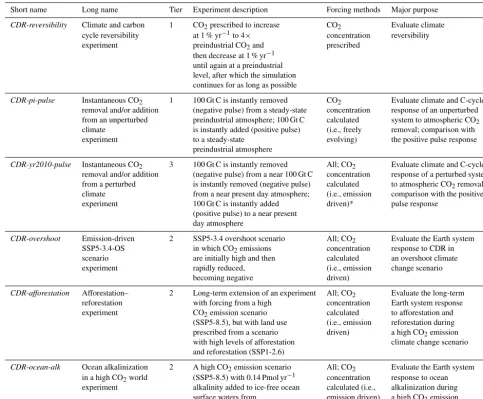
If CO2emissions are not reduced quickly enough and more warming occurs than is desirable or tolerable, then it is im-portant to understand if CDR has the potential to “reverse” climate change. Here we propose an idealized Tier 1 exper-iment that is designed to investigate CDR-induced climate “reversibility” (Fig. 1, Table 2). This experiment investigates the “reversibility” of the climate system by leveraging the prescribed 1 % yr−1CO2concentration increase experiment that was done for prior CMIPs and is a key run for CMIP6 (Eyring et al., 2016; Meehl et al., 2014). The CDRMIP exper-iment starts from the 1 % yr−1CO2 concentration increase experiment,1pctCO2, and then at the 4×CO2concentration level prescribes a −1 % yr−1 removal of CO2 from the at-mosphere to preindustrial levels (Fig. 1; this is also similar
Time (yr) A tmospheric C O2 (ppm) Preindustrial CDR-reversibility CMIP standard
experiment CDRMIP experiment 4 x preindustrial CO2
1% yr
-1 incr
ease 1% yr -1 decr ease Figure 2 Tem pera tur e A no m al y (°C) At m. t o O ce
an C fl
ux (Pg C y
r
-1)
Atmospheric CO2 (ppm) Experiment Year
4 x CO2
Return to inital CO2
UVic Mk3L-COAL
Increasin
g CO2
Decreasin g CO2
UVic Mk3L-COAL
0 200 400 600 800 1000 1200
a) b)
c) d)
Figure 1.Schematic of the CDRMIP climate and carbon cycle re-versibility experimental protocol (CDR-reversibility). From a prein-dustrial run at steady state atmospheric CO2 is prescribed to
in-crease and then dein-crease over a∼280-year period, after which it is held constant for as long as computationally possible.
to experiments in Boucher et al., 2012, and Zickfeld et al., 2016). This approach is analogous to an unspecified CDR application or DAC, in which CO2is removed to permanent storage to return atmospheric CO2to a prescribed level, i.e., a preindustrial concentration. To do this, CDR would have to counter emissions (unless they have ceased) and changes in atmospheric CO2 due to the response of the ocean and terrestrial biosphere. We realize that the technical ability of CDR methods to remove such enormous quantities of CO2 on such a relatively short timescale (i.e., in a few centuries) is unrealistic. However, branching from the existing CMIP
1pctCO2 experiment provides a relatively straightforward opportunity, with a high signal-to-noise ratio, to explore the effect of large-scale removal of CO2 from the atmosphere and issues involving reversibility (Fig. 2 shows exemplary
CDR-reversibilityresults from two models). 4.1.1 Protocol forCDR-reversibility
Prerequisite simulations. Perform the CMIP piControl
1142 D. P. Keller et al.: The Carbon Dioxide Removal Model Intercomparison Project (CDRMIP)
Table 2.Climate and carbon cycle reversibility experiment (CDR-reversibility) simulations. All simulations are required to complete the experiment.
CMIP6 Experiment Simulation description Owning MIP Run length Initialized using
ID (years) a restart from
piControl Preindustrial prescribed CO2control simulation CMIP6 DECK 100a the model spin-up
1pctCO2 Prescribed 1 % yr−1CO2increase CMIP6 DECK 140b piControl
to 4×the preindustrial level CMIP6 DECK 140b piControl
1pctCO2-cdr 1 % yr−1CO2decrease from 4×the CDRMIP 200 min. 1pctCO2
preindustrial level until the preindustrial CO2 5000 max.
level is reached and held for as long as possible
aThis CMIP6 DECK should have been run for at least 500 years. Only the last 100 years are needed as a control forCDR-reversibility.bThis CMIP6 DECK
experiment is 150 years long. A restart forCDR-reversibilityshould be generated after 139 years when CO2is 4 times that ofpiControl.
Time (yr)
A
tmospheric C
O2
(ppm)
Pre-industrial
CDR-reversibility
CMIP Standard
Experiment
CDRMIP Experiment
4 x pre-industrial CO2
1% yr -1 incr
ease
1% yr
-1
decr ease
Figure 1
Te
m
pe
ra
tu
re
an
om
al
y (
°C
)
At
m
. t
o
oc
ea
n
C
flu
x
(P
g
C
yr
-1)
Atmospheric CO2 (ppm) Experiment year
4 x CO2
Return to inital CO2
UVic Mk3L-COAL
Increasin g CO2
Decreasin
g CO2
UVic Mk3L-COAL
0 200 400 600 800 1000 1200
(a) (b)
(c) (d)
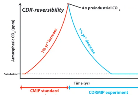
Figure 2. Exemplary climate and carbon cycle reversibility experiment (CDR-reversibility) results with the Mk3L-COAL Earth system model and the University of Victoria (UVic) Earth system model of intermediate complexity (models are described in Appendix D). The left panels show annual global mean(a)temperature anomalies (◦C; relative to pre-industrial temperatures) and(c)the atmosphere to ocean carbon fluxes (Pg C yr−1) versus the atmospheric CO2(ppm) during the first 280 years of the experiment (i.e., when CO2is increasing and decreasing). The right panels show the same(b)temperature anomalies and(d)the atmosphere to ocean carbon fluxes versus time. Note that the Mk3L-COAL simulation was only 400 years long.
may provide a link to them if they are already on the Earth System Grid Federation (ESGF) that hosts CMIP data.
The 1pctCO2-cdr simulation. Use the 4×CO2 restart from 1pctCO2 and prescribe a 1 % yr−1 removal of CO2 from the atmosphere (start removal at the beginning of the 140th year: 1 January) until the CO2 concentration reaches 284.7 ppm (140 years of removal). As in 1pctCO2the only externally imposed forcing should be the change in CO2(all other forcing is kept at that of year 1850). The CO2 concen-tration should then be held at 284.7 ppm for as long as
4.2 Direct CO2air capture with permanent storage
experiments (CDR-pi-pulse,CDR-year2010-pulse,
CDR-overshoot)
The idea of directly removing excess CO2 from the atmo-sphere (i.e., concentrations above preindustrial levels) and permanently storing it in some reservoir, such as a geolog-ical formation, is appealing because such an action would theoretically address the main cause of climate change: an-thropogenically emitted CO2that remains in the atmosphere. Laboratory studies and small-scale pilot plants have demon-strated that atmospheric CO2can be captured by several dif-ferent methods that are often collectively referred to as di-rect air capture (DAC) technology (Holmes and Keith, 2012; Lackner et al., 2012; Sanz-Pérez et al., 2016). Technology has also been developed that can place captured carbon in permanent reservoirs, i.e., carbon capture and storage (CCS) methods (Matter et al., 2016; Scott et al., 2013, 2015). DAC technology is currently prohibitively expensive to deploy on large scales and may be technically difficult to scale up (Na-tional Research Council, 2015), but it does appear to be a po-tentially viable CDR option. However, aside from the tech-nical questions involved in developing and deploying such technology, there remain questions about how the Earth sys-tem would respond if CO2 were removed from the atmo-sphere.
Here we propose a set of experiments that are designed to investigate and quantify the response of the Earth system to idealized large-scale DAC. In all experiments, atmospheric CO2 is allowed to freely evolve to investigate carbon cycle and climate feedbacks in response to DAC. The first two ide-alized experiments described below use the approach of an instantaneous (pulse) CO2removal from the atmosphere for this investigation. Instantaneous CO2removal perturbations were chosen since pulsed CO2addition experiments have al-ready been proven useful for diagnosing carbon cycle and cli-mate feedbacks in response to CO2perturbations. For exam-ple, previous positive CO2pulse experiments have been used to calculate global warming potential (GWP) and global tem-perature change potential (GTP) metrics (Joos et al., 2013). The experiments described below build upon the previous positive CO2pulse experiments, i.e., the PD100 and PI100 impulse experiments described in Joos et al. (2013), in which 100 Gt C is instantly added to preindustrial and near present day simulated climates. However, our experiments also pre-scribe a negative CDR pulse as opposed to just adding CO2 to the atmosphere. Two experiments are desirable because the Earth system response to CO2removal will be different when starting from an equilibrium state versus starting from a perturbed state (Zickfeld et al., 2016). One particular goal of these experiments is to estimate a global cooling poten-tial (GCP) metric based on a CDR impulse response func-tion (IRFCDR). Such a metric will be useful for calculating how much CO2is removed by DAC and how much DAC is needed to achieve a particular climate target.
The third experiment, which focuses on “negative emis-sions”, is based on the Shared Socioeconomic Pathway (SSP) 5-3.4 overshoot scenario and its long-term extension (Kriegler et al., 2016; O’Neill et al., 2016). This scenario is of interest to CDRMIP because after an initially high level of emissions, which follows the SSP5-8.5 unmitigated baseline scenario until 2040, CO2 emissions are rapidly re-duced with net CO2 emissions becoming negative after the year 2070 and continuing to be so until the year 2190 when they reach zero. In the original SSP5-3.4-OS scenario, the negative emissions are achieved using BECCS. However, as stated earlier there is currently no practical way to design a good multi-model BECCS experiment. Therefore, in our experiments negative emissions are achieved by simply re-moving CO2 from the atmosphere and assuming that it is permanently stored in a geological reservoir. While this may violate the economic assumptions underlying the scenario, it still provides an opportunity to explore the response of the climate and carbon cycle to potentially achievable levels of negative emissions.
According to calculations done with a simple climate model, MAGICC version 6.8.01 BETA (Meinshausen et al., 2011; O’Neill et al., 2016), the SSP5-3.4-OS scenario con-siderably overshoots the 3.4 W m−2 forcing level, with a peak global mean temperature of about 2.4◦C, before re-turning to 3.4 W m−2 at the end of the century. Eventually in the long-term extension of this scenario, the forcing sta-bilizes just above 2 W m−2, with a global mean temperature that should equilibrate at about 1.25◦C above preindustrial temperatures. Thus, in addition to allowing for an investi-gation into the response of the climate and carbon cycle to negative emissions, this scenario also provides the opportu-nity to investigate issues of reversibility, albeit on a shorter timescale and with less of an “overshoot” than in experiment
CDR-reversibility.
4.2.1 Instantaneous CO2removal and addition from an
unperturbed climate experimental protocol (CDR-pi-pulse)
This idealized Tier 1 experiment is designed to investigate how the Earth system responds to DAC when perturbed from an equilibrium state (Fig. 3, Table 3). The idea is to provide a baseline system response that can later be com-pared to the response of a perturbed system, i.e., experiment
1144 D. P. Keller et al.: The Carbon Dioxide Removal Model Intercomparison Project (CDRMIP)
CDRMIP experiment
CMIP standard experiment
CDR-pi-pulse
A
tmospheric C
O2
(ppm)
Time (yr) 200
225 250 275 300
325 Preindustrial spin-up run (fixed CO2)
100 Gt C removal run
Atmospheric CO2 allowed to
freely evolve 350
375
100 Gt C addition run
Figure 3. Schematic of the CDRMIP instantaneous CO2removal and addition from an unperturbed climate experimental protocol
(CDR-pi-pulse). Models are spun up for as long as possible with
a prescribed preindustrial atmospheric CO2concentration. Then
at-mospheric CO2is allowed to freely evolve for at least 100 years as a
control run. The negative–positive pulse experiments are conducted by instantly removing or adding 100 Gt C to the atmosphere of a simulation in which the atmosphere is at steady state and CO2can
freely evolve. These runs continue for as long as computationally possible.
Prerequisite simulation. This is a control simulation un-der preindustrial conditions with freely evolving CO2. All boundary conditions (solar forcing, land use, etc.) are ex-pected to remain constant. This is also the CMIP5 esmCon-trol simulation (Taylor et al., 2012) and the CMIP6 esm-piControl simulation (Eyring et al., 2016). Note that this is exactly the same as PI100 run 4 in Joos et al. (2013).
The esm-pi-cdr-pulse simulation.This is as inesm-Control
oresm-piControl, but with 100 Gt C instantaneously (within 1 time step) removed from the atmosphere in year 10. If models have CO2spatially distributed throughout the atmo-sphere, we suggest removing this amount in a uniform man-ner. After the negative pulse, ESMs should continue the run for at least 100 years, while EMICs and box models are en-couraged to continue the run for at least 1000 years (and up to 5000 years if possible). Figure 4 shows example esm-pi-cdr-pulsemodel responses.
The esm-pi-CO2pulse simulation.This is the same as esm-pi-cdr-pulse, but add a positive 100 Gt C pulse (within 1 time step) as in Joos et al. (2013) instead of a negative one. If models have CO2spatially distributed throughout the atmo-sphere, we suggest adding CO2 in a uniform manner. Note that this would be exactly the same as the PI100 run 5 in Joos et al. (2013) and can thus be compared to this earlier study.
At
m
os
ph
er
ic C
O2
(p
pm)
O
ce
an
to
at
m
. C
fl
ux
(P
g
C
yr
-1)
Time (years) after 100 Gt C removal (a)
(c) 285
La
nd
to
at
m
. C
fl
ux
(P
g
C
yr
-1) 275
265
255
245
235 (b)
0 100 200 300 400 500
Initial CO2 concentration
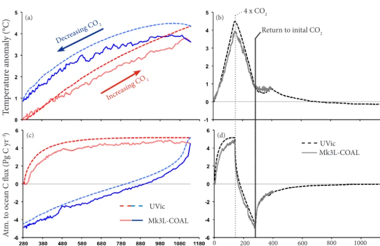
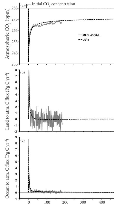
Figure 4.Exemplary instantaneous CO2removal from a
preindus-trial climate experiment (CDR-pi-pulse) results from the
esm-pi-cdr-pulsesimulation with the Mk3L-COAL Earth system model
and the University of Victoria (UVic) Earth system model of inter-mediate complexity (models are described in Appendix D).(a) At-mospheric CO2vs. time,(b)the land to atmosphere carbon flux vs.
time, and(c)the ocean to atmosphere carbon flux vs. time. Note that the Mk3LCOAL simulation was only 184 years long.
4.2.2 Instantaneous CO2removal from a perturbed
climate experimental protocol (CDR-yr2010-pulse)
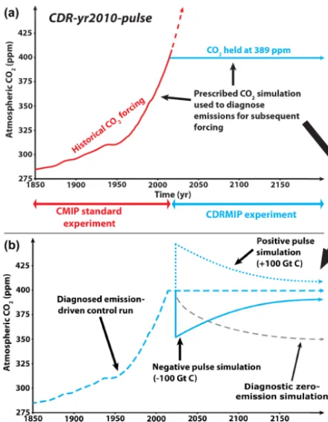
Figure 5. Schematic of the CDRMIP instantaneous CO2removal
and addition from a perturbed climate experimental protocol (
CDR-yr2010-pulse).(a)Initially historical CO2 forcing is prescribed and
then held constant at 389 ppm (∼year 2010) while CO2emissions are diagnosed.(b)A control simulation is conducted using the diag-nosed emissions. The negative–positive pulse experiments are con-ducted by instantly removing or adding 100 Gt C to the atmosphere of the CO2-emission-driven simulation 5 years after CO2reaches
389 ppm. Another control simulation is also conduced that sets emissions to zero at the time of the negative pulse. The emission-driven simulations continue for as long as computationally possible.
modeling research, for example CMIP, and may be able to use a “restart” file to initialize the first run, which should re-duce the effort needed to perform the complete experiment.
Prerequisite simulation.This is a prescribed CO2run. His-torical atmospheric CO2is prescribed until a concentration of 389 ppm is reached (∼year 2010; Fig. 5a). Other historical forcing, i.e., from CMIP, should also be applied. An exist-ing run or setup from CMIP5 or CMIP6 may also be used to reach a CO2concentration of 389 ppm, for example the RCP 8.5 CMIP5 simulation or the CMIP6historicalexperiment. During this run, compatible emissions should be frequently diagnosed (at least annually).
The yr2010CO2 simulation.Atmospheric CO2should be held constant at 389 ppm with other forcing, like land use and aerosol emissions, also held constant (Fig. 5a). ESMs should continue the run at 389 ppm for at least 105 years,
while EMICs and box models are encouraged to continue the run for as long as needed for the subsequent simulations (e.g., 1000+years). During this run, compatible emissions should be frequently diagnosed (at least annually). Note that when combined with the prerequisite simulation described above this is exactly the same as the PD100 run 1 in Joos et al. (2013).
The esm-yr2010CO2-control simulation. This is a diag-nosed emissions control run. The model is initialized from the preindustrial period (i.e., using a restart from either pi-Controloresm-piControl) with the emissions diagnosed in thehistoricalandyr2010CO2simulations, i.e., year 1850 to approximately year 2115 for ESMs and longer for EMICs and box models (up to 5000 years). All other forcing should be as in the historical and yr2010CO2 simulations. At-mospheric CO2 must be allowed to freely evolve. The re-sults should be quite close to those in the historical and
yr2010CO2simulations. If there are significant differences, for example due to climate–carbon cycle feedbacks that be-come evident when atmospheric CO2 is allowed to freely evolve, then they must be diagnosed and used to adjust the CO2emission forcing. In some cases it may be necessary to perform an ensemble of simulations to diagnose compatible emissions. Note that this is exactly the same as the PD100 run 2 in Joos et al. (2013). As in Joos et al. (2013), if computa-tional time is an issue and if a group is sure that CO2remains at a nearly constant value with the emissions diagnosed in
yr2010CO2, theesm-yr2010CO2-controlsimulation may be skipped. This may only apply to ESMs and it is strongly rec-ommended to perform theesm-yr2010CO2-control simula-tion to avoid model drift.
The esm-yr2010CO2-cdr-pulse simulation.This is a CO2 removal simulation. Setup is initially as in the esm-yr2010CO2-controlsimulation. However, a “negative” emis-sions pulse of 100 Gt C is subtracted instantaneously (within 1 time step) from the atmosphere 5 years after the time at which CO2was held constant in theesm-yr2010CO2-control simulation (this should be at the beginning of the year 2015), with the run continuing thereafter for at least 100 years (up to 5000 years if possible). If models have CO2spatially dis-tributed throughout the atmosphere, we suggest removing this amount in a uniform manner. It is crucial that the nega-tive pulse be subtracted from a constant background concen-tration of∼389 ppm. All forcing, including CO2emissions, must be exactly as in theesm-yr2010CO2-controlsimulation so that the only difference between these runs is that this one has had CO2instantaneously removed from the atmosphere.
The esm-yr2010CO2-noemit simulation. This is a zero CO2 emissions control run. Setup is initially as in the
esm-yr2010CO2-1146 D. P. Keller et al.: The Carbon Dioxide Removal Model Intercomparison Project (CDRMIP)
Table 3.Instantaneous CO2removal from an unperturbed climate experiment (CDR-pi-pulse) simulation. All simulations are required to
complete the experiment.
CMIP6 Experiment Simulation description Owning MIP Run length Initialized using
ID (years) a restart from
esm-piControl Preindustrial freely evolving CMIP6 DECK 100* the model
CO2control simulation spin-up
esm-pi-cdr-pulse 100 Gt C is instantly removed (negative pulse) CDRMIP 100 min. esm-piControl
from a preindustrial atmosphere 5000 max.
esm-pi-CO2pulse 100 Gt C is instantly added (positive pulse) CDRMIP 100 min. esm-piControl
to a preindustrial atmosphere 5000 max.
* This CMIP6 DECK should have been run for at least 500 years. Only the last 100 years are needed as a control forCDR-pi-pulse.
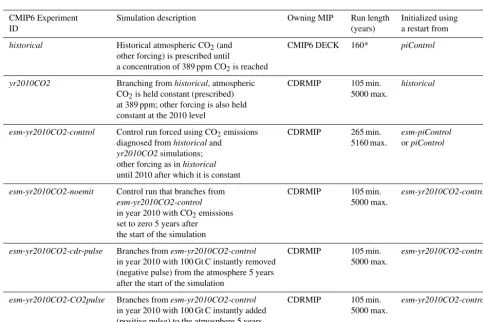
Table 4.Instantaneous CO2removal from a perturbed climate experiment (CDR-yr2010-pulse) simulation. All simulations are required to
complete the experiment.
CMIP6 Experiment Simulation description Owning MIP Run length Initialized using
ID (years) a restart from
historical Historical atmospheric CO2(and CMIP6 DECK 160* piControl
other forcing) is prescribed until
a concentration of 389 ppm CO2is reached
yr2010CO2 Branching fromhistorical, atmospheric CDRMIP 105 min. historical
CO2is held constant (prescribed) 5000 max.
at 389 ppm; other forcing is also held constant at the 2010 level
esm-yr2010CO2-control Control run forced using CO2emissions CDRMIP 265 min. esm-piControl
diagnosed fromhistoricaland 5160 max. orpiControl
yr2010CO2simulations;
other forcing as inhistorical
until 2010 after which it is constant
esm-yr2010CO2-noemit Control run that branches from CDRMIP 105 min. esm-yr2010CO2-control
esm-yr2010CO2-control 5000 max.
in year 2010 with CO2emissions
set to zero 5 years after the start of the simulation
esm-yr2010CO2-cdr-pulse Branches fromesm-yr2010CO2-control CDRMIP 105 min. esm-yr2010CO2-control
in year 2010 with 100 Gt C instantly removed 5000 max.
(negative pulse) from the atmosphere 5 years after the start of the simulation
esm-yr2010CO2-CO2pulse Branches fromesm-yr2010CO2-control CDRMIP 105 min. esm-yr2010CO2-control
in year 2010 with 100 Gt C instantly added 5000 max.
(positive pulse) to the atmosphere 5 years after the start of the simulation
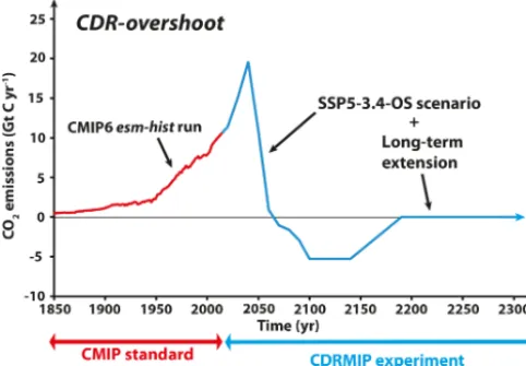
Figure 6.Schematic of the CDRMIP emission-driven SSP5-3.4-OS scenario experimental protocol (CDR-overshoot). A CO2 -emission-driven historical simulation is conducted until the year 2015. Then an emission-driven simulation with SSP5-3.4-OS scenario forcing is conducted. This simulation is extended until the year 2300 using SSP5-3.4-OS scenario long-term extension forcing. Thereafter, runs may continue for as long as computationally possible with constant forcing after the year 2300.
control simulation. This experiment will be used to iso-late the Earth system response to the negative emissions pulse in the esm-yr2010CO2-cdr-pulse simulation, which convolves the response to the negative emissions pulse with the lagged response to the preceding positive CO2 emis-sions (diagnosed with the zero emisemis-sions simulation). The response to the negative emissions pulse will be calculated as the difference betweenesm-yr2010CO2-cdr-pulseand esm-yr2010CO2-noemitsimulations.
The esm-yr2010CO2-CO2pulse simulation. This is a
CO2 addition simulation. Setup is initially as in the
esm-yr2010CO2-cdr-pulse simulation. However, a “positive” emissions pulse of 100 Gt C is added instantaneously (within 1 time step), with the run continuing thereafter for a mini-mum of 100 years. If models have CO2spatially distributed throughout the atmosphere, we suggest adding CO2 in a uniform manner. If possible, extend the runs for at least 1000 years (and up to 5000 years). It is crucial that the pos-itive pulse be added to a constant background concentration of∼389 ppm. All forcing, including CO2emissions, must be exactly as in theesm-yr2010CO2-controlsimulation so that the only difference between these runs is that this one has had CO2instantaneously added to the atmosphere. Note that this would be exactly the same as the PD100 run in Joos et al. (2013). This will be used to investigate if, after positive and negative pulses, carbon cycle and climate feedback re-sponses, which are expected to be opposite in sign, differ in magnitude and temporal scale. The results can also be com-pared to Joos et al. (2013).
4.2.3 Emission-driven SSP5-3.4-OS experimental protocol (CDR-overshoot)
This Tier 2 experiment explores CDR in an “overshoot” cli-mate change scenario, the SSP5-3.4-OS scenario (Fig. 6, Ta-ble 5). To start, groups must perform the CMIP6 emission-driven historical simulation, esm-hist. Then using this as a starting point, conduct an emissions-driven SSP5-3.4-OS scenario simulation, esm-ssp534-over (starting on 1 Jan-uary 2015), that includes the long-term extension to the year 2300. All non-CO2forcing should be identical to that in the ScenarioMIPssp534-overandssp534-over-extsimulations. If computational resources are sufficient, we recommend that theesm-ssp534-oversimulation be continued for at least an-other 1000 years with year 2300 forcing; i.e., the forcing is held constant at year 2300 levels as the simulation continues for as long as possible (up to 5000 years) to better understand processes that are slow to equilibrate, for example ocean car-bon and heat exchange or permafrost dynamics.
4.3 Afforestation–reforestation experiment (CDR-afforestation)
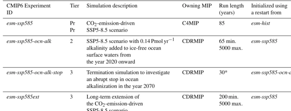
Enhancing the terrestrial carbon sink by restoring or extend-ing forest cover, i.e., reforestation and afforestation, has of-ten been suggested as a poof-tential CDR option (National Re-search Council, 2015; The Royal Society, 2009). Enhancing this sink is appealing because terrestrial ecosystems have cu-mulatively absorbed over one-quarter of all fossil fuel emis-sions (Le Quéré et al., 2016) and could potentially sequester much more. Most of the key questions concerning land use change are being addressed by LUMIP (Lawrence et al., 2016). These include investigations into the potential and side effects of afforestation and reforestation to mitigate cli-mate change, for which they have designed four experiments (LUMIP Phase 2 experiments). However, three of these ex-periments are CO2concentration driven and thus are unable to fully investigate the climate–carbon cycle feedbacks that are important for CDRMIP. The LUMIP experiment in which CO2 emissions force the simulation,esm-ssp585-ssp126Lu, will allow for climate–carbon cycle feedbacks to be investi-gated. Unfortunately, since this experiment ends in the year 2100 it is too short to answer some of the key CDRMIP ques-tions (Sect. 1.2). We have therefore decided to extend this LUMIP experiment within the CDRMIP framework as a Tier 2 experiment (Table 6) to better investigate the longer-term CDR potential and risks of afforestation and reforestation.
1148 D. P. Keller et al.: The Carbon Dioxide Removal Model Intercomparison Project (CDRMIP)
Table 5.Emission-driven SSP5-3.5-OS scenario experiment (CDR-overshoot) simulations. All simulations are required to complete the experiment.
CMIP6 Experiment Simulation description Owning Run length Initialized using
ID MIP (years) a restart from
esm-hist Historical simulation forced CMIP6 DECK 265 esm-piControl
with CO2emissions orpiControl
esm-ssp534-over CO2-emission-driven SSP5-3.4 CDRMIP 85 min. esm-hist
overshoot scenario simulation 5000 max.
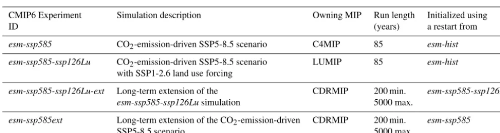
Table 6.Afforestation–reforestation experiment (CDR-afforestation) simulations. All simulations are required to complete the experiment.
CMIP6 Experiment Simulation description Owning MIP Run length Initialized using
ID (years) a restart from
esm-ssp585 CO2-emission-driven SSP5-8.5 scenario C4MIP 85 esm-hist
esm-ssp585-ssp126Lu CO2-emission-driven SSP5-8.5 scenario LUMIP 85 esm-hist
with SSP1-2.6 land use forcing
esm-ssp585-ssp126Lu-ext Long-term extension of the CDRMIP 200 min. esm-ssp585-ssp126Lu
esm-ssp585-ssp126Lusimulation 5000 max.
esm-ssp585ext Long-term extension of the CO2-emission-driven CDRMIP 200 min. esm-ssp585
SSP5-8.5 scenario 5000 max.
reforestation scenario in a high CO2world. This is similar to the approach of Sonntag et al. (2016) using RCP 8.5 emis-sions combined with prescribed RCP 4.5 land use.
4.3.1 CDR-afforestationexperimental protocol
Prerequisite simulations. Conduct the C4MIP emission-driven esm-ssp585 simulation, which is a control run, and the LUMIP Phase 2 experiment esm-ssp585-ssp126Lu
(Lawrence et al., 2016). Generate restart files in the year 2100.
The esm-ssp585-ssp126Lu-ext simulation.Using the year 2100 restart from the esm-ssp585-ssp126Lu experiment, it continues the run with the same LUMIP protocol (i.e., an emission-driven SSP5-8.5 simulation with SSP1-2.6 land use instead of SSP5-8.5 land use) until the year 2300 using the SSP5-8.5 and SSP1-2.6 long-term extension data (O’Neill et al., 2016). If computational resources are sufficient, we rec-ommend that the simulation be continued for at least another 1000 years with year 2300 forcing (i.e., forcing is held at year 2300 levels as the simulation continues for as long as possible; up to 5000 years). This is to better understand pro-cesses that are slow to equilibrate, for example ocean carbon and heat exchange or permafrost dynamics, and the issue of permanence.
The esm-ssp585ext simulation. The emission-driven esmSSP5-8.5 simulation must be extended beyond the year 2100 to serve as a control run for the esm-ssp585-ssp126Lu-ext simulation. This will require using the ScenarioMIP
ssp585-extforcing, but driving the model with CO2 emis-sions instead of prescribing the CO2concentration. If com-putational resources are sufficient, the simulation should be extended even further than in the official SSP scenario, which ends in year 2300, by keeping forcing constant after this time (i.e., forcing is held at year 2300 levels as the simulation con-tinues for as long as possible; up to 5000 years).