Classification complexity in myoelectric pattern recognition

(1)

R E S E A R C H

Open Access

Classification complexity in myoelectric

pattern recognition

Niclas Nilsson

1*

, Bo Håkansson

1

and Max Ortiz-Catalan

1,2

Abstract

Background:Limb prosthetics, exoskeletons, and neurorehabilitation devices can be intuitively controlled using

myoelectric pattern recognition (MPR) to decode the subject’s intended movement. In conventional MPR, descriptive electromyography (EMG) features representing the intended movement are fed into a classification algorithm. The separability of the different movements in the feature space significantly affects the classification complexity. Classification complexity estimating algorithms (CCEAs) were studied in this work in order to improve feature selection, predict MPR performance, and inform on faulty data acquisition.

Methods:CCEAs such as nearest neighbor separability (NNS), purity, repeatability index (RI), and separability index

(SI) were evaluated based on their correlation with classification accuracy, as well as on their suitability to produce highly performing EMG feature sets. SI was evaluated using Mahalanobis distance, Bhattacharyya distance, Hellinger distance, Kullback–Leibler divergence, and a modified version of Mahalanobis distance. Three commonly used classifiers in MPR were used to compute classification accuracy (linear discriminant analysis (LDA), multi-layer perceptron (MLP), and support vector machine (SVM)). The algorithms and analytic graphical user interfaces produced in this work are freely available in BioPatRec.

Results:NNS and SI were found to be highly correlated with classification accuracy (correlations up to 0.98 for both

algorithms) and capable of yielding highly descriptive feature sets. Additionally, the experiments revealed how the level of correlation between the inputs of the classifiers influences classification accuracy, and emphasizes the classifiers’sensitivity to such redundancy.

Conclusions:This study deepens the understanding of the classification complexity in prediction of motor volition

based on myoelectric information. It also provides researchers with tools to analyze myoelectric recordings in order to improve classification performance.

Keywords:Classification complexity, Myoelectric pattern recognition, Electromyography, Prosthesis control

Background

Decoding of motor volition via myoelectric pattern rec-ognition (MPR) has many clinical applications such as prosthetic control [1], phantom limb pain treatment [2], and rehabilitation after stroke [3]. Research on MPR has focused on classifiers [4], pre-processing algorithms [5], and electromyography (EMG) acquisition [6], among other factors that influence the classification outcome. Reaz et al. studied different attributes of EMG signals, such as signal-to-noise ratio, that decrease the complex-ity of MPR [7]. However, limited studies have been

conducted on the complexity of the classification task it-self. Information on complexity prior to classification can inform on specific conflicting classes and flawed data acquisition. Understanding of classification com-plexity can also be used to select optimal features and evaluate trade-offs between the amount of classes and their separability.

Most MPR algorithms use EMG features extracted from overlapping time windows as the classifier input. Therefore, the resulting classification accuracy is dependent on the features used to describe the EMG signals. The performance of a variety of such features, and feature selection algorithms, have been studied previously [8, 9]. Two feature selecting algorithms, * Correspondence:[email protected]

1_{Department of Electrical Engineering, Chalmers University of Technology,}

Gothenburg, Sweden

Full list of author information is available at the end of the article

(2)

namely minimum redundancy and maximum rele-vance [10], and Markov random fields [11], were ap-plied to an electrode array by Liu et al. [12], who used Kullback–Leibler divergence and feature scatter to rate the relevance and redundancy of features. The features were then ranked and selected into sets ac-cording to these ratings. Similarly, Bunderson et al. defined three data quality indices – namely, repeat-ability index (RI), mean semi-principal axis, and sep-arability index (SI) – to evaluate the changes in data

quality over repeated recordings of EMG [13].

Classification complexity estimation was not investi-gated in the aforementioned studies, but algorithms intended to quantify attributes relevant to the com-plexity of pattern recognition tasks were introduced.

Classification complexity has been studied outside the field of MPR. Singh suggested two nonparametric multiresolution complexity measures: nearest neighbor separability (NNS) and purity [14]. These complexity measures were compared with common statistical

similarity measures, such as Kullback–Leibler

divergence, Bhattacharyya distance, and Mahalanobis distance, and were found to yield a higher correlation

with classification accuracy. These classification

complexity estimating algorithms (CCEAs), along with Hellinger distance, were investigated in the present study with a focus on their relevance for MPR.

In the present study, CCEAs were evaluated based on their correlation with offline classification accuracy and real-time classification performance. Consequently, different attributes were revealed about the CCEAs, classification algorithms, and features descriptiveness. One such attributes–channel correlation dependency– was investigated further. The CCEAs that were found to yield high correlation with classification accuracy (NNS and SI) were then used for feature selection and

benchmarked against features sets found in the

literature.

The result of these experiments provided evidence of the suitability of CCEAs to predict MPR

perform-ance. The algorithms used in this work were

implemented and made freely available in BioPatRec, an open-source platform for development and bench-marking of algorithms used in advanced myoelectric control [15, 16].

Methods

Data sets

Two data sets were used in this study and both were recorded on healthy subjects. The first set contained

individual movements (IM data): 20 subjects, four

EMG channels, 14 bits Analog to Digital Conversion

(ADC), and 11 classes (hand open/close, wrist

flexion/extension, pro/supination, side grip, fine grip,

agree or thumb up, pointer or index extension, and rest or no movement) [15]. The second set contained

individual and simultaneous movements (SM data):

17 subjects, eight EMG channels, 16 bits ADC, and 27 classes (hand open/close, wrist flexion/extension, pro/supination, and all their possible combinations) [17]. Disposable Ag/AgCl (Ø = 1 cm) electrodes in a bipolar configuration (2 cm inter-electrode distance) were used in both sets. The bipoles were evenly spaced around the most proximal third of the forearm, with the first channel placed along the ex-tensor carpi ulnaris. Subjects were seated comfortably with their elbow flexed at 90 degrees and forearm supported, leaving only the hand to move freely. The data sets, along with details on demographics and acquisition hardware, are available online as part of BioPatRec [16]. Table 1 summarizes these data sets.

Signal acquisition, pre-processing and feature extraction

BioPatRec recording routines guided the subjects to perform each movement three times with resting periods in between. The instructed contraction time, as well as the resting time, was 3 s. The initial and final 15% of each contraction was discarded as this

normally corresponds to delayed response and

anticipatory relaxation by the subject, while the remaining central 70% still preserves portions of the dynamic contraction [15].

Time windows of 200 ms were extracted from the concatenated contraction data using 50 ms time increment. Features were then extracted from each time window and distributed in sets used for training (40%), validation (20%), and testing (40%) of the classifiers. The testing sets were never seen by the classifier during training or validation. A 10-fold cross-validation was performed by randomizing the feature vectors between the three sets before training and testing.

The following EMG signal features were used as implemented in BioPatRec [15, 16, 18]. In the time

domain: mean absolute value (tmabs), standard

deviation (tstd), variance (tvar), waveform length (twl), RMS (trms), zero-crossing (tzc), slope sign changes (tslpch), power (tpwr), difference abs. Mean (tdam), max fractal length (tmfl), fractal dimension Higuchi (tfdh), fractal dimension (tfd), cardinality

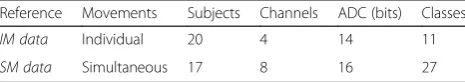
Table 1Summary of data sets

Reference Movements Subjects Channels ADC (bits) Classes

IM data Individual 20 4 14 11

SM data Simultaneous 17 8 16 27

(3)

(tcard), and rough entropy (tren). In the frequency domain: waveform length (fwl), mean (fmn) and me-dian (fmd). Feature vectors were constructed by sets of these features extracted from all channels, as com-monly done in MPR and implemented in BioPatRec (for a detailed explanation see reference [15]).

Classification complexity estimating algorithms

The classification complexity estimating algorithms (CCEAs) were designed to return classification complex-ity estimates (CCEs) for each movement separately ( indi-vidual result), and averaged over all movements (average results).Individual resultsprovide information that facil-itates the choice of movements to be included in a given MPR problem by distinguishing conflicting classes. Aver-age result considers the complete feature space, includ-ing all movements, and can therefore be used to evaluate and compare feature sets used to build the fea-ture space. The CCEAs used are outlined below.

Separability index

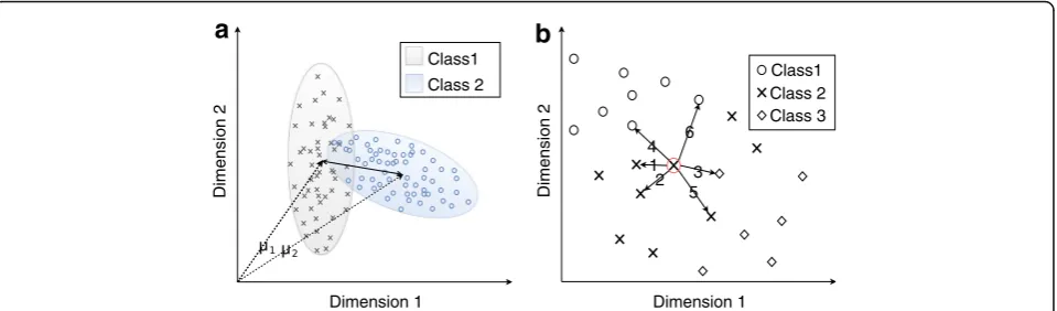
Separability index (SI) was implemented as introduced by Bunderson et al.; that is, the average of the distances between all movements and their most conflicting neighbor [13]. Figure 1a illustrates the distance and con-flict between two classes in an exemplary two-dimensional feature space.

The aforementioned distance was defined by Bunder-son et al. to be half the Mahalanobis distance, resulting in the following equation:

SI¼X

K

i¼1

min

j¼1;…;i−1;iþ1;…;K

1 2

ffiffiffiffiffiffiffiffiffiffiffiffiffiffiffiffiffiffiffiffiffiffiffiffiffiffiffiffiffiffiffiffiffiffiffiffiffiffiffiffiffiffi

μi−μj

T

S−_i1 μ_i−μ_j

r !

whereKis the number of classes or movements, andμx

and Sx are mean vectors and covariance matrices for classx,respectively.

This definition only considers the covariance of the target movement (Si), and not that of the comparing movement (that is, Sj). We considered this particular formulation as a potential limitation, so we introduced additional distance definitions. The distance definitions were used under the assumption of normality as Maha-lanobis distancewas defined under the same assumption [19]. The introduced distance definitions are described in Table 2.

Nearest neighbor Separability

Nearest neighbor separability (NNS) was inspired by the algorithm with the same name defined by Singh [14]. It is based on the dominance of nearest neighbors, in fea-ture space, belonging to the same class (movement) as a target data point. The contributions of the nearest neighbors are weighted by their proximity to the target point and the result is normalized to be a value between 0 and 1. Let

b pð t;piÞ ¼

1; 0;

if p_t;p_i∈C if p_t∈C;p_i∉C

Wherept.is the target point,piispt.:si-thnearest neigh-bor and C is a class. The aforementioned dominance is then defined as:

dt ¼ X

k

i¼1

1

i !−1_X_k

i¼1

b pð t;p_iÞ i

A target point and its six nearest neighbors are illus-trated in Fig. 1b.

The end result is the average dominance:

NNS¼ 1

N XN

i¼1

di

WhereNis the total number of samples.

Class1

1

2 3

6 4

5

b

Dimension 2

Dimension 1

Dimension 2

Dimension 1 Class1 Class 2

a

µ

Class 2 Class 3

µ

(4)

Table 2 Distance definitions for SI Distanc e defin ition D escription Maha lanobis dista nce Ma halan obis dist ance was design ed to me asure the dista nce betw een a distribu tion and a sing le point [ 19 ]. H alf the Mah alanob is dist ance wil l b e the valu e referred to as Mah alanob is dist ance here after becau se that is how it was originall y used in SI [ 13 ]. Ma halan obis dist ance for multivariate normal distr ibutio ns is de fined as:

DM 2

¼ 1 2 ffiffiffiffiffiffiffiffi ffiffiffiffiffiffiffiffiffiffiffiffiffiffiffiffiffiffiffiffiffiffiffiffiffiffiffiffiffiffi ffi μ1 − μ2 ðÞ T S − 1 1 μ1 − μ2 ðÞ q Bhatta char yya Distanc e Bha ttach aryya distance is a measuremen t o f statist ical simil arity betw een two distr ibutio ns bas ed on the Bha ttach aryya Coeffic ient (BC) [ 24 ]. Un like Mahalan obis dist ance , Bha ttach aryya distance takes both the dis tance and similarity in cova riance betwee n the distribu tions into account. In this study, the square ro ot of Bha ttachar yya dist ance was used to equat e the formulation of Ma halanob is dist ance an d faci litate com parison . Bha ttach aryya coefficient for the continu ous probability distr ibution s p an d q is defin ed as: BC ¼ R ffiffiffiffiffiffiffiffiffiffiffiffiffiffiffiffi ffi px ðÞ qx ðÞ p dx Bha ttach aryya distance as fun ction of Bhatta charyy a coeff icient: ffiffiffiffi ffi DB p ¼ ffiffiffiffiffiffi ffiffiffiffiffiffiffiffiffiffiffiffiffi ffi −

1ln2

BC ðÞ q Bha ttach aryya distance for mu ltivariate normal distributions (square ro ot) [ 25 ]: ffiffiffiffi ffi DB p ¼ ffiffiffiffiffiffi ffiffiffiffiffiffiffiffiffiffiffiffiffiffiffiffiffiffiffiffiffiffiffiffiffiffiffiffiffiffiffiffiffiffiffiffiffiffiffiffiffiffiffiffiffiffiffiffiffiffiffiffiffiffiffiffiffiffiffiffiffiffiffiffiffiffiffiffiffi ffi

1μ8

1 − μ2 ðÞ T S − 1μ 1 − μ2 ðÞ −

1ln2

detS ffiffiffiffiffiffiffiffiffiffiffiffiffiffiffi ffi det S1 det S2 p r Kullback – Lei bler divergenc e K ullback – Lei bler dive rg enc e is a w e ll-known statist ical simil arity measu re that is typically used to de term ine wh ether an obse rved distribu tion, Q , is a sam ple of a true distribu tion, P [ 26 ]. K ullback – Lei bler dive rg enc e for mult ivariate normal distr ibutio ns is de fined as [ 25 ]: DKL ¼ 1 2 tr S1 − 1S 2 ðÞ þ μ1 − μ2 ðÞ T S − 1 1 μ1 − μ2 ðÞ − k þ ln det S1 det S2 Helli nger dista nce Hell inger dist ance is rel ated to Bhatta charyy a distance as it is also based on the Bhatta charyy a coeff icient [ 27 ]. The square of the Hell inger dist ance was used in this study to avoid com plex numbe rs app earing where the ass umpt ion of normal ity fails , and this valu e is refe rred to here as the Hellinger dist ance . Hell inger dist ance as a fu nction of the Bha ttachary ya coeff icient is de fined as: D

2¼H

1 − BC Hell inger dist ance for multivariate nor mal distr ibution s: D

2¼H

1 − detS 1 ðÞ 1 4 detS 2 ðÞ 1 4 detS 1 ðÞ 1 2 exp −

1μ8

1 − μ2 ðÞ T S − 1μ 1 − μ2 ðÞ no Mod ified Maha lanobi s Thi s me asure of statistical similarity is equal to the aforem entione d Mah alanob is dist ance , exce pt that it take s into account the cova riance matrix o f b o th distr ibution s being compared. The algorithm is rel ated to Bha ttach aryya distance , but is only focused o n the dis tance be tween the distr ibutio ns. This CCEA is refe rred to here as modif ied Mahala nobis and is de fined for multivariate nor mal distr ibution s as:

DMM 2

(5)

Unless stated otherwise, the parameter kis set to 120, which is the maximum number of nearest neighbors from the same class for the data sets of this study.

Purity

Purity was computed by dividing the feature hyperspace into smaller hyper cuboids called cells [14]. The cells were rated individually and high dominance of one class in one cell meant high purity for that cell. The final purity of a data set was the average over all cells and dif-ferent cell resolutions.

Repeatability index

The repeatability index (RI) measures how much indi-vidual classes varies between different occurrences using Mahalanobis distance[13]. The three repetitions during the recording session were the occurrences that were evaluated. The end result is the average Mahalanobis distance between the first repetition and the following ones for all movements.

Classifiers and topologies

Three common classifiers for MPR were used in this study: linear discriminant analysis (LDA), multi-layer perceptron (MLP), and support vector machine (SVM). A quadratic kernel function was used for SVM. The classifiers were utilized as implemented in BioPatRec [15] (code available online [16]), where LDA and SVM were implemented using Matlab’s statistical toolbox.

MLP and SVM are inherently capable of simultaneous classification when provided with the feature vectors of mixed (simultaneous) outputs, hereafter referred as “MIX”output configurations; that is, there is one output for every individual movement and combinations of movements produce the corresponding mix of outputs to be turned on. LDA’s output is computed by majority voting, which means it cannot produce simultaneous classification by creating a mixed output. However, clas-sifiers like LDA can still be used for simultaneous classi-fication using the label power set strategy, where the classifier is constructed having the same number of out-puts as the total number of classes. This configuration is referred to here as“all movements as individual” (AMI). Ortiz-Catalan et al. showed that AMI could also favor classifiers capable of mixed outputs [17]; therefore, MLP and SVM were evaluated in both MIX and AMI configu-rations for simultaneous predictions. In addition, LDA was also used in the One-Vs-One topology (OVO), as this has been shown to improve classification accuracy for individual movements [17, 20].

Evaluation and comparison

In order to evaluate the correlation between Classification Complexity Estimates (CCEs) and classification accuracy,

all features were used individually to classify all move-ments from each subject in both data sets, which provided a wide range of classification accuracies and their related CCEs. Correlations were then calculated considering the classification of each movements individually (individual results), or the average over all movements (average results).

The CCEAs were further used to select one set of two, three, and four features. CCEs were calculated for all possible combinations of features and the three sets – one for every number of features– predicting the high-est accuracy were selected. The selected sets are referred hereafter as thebest setsand were obtained using theIM dataset.

Ortiz-Catalan et al. used a genetic algorithm to find optimal feature sets of two, three, and four features based on classification performance [8]. Their proposed sets of two and three features were used as benchmark-ing sets in this study, along with the commonly used four-feature set proposed by Hudgins et al. [21]. These sets are referred in this study asreference sets:

Ref 2F:tstd, trms [8]

Ref 3F:tstd, fwl, fmd [8]

Ref 4F:tmabs, twl, tslpch, tzc [21]

Thebestandreference setsof equal number of features were compared to each other based on the resulting classification accuracy, as given by the three different classifiers. Classification accuracy corresponds to offline computations unless otherwise stated. Real-time testing

was done using the Motion Tests as implemented in

BioPatRec [15, 22]. CCEAs’ proficiency at predicting real-time performance was evaluated by their correlation with the completion time obtained from motion tests, which is the time from the first prediction not equal to restuntil 20 correct predictions are achieved. Similar to offline computations, one prediction was the classifica-tion of one 200 ms time window, and new predicclassifica-tions were produced every 50 ms (time increment). The subject was instructed to hold the requested movement until 20 correct predictions were achieved. If the number of cor-rect predictions was less than 20 after 5 s, thecompletion timewas set to 5 s. The real-time results were obtained fromIM dataset and relatedMotion Tests [22].

Wilcoxon signed-rank test (p < = 0.05) was used to evaluate statistical significant differences. Correlations were calculated using Spearman’s rho, since there was no clear linearity in the dependencies between accuracy and CCE.

Results

Separability index (SI)

(6)

Table 3Correlations for the different distance definitions

Average result Individual results

LDA (AMI) Single/OVO

MLP AMI/MIX SVM AMI/MIX LDA (AMI) Single/OVO MLP AMI/MIX SVM AMI/MIX Data set

Mahalanobis 0.72/0.91 0.90/0.91 0.79/0.80 0.81/0.92 0.84/0.85 0.70/0.68 SM

0.78/0.88 0.86/NA 0.71/NA 0.85/0.91 0.80/NA 0.60/NA IM

Bhattacharyya 0.74/0.97 0.98/0.97 0.79/0.82 0.69/0.91 0.93/0.91 0.66/0.65 SM

0.83/0.96 0.96/NA 0.68/NA 0.79/0.89 0.94/NA 0.68/NA IM

Kullback–Leibler 0.60/0.88 0.93/0.90 0.65/0.70 0.54/0.76 0.84/0.82 0.63/0.60 SM

0.51/0.72 0.80/NA 0.32/NA 0.65/0.75 0.87/NA 0.65/NA IM

Hellinger 0.68/0.94 0.98/0.96 0.75/0.77 0.69/0.90 0.93/0.91 0.66/0.65 SM

0.80/0.95 0.97/NA 0.66/NA 0.79/0.89 0.94/NA 0.68/NA IM

Modified Mahalanobis 0.92/0.97 0.92/0.95 0.94/0.95 0.79/0.91 0.88/0.89 0.74/0.71 SM

0.93/0.94 0.87/NA 0.83/NA 0.85/0.90 0.86/NA 0.71/NA IM

Correlations under“individual results”were calculated using classification accuracies and SIs from every individual movement, subject and feature, while those

under“average result”were derived using the average SI and classification accuracy per subject and feature. Both methods provide one correlation, although

“individual results”use more data. Classifiers were configured using AMI or MIX. Classifiers were used in the conventional“single”topology, apart from LDA, which

was used in“single”and OVO. The highest correlation values per column are highlighted in bold. All correlations were found to be statistically significant at

p< 0.01. The MIX configuration is not applicable (NA) for individual movements since there is not mixed outputs

0 20 40 60 80 100

LDA

corr=0.78 corr=0.51 corr=0.83 corr=0.8 corr=0.93

0 20 40 60 80 100

LDA (OVO)

0 20 40 60 80 100

MLP

0 1 2 3

Mahalanobis 0

20 40 60 80 100

SVM

corr=0.71

0 200 400 600 800

Kullback Leibler

corr=0.32

0 0.5 1 1.5

Bhattacharyya

corr=0.68

0 0.5 1

Hellinger

corr=0.66

0 0.5 1 1.5 2

Modified Mahalanobis

corr=0.83

(7)

in Table 3, where the highest value for every classifier is highlighted. Figures 2 and 3 shows plots of average result for IM and SM data sets, respectively, with the most correlating distance definition highlighted for classifiers individually. Table 3, Figs. 2 and 3 indicates that the most adequate distance definitions vary with the classifier.

Mahalanobis distance

Mahalanobis distance was found as the distance defin-ition that most closely correlated with LDA in an OVO topology for individual resultsusingSM data. The cor-responding classification accuracy against SI is plotted in Fig. 4a.

Kullback–Leibler divergence

Kullback–Leibler divergence was not found to yield higher correlation than any otherdistance definitionfor any of the classifiers; however, it was found to correlate most closely with theaverage results of MLP using both topologies. This correlation is visualized in Figs. 2 and 3. Owing to its low correlation with classification accuracy,

Kullback–Leibler divergencewas not used in the reaming experiments.

Bhattacharyya distance

Bhattacharyya distance was the most correlating dis-tance definitionfor MLP in bothAMIandMIX configu-rations. Plots of classification accuracy for the two classifiers against SI based onBhattacharyya distanceis shown in insets B and C of Fig. 4. Individual resultsare

presented and IM dataand SM data are used for AMI

andMIXconfigurations, respectively.

Hellinger distance

Bhattacharyya distanceandHellinger distanceare highly related as they are both based on the Bhattacharyya Coefficient. Table 3 confirms their resemblance as the correlations related to the two distance definitions are very similar in all cases. Naturally, Hellinger distance and Bhattacharyya distance are the distance definitions that most closely correlate with MLP MIX and AMI for individual result,and with MLPAMI foraverage result.

MLP AMI classification accuracy is plotted against

0 50 100

LDA AMI corr=0.72 corr=0.6 corr=0.74 corr=0.68 corr=0.92

0 50 100

LDA AMI (OVO)

0 50 100

MLP AMI corr=0.9 corr=0.93 corr=0.98 corr=0.98 corr=0.92

0 50 100

MLP MIX corr=0.91 corr=0.9 corr=0.97 corr=0.96 corr=0.95

0 50 100

SVM AMI corr=0.79 corr=0.65 corr=0.79 corr=0.75 corr=0.94

0 5 10 15

Mahalanobis 0

50 100

SVM MIX corr=0.8

0 50 100 150 200

Kullback Leibler

corr=0.7

0 1 2

Bhattacharyya

corr=0.82

0 0.5 1

Hellinger

corr=0.77

0 0.5 1 1.5 2

corr=0.95

(8)

Hellinger distance based SI in Fig. 4e, where individual resultsusingIM datais represented.

Modified Mahalanobis was found as the distance defin-itionthat correlates most closely with average results of LDA and SVM classification accuracy for all topologies and configurations. The same is true for individual results, except for LDA in an OVO topology. Insets E

and F of Fig. 4 show LDA AMI and SVM MIX

classi-fication accuracy plotted against SI based on Modified Mahalanobis. Modified Mahalanobis was the version of Mahalanobis distance used in the remaining results

because of its overall higher correlation with classifi-cation accuracy.

Nearest neighbor separabillity (NNS)

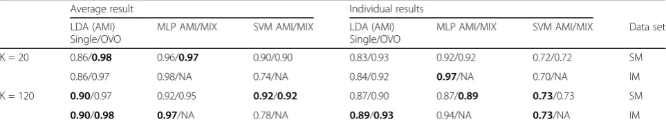
A summary of correlations with all classifiers for both data sets is presented in Table 4.

Table 4 also shows the influence of the parameter k. Figures 5 and 6 show plots of average resultfor the IM andSM data, respectively.

NNS is most correlated with LDA in an OVO top-ology, which is equivalent to the results obtained by SI based on Bhattacharyya distancefor the same classifier.

0 5 10 15

Mahalanobis 0

10 20 30 40 50 60 70 80 90 100

Accuracy

corr = 0.92

0 0.5 1 1.5 2 2.5

Bhattacharyya 0

10 20 30 40 50 60 70 80 90 100

Accuracy

corr = 0.94

0 0.5 1 1.5 2 2.5

Bhattacharyya 0

10 20 30 40 50 60 70 80 90 100

Accuracy

corr = 0.91

0 0.2 0.4 0.6 0.8 1

Hellinger 0

10 20 30 40 50 60 70 80 90 100

Accuracy

corr = 0.94

0 0.5 1 1.5 2 2.5 3

Mahalanobis Modified 0

10 20 30 40 50 60 70 80 90 100

Accuracy

corr = 0.79

0 0.5 1 1.5 2 2.5 3

Mahalanobis Modified 0

10 20 30 40 50 60 70 80 90 100

Accuracy

corr = 0.71 LDA AMI (OVO) and SM data MLP and IM data MLP MIX and SM data

MLP and IM data LDA AMI and SM data SVM MIX and SM data

Fig. 4Data distribution for the most correlating distance definitions. Plot matrix where the insets show classification accuracy plotted against the SI. One dot represents one movement, one subject, and one feature, which means that the number of dots is the number of movements multiplied by the number of subjects times the number of features. The plots represent the highlighted correlations in Table 3

Table 4Correlations between classification accuracy and nearest neighbor separability

MLP AMI/MIX SVM AMI/MIX LDA (AMI)

Single/OVO

MLP AMI/MIX SVM AMI/MIX Data set

K = 20 0.86/0.98 0.96/0.97 0.90/0.90 0.83/0.93 0.92/0.92 0.72/0.72 SM

0.86/0.97 0.98/NA 0.74/NA 0.84/0.92 0.97/NA 0.70/NA IM

K = 120 0.90/0.97 0.92/0.95 0.92/0.92 0.87/0.90 0.87/0.89 0.73/0.73 SM

0.90/0.98 0.97/NA 0.78/NA 0.89/0.93 0.94/NA 0.73/NA IM

(9)

0 0.2 0.4 0.6 0.8 1 NNS (k = 20)

0 20 40 60 80 100

Accuracy

LDA

corr=0.86

0 0.2 0.4 0.6 0.8 1

NNS (k = 20) LDA (OVO)

corr=0.97

0 0.2 0.4 0.6 0.8 1

NNS (k = 20) MLP

corr=0.98

0 0.2 0.4 0.6 0.8 1

NNS (k = 20) SVM

corr=0.74

0 0.2 0.4 0.6 0.8 1

NNS (k = 120) 0

20 40 60 80 100

Accuracy

corr=0.9

0 0.2 0.4 0.6 0.8 1

NNS (k = 120)

corr=0.98

0 0.2 0.4 0.6 0.8 1

NNS (k = 120)

corr=0.97

0 0.2 0.4 0.6 0.8 1

NNS (k = 120)

corr=0.78

Fig. 5The distribution of data from individual movement for NNS and all classifiers. Plot matrix where the insets shows classification accuracy plotted against NNS for the individual movements data set. One marker represents the average over all movements for one subject and one feature. Classifiers were used in the conventional“single”topology, apart from LDA, which was used in“single”and OVO. All correlations were found statistically significant atp< 0.01. The classifiers are grouped in columns and the results for different values of the parameter k are group in rows. The highest correlation values per column are highlighted by a thicker frame

0 0.5 1

NNS (k = 20) 0

20 40 60 80 100

Accuracy

LDA AMI

corr=0.86

0 0.5 1

NNS (k = 20) LDA AMI (OVO)

corr=0.98

0 0.5 1

NNS (k = 20) MLP AMI

corr=0.96

0 0.5 1

NNS (k = 20) MLP MIX

corr=0.97

0 0.5 1

NNS (k = 20) SVM AMI

corr=0.9

0 0.5 1

NNS (k = 20) SVM MIX

corr=0.9

0 0.5 1

NNS (k = 120) 0

20 40 60 80 100

Accuracy

corr=0.9

0 0.5 1

NNS (k = 120)

corr=0.97

0 0.5 1

NNS (k = 120)

corr=0.92

0 0.5 1

NNS (k = 120)

corr=0.95

0 0.5 1

NNS (k = 120)

corr=0.92

0 0.5 1

NNS (k = 120)

corr=0.92

Fig. 6The distribution of data from simultaneous movement for NNS and all classifiers. Plot matrix where the insets shows classification accuracy plotted against NNS for the simultaneous movements data set. One marker represents the average over all movements for one subject and one feature. Classifiers were configured using AMI or MIX. Classifiers were used in the conventional“single”topology, aside of LDA which was used in

(10)

The individual results for LDA using OVO are plotted for both data sets in Fig. 7.

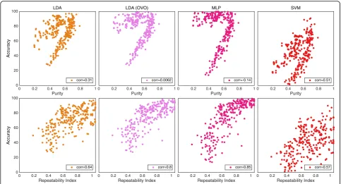
Purity and repeatability index

Purity and repeatability index resulted in low correlation with classification accuracy for all classifiers. The corre-lations for IM data can be found in Table 5. Figure 8

shows Individual results of MLP for the two

algo-rithms and the aforementioned data set. Because of the low correlation, purity was excluded from the

fol-lowing experiments, and RI from the Feature Sets

experiment.

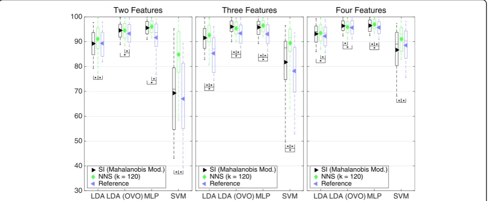
Feature sets

In this section, the best sets are compared with each other and thereference sets.In Fig. 9, thebest sets corre-sponding to the distance definitionsof SI are compared. The modified Mahalanobis sets are significantly higher than the otherdistance definitionssets in eight out of 12 cases, and averagely higher in all but the case where MLP is used with sets of three features. In that case,

Bhattacharyya distance andHellinger distance sets per-forming higher average classification accuracy.

The influence of parameter k of the NNS algorithm is shown in Fig. 10 by comparing thebest setsfor k = 120 and k = 20. The higher value of k leads to higher average classification accuracy in all cases. However, it is statisti-cally significant for SVM and three features only.

The members with the highest average classification accuracy were selected from Figs. 9 and 10 – modified Mahalanobis and k = 120, respectively – to be compared with the reference sets in Fig. 11. The NNS sets leads to significantly higher classification accuracy than the reference in all but one case, while modified Mahalanobis is significantly higher for nine out of 12. The average classification accuracy for the NNS sets is higher than modified Mahalanobis for all classifiers

except LDA in an OVO topology, where Modified

Mahalanobisis consistently higher.

Real time

Figure 12 summarizes the correlations between the mo-tion testresult completion timeand CCEs corresponding

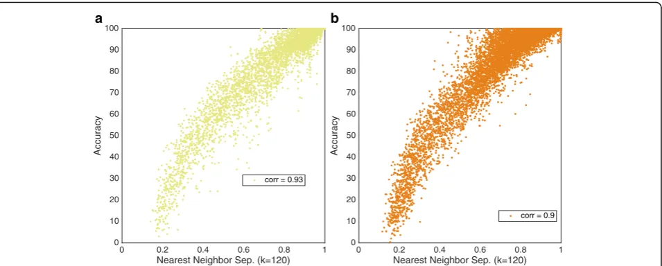
0 0.2 0.4 0.6 0.8 1

Nearest Neighbor Sep. (k=120) 0

10 20 30 40 50 60 70 80 90 100

Accuracy

corr = 0.93

0 0.2 0.4 0.6 0.8 1

Nearest Neighbor Sep. (k=120) 0

10 20 30 40 50 60 70 80 90 100

Accuracy

corr = 0.9

a b

Fig. 7Highest correlation for NNS. LDA (OVO) classification accuracy plotted against NNS for individual result. One dot represents one movements, one subject and one feature, meaning that the number of dots is the number of movements multiplied by the number of subjects multiplied by the number of features. The plots illustrate the highest correlation from Table 4.aLDA (OVO) and IM data.bLDA AMI (OVO) and SM data

Table 5Correlation for purity and repeatability index regarding classification accuracy

MLP AMI SVM AMI LDA (AMI)

Single/OVO

MLP AMI SVM AMI Data set

Purity 0.31/0.0062 ₋0.14 0.51 0.3/0.15 0.14 0.54 IM

Repeatability 0.64/0.8 0.85 0.57 0.23/0.36 0.45 0.16 IM

(11)

0 0.2 0.4 0.6 0.8 1 Purity

0 20 40 60 80 100

Accuracy

LDA

corr=0.31

0 0.2 0.4 0.6 0.8 1

Purity LDA (OVO)

corr=0.0062

0 0.2 0.4 0.6 0.8 1

Purity MLP

corr=-0.14

0 0.2 0.4 0.6 0.8 1

Purity SVM

corr=0.51

0 0.2 0.4 0.6 0.8 1

Repeatability Index 0

20 40 60 80 100

Accuracy

corr=0.64

0 0.2 0.4 0.6 0.8 1

Repeatability Index

corr=0.8

0 0.2 0.4 0.6 0.8 1

Repeatability Index

corr=0.85

0 0.2 0.4 0.6 0.8 1

Repeatability Index

corr=0.57

Fig. 8The distribution of data from individual movement for all classifiers with purity and repeatability. Plot matrix where the insets shows classification accuracy plotted against purity for row 1 and repeatability for row 2. The result is for the individual movements data set. One marker represents the average over all movements for one subject and one feature. Classifiers were used in the conventional“single”topology, apart from LDA, which was used in“single”and OVO. The classifiers are grouped in columns

LDA LDA (OVO) MLP SVM 30

40 50 60 70 80 90

100 Two Features

Modified Mahalanobis Bhattacharyya Hellinger

LDA LDA (OVO) MLP SVM

Three Features

Four Features

Fig. 9Classification accuracy for the best sets corresponding to distance definitions of SI. Boxplot of average classification accuracy over all movements when using the best sets representing the distance definitions found in the legends. The middle line of the box is the median, the marker is the mean, and the box extends to the 25th and the 75th percentiles for the bottom and the top, respectively. The different insets compare sets of different number of features. The result is derived from the IM data set. Classifiers were used in the conventional“single”topology, apart from LDA, which was used in

(12)

to RI, NNS, and SI based onmodified Mahalanobisand Bhattacharyya distance. Statistically significant correla-tions (p< 0.001) are highlighted by a darker frame.

Feature attribute

As the correlations used to evaluate the CCEAs were derived by use of one feature at a time, attributes of

features individually were revealed. Examples of such attributes are average classification accuracy and clas-sification accuracy variance. These two attributes are illustrated in Figs. 13 and 14 for IM and SM data, spectively. Figure 13 shows the five features that re-sulted in the highest and lowest average classification accuracy for classifiers separately.

40 50 60 70 80 90

100 Two Features

k = 20 k = 120

Three Features

k = 20 k = 120

Four Features

k = 20 k = 120

Fig. 10Classification accuracy for the best sets corresponding to distance definitions of the SI. Boxplot of average classification accuracy over all movements when using the best sets representing the distance definitions found in the legends. The middle line of the box is the median, the marker is the mean, and the box extends to the 25th and 75th percentiles for the bottom and the top, respectively. The different insets compare sets of different number of features. The result is derived from the IM data set. Classifiers were used in the conventional“single”topology, apart from LDA, which was used in“single”and OVO

40 50 60 70 80 90

100 Two Features

SI (Mahalanobis Mod.) NNS (k = 120) Reference

Three Features

Four Features

(13)

One attribute that was observed to highly influence the CCEAs’correlation with classification accuracy was channel correlation; that is, correlation between feature sequences extracted from the channels separately using only the feature considered. To illustrate this attribute,

average determinants of the channel correlation matrices over all subjects for the different features were extracted fromSM dataand shown in the bar diagram in Fig. 15.

The features marked by red color have low average cor-relation matrix determinants, which means a high 1.5

2 2.5 3 3.5 4 4.5 5

MLP - Completion Time

corr = -0.52 corr = -0.53

corr = -0.013

corr = -0.44

0.5 1 1.5 2 2.5 3 3.5

SI (Modified Mahalanobis) 1.5

2 2.5 3 3.5 4 4.5 5

LDA - Completion Time

corr = -0.54

1 1.5 2 2.5 3

SI (Bhattacharyya)

corr = -0.45

1 1.5 2 2.5

Repeatability Index

corr = 0.018

0.5 0.6 0.7 0.8 0.9

Nearest Neighbor Sep.

corr = -0.47

Fig. 12Real-time correlation for Classification Complexity Estimations. Plot matrix where the insets are completion time plotted against classification complexity estimates. Significant correlation (p< 0.001) is highlighted with bold frame

0 20 40 60 80 100

Accuracy

tcard tstd twl fwl trms tpwr tren fmd tfdh tfd

tstd trms twl tcard tmabs fmn tren fmd tfdh tfd

0 1 2 3 4 5

Separability Index

0 20 40 60 80 100

Accuracy

tcard tstd trms twl fwl fmn tren fmd tfdh tfd

0 1 2 3 4 5

Separability Index

tcard tstd trms tzc fwl tpwr tvar fmd tfdh tfd A

D

L MLP

) O V O ( A D

L SVM

(14)

correlation between channels, while the blue color repre-sents features of low channel correlation. Figure 16 shows how the two groups of features, red and blue from Fig. 15, cluster differently in classification accuracy against CCE plots.

The blue group has similar dependency on classifica-tion accuracy for the three classifiers, while the red clearly varies between them.

Discussion

Offline results Separability index

Modified Mahalanobis was the distance definition that had the greatest correlation with classification accuracy (Table 3). However, the distance definitions based on Bhattacharyya coefficient, being Bhattacharyya distance and Hellinger distance, had a higher correlation with 0

20 40 60 80 100

Accuracy

tstd tcard twl trms tren tpwr tvar fmd tfdh tfd

twl tstd trms tmabs tvar tzc fmn fmd tfdh tfd

0 1 2 3 4 5

Separability Index

0 20 40 60 80 100

Accuracy

tstd twl trms tmabs fwl tslpch fmn fmd tfdh tfd

0 1 2 3 4 5

Separability Index

tstd twl trms tmabs tcard tpwr tvar fmd tfdh tfd A

D

L MLP

) O V O ( A D

L SVM

Fig. 14High- and low-performing feature algorithms for the simultaneous movements data.Ellipses representing clusters for features in a classification accuracy against SI plots for results using the simultaneous movements data set. The SI distance definition is modified Mahalanobis. The ellipses are centered around the means of the feature clusters and constructed according to the covariance matrix. Every inset includes the feature algorithms with the top five and bottom five average classification accuracies for the classifier stated in the plot. The ellipses are coded by

redandbluecolor for low and high average classification accuracy, respectively. Classifiers were used in the conventional“single”topology, apart from LDA, which was used in“single”and OVO

tmabs tstd tvar twl trms tzc _{tslpch tpwr tdam tmfl tfdh tfd} tca

rd tre

n fwl fmn fmd

0 0.05 0.1 0.15 0.2 0.25 0.3 0.35

Mean Correlation Matrix Determinant

(15)

MLP’s classification accuracy. The Feature Attributes section shows that Bhattacharyya distancecompensates for the change in dependency to MLP classification ac-curacy caused by input correlation that is found in the other CCEAs. It should therefore be a more adequate distance definition for estimation of MLP classification complexity. However, as features are combined into sets, the feature correlation tend to decrease as larger feature vectors are formed using multiple features. This is prob-ably a reason for the absence of significantly higher clas-sification accuracy forBhattacharyya distance(Fig. 9).

Nearest neighbor separability

NNS has high correlation with classification accuracy for all classifiers, as shown in Table 4. Figure 10

shows that the best sets corresponding to NNS

per-form higher overall classification accuracy then both the SI best sets and the reference sets. The greatest benefit of NNS is that it does not assume normality of the distribution, which makes it more general. However, there is a dependency to input correlation, as can be seen in Fig. 16; however, just as for modi-fied Mahalanobis, this influence will decrease as fea-tures are combined into sets and input correlation decrease.

The drawback of NNS is that it is more computation-ally demanding than SI. As implemented for this study, the computation time for NNS using two features is ap-proximately 20 and 16 times longer than for SI with modified Mahalanobis as distance definition using the IM and SM data, respectively. The absolute time to compute SI in the aforementioned configuration for IM

datawhen using Matlab R2015b on a MacBook, 2 GHz

Intel Core 2 Duo, 8 GB RAM is approximately 26 ms.

Purity and repeatability index

Purity and RI do not show as high correlation with with classification accuracy as the other CCEAs evaluated in this study, and were therefore not included in the feature set experiment. However, the correlation for RI average result is relatively high and positive. It is worthy of notice that RI measures the inconsistence during recording. Higher RI means larger cluster shifts in feature space between record-ing repetitions. Larger shifts were expected to limit the classifiers abilities to identify boundaries and thus reduce classification accuracy.

Real time

The statistically significant correlations with comple-tion time in Fig. 12 argue that both NNS and SI are 0

20 40 60 80 100

MLP Accuracy

Low Channel Correlation High Channel Correlation

0 20 40 60 80 100

LDA Accuracy

0 0.5 1 1.5 2 2.5 3

SI (Modified Mahalanobis) 0

20 40 60 80 100

LDA (OVO) Accuracy Low Channel CorrelationHigh Channel Correlation

0 0.5 1 1.5 2 2.5 3

SI (Bhattacharyya)

0 0.2 0.4 0.6 0.8 1

SI (Hellinger)

0 0.2 0.4 0.6 0.8 1

Nearest Neighbor Sep.

(16)

relevant for prediction of performance in real-time.

However, SI with modified Mahalanobis as distance

definition yields higher correlation with completion time than NNS, while the offline tests show that the NNS best sets are performing with higher classifica-tion accuracy for both MLP and LDA also repre-sented in the real-time test. The parametric models of the distributions used for SI are probably more robust to changes present in a real-time situation, similar to what is shown for LDA, also dependent on the as-sumption of normality [23].

We expected consistent intra-class distribution in fea-ture space, as represented by RI, to be beneficial in the real-time tests, but the low correlation with completion timein Fig. 12 does not confirm that hypothesis.

Even though correlations between the CCEAs and the completion time are significant for many CCEAs, the correlations with offline accuracy are clearly higher. The complexity of real-time testing is illus-trated in Fig. 17, where classifier training data is compared to corresponding real-time data for one movement per inset.

The distribution clearly shifts between the time when training data was recorded and the time when the real-time test was executed.

Channel correlation dependency and feature attributes

The change in dependency between CCEs and classifica-tion accuracy due to channel correlaclassifica-tion of the features presented in the Channel Correlation Dependency sec-tion reveals some interesting attributes of the classifiers. Figure 16 shows that features with high channel correl-ation result in higher average classificcorrel-ation accuracy for MLP compared to LDA, but LDA used in an OVO top-ology is less influenced by the feature correlation. MLP uses the redundant information in the features more ef-ficiently than what is observed for LDA, which suggests that redundancy reduction is of higher importance when selecting both channels and features for a LDA application.

The feature attributes emphasized in Figs. 13 and 14 provide information about the performance of the fea-tures in different setups. The variation in the top five features shows how dependent the features’performance is to other conditions of the classification task, which emphasizes the importance of dynamic feature selection methods for MPR.

Data analysis tool: example

We implemented the best-performing CCEAs found in this work in a new module for data analysis in BioPatRec

50 100 150 200 250

Dimension One 100

150 200 250

Dimension Two

Training Data for the Considered Movement Training Data for the Most Overlapping Neghbor Missclassified Real-Time Data of Considered Movement Correctly Classified Real-Time Data of Considered Movement

15 20 25 30 35

Dimension One 0

50 100 150 200 250

Dimension Two

(17)

[15]; namely, Separability Index with both Bhattacharyya distance and Modified Mahalanobis, and the Nearest Neighbor Separability. The graphical user interface of this module is shown in Fig. 18. Scatter plots show the feature space of different movements and their neighbors. Infor-mation about the most conflicting classes based on their interference with other movements is displayed in table format. These attributes are derived from the selected algorithm and are useful inputs when deciding whether to re-record or exclude a particular movement(s).

Conclusion

This study compared algorithms that estimates the clas-sification complexity of MPR. Two such algorithms, Separability Index (SI) and Nearest Neighbors Separability (NNS), were found to yield high correlation with classifica-tion accuracy. The utility of these algorithms for MPR was demonstrated with the high classification accuracy yielded by the feature sets selected using these two algorithms. SI was evaluated using different distance definitions, from which best performance was achieved using a modified version of theMahalanobis distance,which also considers the covariance of the neighboring class.Overall, the offline results indicated that NNS is a more stable CCEA, while SI

is less demanding to compute. In addition, feature correl-ation dependency was found to influence the correlcorrel-ation between CCEs and classification accuracy.

Abbreviations

ADC:Analog-to-digital converter; AMI: All movements as individual; CCE: Classification complexity estimates; CCEA: Classification complexity estimating algorithm; EMG: Electromyography; IM: Individual movements; LDA: Linear discriminant analysis; MLP: Multi-layer perceptron;

MPR: Myoelectric pattern recognition; NNS : Nearest neighbor separability; OVO: One vs. one; RI: Repeatability index; SI: Separability index;

SM: Simultaneous movements; SVM: Support vector machine

Acknowledgements

Not applicable.

Funding

This study was supported by the Promobilia foundation, European Commission (H2020, DeTOP project, GA 687905) and VINNOVA.

Availability of data and materials

The data and source code used in the study have been made are freely available as part of BioPatRec (release FRA). Graphical user interfaces (GUIs) to facilitate myoelectric data analysis are also provided.

Authors_’contributions

NM and MOC designed the study. NN performed the data analysis and drafted the manuscript. MOC performed data collection, supported data analysis and drafting of the manuscript. BH assisted in drafting the manuscript and provided support during the research. All of the authors have read and approved the final manuscript.

(18)

Ethics approval and consent to participate

Ethical approval was granted by the regional ethical committee.

Consent for publication

Not applicable.

Competing interests

NN and BH declare no competing interest. MOC was partially funded by Integrum AB. All of the data and source code used in this study is freely available online as part of BioPatRec (release FRA).

Publisher’s Note

Springer Nature remains neutral with regard to jurisdictional claims in published maps and institutional affiliations.

Author details

1_{Department of Electrical Engineering, Chalmers University of Technology,}

Gothenburg, Sweden.2Integrum AB, Mölndal, Sweden.

Received: 12 October 2016 Accepted: 26 June 2017

References

1. Scheme E, Englehart K. Electromyogram pattern recognition for control of powered upper-limb prostheses: state of the art and challenges for clinical use. J Rehabil Res Dev. 2011;48:643–60.

2. Ortiz-Catalan M, Sander N, Kristoffersen MB, Håkansson B, Brånemark R. Treatment of phantom limb pain (PLP) based on augmented reality and gaming controlled by myoelectric pattern recognition: a case study of a chronic PLP patient. Front Neurosci. 2014;8:1–7.

3. Zhang X, Zhou P. High-density myoelectric pattern recognition toward improved stroke rehabilitation. IEEE Trans Biomed Eng. 2012;59:1649–57. 4. Karl_ık B. Machine learning algorithms for characterization of EMG signals. Int

J Inf Electron Eng. 2014;4:189–94.

5. Zhang X, Huang H. A real-time, practical sensor fault-tolerant module for robust EMG pattern recognition. J Neuroeng Rehabil. 2015;12:18. 6. Benatti S, Casamassima F, Milosevic B, Farella E, Schönle P, Fateh S, Burger T,

Huang Q, Benini L. A versatile embedded platform for EMG acquisition and gesture recognition. IEEE Trans Biomed Circuits Syst. 2015;9:620–30. 7. Raez MBI, Hussain MS, Mohd-Yasin F, Reaz M, Hussain MS, Mohd-Yasin F.

Techniques of EMG signal analysis: detection, processing, classification and applications. Biol Proced Online. 2006;8:11–35.

8. Ortiz-Catalan M, Brånemark R, Håkansson B. Biologically inspired algorithms applied to prosthetic control. IASTED Int Conf Biomed Eng (BioMed). Innsbruck; 2012. p. 764.

9. Phinyomark A, Phukpattaranont P, Limsakul C. Feature reduction and selection for EMG signal classification. Expert Syst Appl. 2012;39:7420–31. 10. Peng H, Long F, Ding C. Feature selection based on mutual information:

criteria of max-dependency, max-relevance, and min-redundancy. IEEE Trans Pattern Anal Mach Intell. 2005;27:1226–38.

11. Cheng Q, Zhou H, Cheng J. The fisher-markov selector: fast selecting maximally separable feature subset for multiclass classification with applications to high-dimensional data. IEEE Trans Pattern Anal Mach Intell. 2011;33:1217–33.

12. Liu J, Li X, Li G, Zhou P. EMG feature assessment for myoelectric pattern recognition and channel selection: a study with incomplete spinal cord injury. Med Eng Phys. 2014;36:975_–80.

13. Bunderson NE, Kuiken TA. Quantification of feature space changes with experience during electromyogram pattern recognition control. IEEE Trans Neural Syst Rehabil Eng. 2012;20:239–46.

14. Singh S. Multiresolution estimates of classification complexity. IEEE Trans Pattern Anal Mach Intell. 2003;25:1534–9.

15. Ortiz-Catalan M, Brånemark R, Håkansson B. BioPatRec: a modular research platform for the control of artificial limbs based on pattern recognition algorithms. Source Code Biol Med. 2013;8:11.

16. BioPatRec. https://github.com/biopatrec/biopatrec/wiki. Accessed 07 July 2017.

17. Ortiz-Catalan M, Håkansson B, Brånemark R. Real-time and simultaneous control of artificial limbs based on pattern recognition algorithms. IEEE Trans Neural Syst Rehabil Eng. 2014;22:756–64.

18. Ortiz-Catalan M. Cardinality as a highly descriptive feature in myoelectric pattern recognition for decoding motor volition. Front Neurosci. 2015;9:1_–7. 19. Mahalanobis P: On the generalized distance in statistics. 1936.

20. Scheme EJ, Englehart KB, Hudgins BS. Selective classification for improved robustness of myoelectric control under nonideal conditions. IEEE Trans Biomed Eng. 2011;58:1698_–1705.

21. Hudgins B, Parker P, Scott RN. A new strategy for multifunction myoelectric control. IEEE Trans Biomed Eng. 1993;40:82–94.

22. Kuiken TA, Lock BA, Lipschutz RD, Miller LA, Stubblefield KA, Englehart KB. Targeted muscle Reinnervation for real-time Myoelectric control of multifunction artificial arms. JAMA. 2016;301:619–28.

23. Kaufmann P, Englehart K, Platzner M. Fluctuating EMG signals: Investigating long-term effects of pattern matching algorithms. Buenos Aires: Conf Proc IEEE Eng Med Biol Soc (EMBC); 2010. p.6357_–6360.

24. Kailath T. The divergence and Bhattacharyya distance measures in signal selection. IEEE Trans Comm Technol. 1967;15:52–60.

25. Nagy G, Zhang X. Simple statistics for complex feature spaces. In: Data Complex Pattern Recognit; 2006. p. 173_–95.

26. Kullback S, Leibler RA: On Information and Sufficiency. Ann Math Stat. 1951:79–86.

27. Cieslak DA, Hoens TR, Chawla NV, Kegelmeyer WP. Hellinger distance decision trees are robust and skew-insensitive. Data Min Knowl Discov. 2012;24:136–58.

• We accept pre-submission inquiries

• Our selector tool helps you to find the most relevant journal

• We provide round the clock customer support • Convenient online submission

• Thorough peer review

• Inclusion in PubMed and all major indexing services

• Maximum visibility for your research

Submit your manuscript at www.biomedcentral.com/submit