www.geosci-model-dev.net/9/1073/2016/ doi:10.5194/gmd-9-1073-2016
© Author(s) 2016. CC Attribution 3.0 License.
Parameterization of the snow-covered surface albedo in the
Noah-MP Version 1.0 by implementing vegetation effects
Sojung Park1,3,4and Seon Ki Park1,2,3,4
1Department of Atmospheric Science and Engineering, Ewha Womans University, Seoul, Republic of Korea 2Department of Environmental Science and Engineering, Ewha Womans University, Seoul, Republic of Korea 3Center for Climate/Environment Change Prediction Research, Ewha Womans University, Seoul, Republic of Korea 4Severe Storm Research Center, Ewha Womans University, Seoul, Republic of Korea
Correspondence to: Seon Ki Park ([email protected])
Received: 6 February 2015 – Published in Geosci. Model Dev. Discuss.: 13 April 2015 Revised: 25 January 2016 – Accepted: 3 March 2016 – Published: 17 March 2016
Abstract. Snow-covered surface albedo varies depending on many factors, including snow grain size, snow cover thick-ness, snow age, forest shading factor, etc., and its parameter-ization is still under great uncertainty. For the snow-covered surface condition, albedo of forest is typically lower than that of short vegetation; thus snow albedo is dependent on the spatial distributions of characteristic land cover and on the canopy density and structure. In the Noah land surface model with multiple physics options (Noah-MP), almost all vegeta-tion types in East Asia during winter have the minimum val-ues of leaf area index (LAI) and stem area index (SAI), which are too low and do not consider the vegetation types. Because LAI and SAI are represented in terms of photosynthetic ac-tiveness, stem and trunk in winter are not well represented with only these parameters. We found that such inadequate representation of the vegetation effect is mainly responsible for the large positive bias in calculating the winter surface albedo in the Noah-MP. In this study, we investigated the vegetation effect on the snow-covered surface albedo from observations and improved the model performance by im-plementing a new parameterization scheme. We developed new parameters, called leaf index (LI) and stem index (SI), which properly manage the effect of vegetation structure on the snow-covered surface albedo. As a result, the Noah-MP’s performance in the winter surface albedo has significantly improved – the root mean square error is reduced by approx-imately 69 %.
1 Introduction
Previous studies have addressed the apparent relationship between snow cover over different vegetation types and the snow surface albedo through field measurements and satellite observations as well (Henderson-Sellers and Wilson, 1983; Jin et al., 2002; Gao et al., 2005). Gao et al. (2005) found that the maximum snow-covered albedos of non-forest types are typically higher than those of forest types, showing the shading effect of the density and vertical structure of canopy on snow cover. Forest shading is caused by leaves, stems, branches and trunks, and it has a direct and quantifiable ef-fect on albedo. Although the spatial distribution of albedo generally follows the patterns of land cover type (Jin et al., 2002), some land surface models (LSMs) do not consider the vegetation effect on snow albedo or use unrealistic vegetation parameters – thus resulting in no significant differences in snow-covered albedo over different land surface. In numeri-cal models, albedo under snow condition is usually param-eterized through separate treatments for different surfaces (i.e., snow-covered versus snow-free), which are weighted by the snow cover fraction (see Qu and Hall, 2007). Thus, the snow cover fraction is also important for accurate calcu-lation of albedo. Essery (2013) pointed out that some climate models still used unrealistic vegetation parameters or distri-butions, and improved understanding of snow and radiation interactions with forest canopies was required.
In this study, we examine how vegetation effects can be ad-equately considered for computation of albedo during winter in the Noah land surface model with multiple physics op-tions (Noah-MP) (Niu et al., 2011; Yang et al., 2011). In the Noah-MP, the formula for albedo includes a sum of leaf area index (LAI) and stem area index (SAI). The details on how LAI and SAI depend on albedo are explained in Sect. 3.2.1. In most cases, the grid box values of LAI and SAI in win-ter are set to the same minimum values over all vegetation types (i.e., LAImin= 0.05 and SAImin=0.01) and are too low compared to observations synthesized by Asner et al. (2003). The crucial point to note is that both LAI and SAI are rep-resented as photosynthetically active structures in the Noah-MP. As photosynthetically active leaves and stems are absent in winter, the model cannot simulate albedo accurately be-cause nonphotosynthetic vegetation structures are not param-eterized at all. In winter, these nonphotosynthetic parts are very important for surface albedo through shadowing. Such deficient parameterizations of nonphotosynthetic vegetation structures can be a major cause of the large positive bias er-rors of albedo in the Noah-MP. Therefore, we improved the model-calculated albedo with a new parameterization of veg-etation parameters, which is simple and effective.
2 Model and data description 2.1 The Noah-MP
The Noah-MP has evolved from the Noah land surface model and has much potential to accelerate physically based en-semble climate prediction model runs and identification of both the optimal scheme combinations and the critical pro-cesses controlling the coupling strength (Niu et al., 2011). In this study, the model has been used in offline mode, sim-ulating the land surface processes with atmospheric forc-ing. The Noah-MP has 12 different scheme sets represent-ing various physical processes. We have selected the default options that were verified for global river basins by Yang et al. (2011). The dynamic vegetation option is employed to assess the minimum leaf and stem area indices. For this study, we have conducted experiments using the Biosphere-Atmosphere Transfer Scheme (BATS; Dickinson et al., 1993; Yang et al., 1997) as the option for snow surface albedo. We have also used the Canadian Land Surface Scheme (CLASS; Verseghy, 1991; Verseghy et al., 1993) with new vegetation parameters for testing model performance of albedo. In terms of the albedo options in the Noah-MP, the CLASS scheme simply computes the overall snow albedo depending on fresh snow albedo and snow age while the BATS one calculates snow albedo for direct and diffuse radiation in visible and near-infrared broadband accounting for several additional pa-rameters such as grain size growth, impurity, and especially solar zenith angle (SZA) (Niu et al., 2011).
The computational domain on which we have run the model covers 4000 km×4000 km, with a grid size of ap-proximately 30 km, in the East Asia region (105–145◦E, 20– 60◦N). However, most analyses have been performed north of 40◦N, where snow falls moderately. The model has run during the years 2001–2010. Soil temperature, soil moisture, and snow cover have been initialized by having a spin-up pe-riod of 6 months. Simulations started on 00:00 UTC 1 June.
2.2 Data sets
2.2.1 Atmospheric forcing
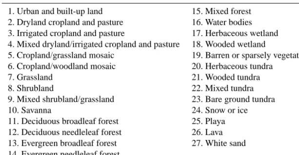
Table 1. The USGS land cover classification.
1. Urban and built-up land 15. Mixed forest 2. Dryland cropland and pasture 16. Water bodies 3. Irrigated cropland and pasture 17. Herbaceous wetland 4. Mixed dryland/irrigated cropland and pasture 18. Wooded wetland
5. Cropland/grassland mosaic 19. Barren or sparsely vegetated 6. Cropland/woodland mosaic 20. Herbaceous tundra
7. Grassland 21. Wooded tundra
8. Shrubland 22. Mixed tundra
9. Mixed shrubland/grassland 23. Bare ground tundra
10. Savanna 24. Snow or ice
11. Deciduous broadleaf forest 25. Playa 12. Deciduous needleleaf forest 26. Lava 13. Evergreen broadleaf forest 27. White sand 14. Evergreen needleleaf forest
near-surface air temperature, near-surface specific humidity, near-surface zonal and meridional wind, and surface pres-sure. The temporal resolution is 3 h and the spatial resolution is 0.25◦.
2.2.2 MODIS albedo
The MODerate-resolution Imaging Spectroradiometer (MODIS) albedo product (MCD43C3), produced by data from both TERRA and AQUA polar-orbiting satellites, is evaluated every 16 days in a Level 3 data set, projected onto a 0.05 latitude–longitude Climate Modelling Grid (CMG) (Schaaf et al., 2002). We use total shortwave broadband for white-sky albedo (bihemispherical reflectance under condi-tions of isotropic illumination) and quality flags that include the percentage of snow and the percentage contribution of fine-resolution data. Cescatti et al. (2012) validated MODIS albedo retrievals against in situ measurements across 53 FLUXNET sites and found a good agreement in mean yearly values between retrievals and measurements with a high correlation (r2=0.82).
2.2.3 USGS land use and land cover
The yearly MODIS land cover and land use data within the International Geosphere-Biosphere Programme (IGBP) global vegetation classification scheme have been slightly modified to fit into the land cover classification of the US Ge-ological Survey (USGS) (Anderson, 1976). In this study, land cover types are grouped into 27 types according to the USGS classification, as shown in Table 1.
3 Results
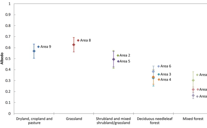
3.1 Physical properties of snow-covered vegetation For figuring out the difference of albedo among various veg-etation types, we select 10 areas within 40–60◦N and 105– 145◦E (Fig. 1) where a single type or two similar types of vegetation occupy more than 70 % in each area (Table 2). In order to minimize the effects of snow cover change, we have averaged the MODIS white-sky albedo over dominating veg-etation type in each area for wintertime (i.e., 273–129 Julian days) in total shortwave broadband during 10 years (2001– 2010) with a 100 % snow cover fraction (SCF) (see Fig. 2). The number of days in each area with a 100 % SCF is suffi-cient for comparison, as shown in Table 3. It is evident that the snow-covered albedo values are distributed over a wide range and relatively low for various forest types. The snow-covered surface albedo is different when the snow is over the ground surface versus over the canopy, mainly due to an un-even structure of the canopy and the forest shading effect. When the growing season is over, leaves disappear for some vegetation (e.g., deciduous trees) and remain unchanged for others (e.g., evergreen trees), while most of stems remain un-changed – reaching the minimum values. Thus, this change at the end of the growing season and the amount of stems depend on vegetation types and make distinctions of albedos over the forest types in winter.
Compared to the MODIS observation, the Noah-MP snow-covered albedos are overestimated over all vegetation types in winter and have little difference between forest and short vegetation (see Table 4). This is mainly due to the use of LAI and SAI, which are not able to quantify leaves and stems representing the forest masking in winter. In the Noah-MP, LAI and SAI are computed as follows:
Table 2. Geographic location, vegetation type, and percentage of dominant vegetation type for selected areas.
Area Longitude Latitude Vegetation type Percentage
1 105.00–107.25◦E 56.50–58.25◦N Mixed forest 71.4 2 116.25–120.00◦E 55.50–57.75◦N Shrubland 80.0
Mixed shrubland/grassland
3 122.50–127.75◦E 57.50–60.00◦N Deciduous needleleaf forest 85.7 4 133.75–136.50◦E 55.75–60.00◦N Deciduous needleleaf forest 90.4 5 138.50–140.75◦E 56.25–60.00◦N Shrubland 82.6
Mixed shrubland/grassland
6 121.25–126.50◦E 53.75–55.75◦N Deciduous needleleaf forest 93.5 7 107.75–111.50◦E 49.00–51.00◦N Mixed forest 81.7 8 113.75–117.75◦E 45.00–49.00◦N Grassland 97.2 9 123.75–127.75◦E 46.75–50.25◦N Dryland cropland and pasture 77.2 10 135.00–137.75◦E 45.00–47.75◦N Mixed forest 93.8
Table 3. Number of days with a 100 % snow cover fraction (SCF) in each area in the period of 2001–2010.
Area 1 2 3 4 5 6 7 8 9 10
No. of days 1483 6159 13 235 12 391 4033 8201 328 9318 7973 248
Figure 1. Geographical locations of the study domain. Each blue
area has a dominant vegetation type as explained in Table 2.
where mleaf (mstem) is the leaf (stem) mass per unit area (in g m−2) and LAPM (SAPM) is the leaf (stem) area per unit mass (in m2g−1). The subscript min implies the min-imum value. The default values of LAImin and SAImin are 0.05 and 0.01 m2m−2, respectively, for all vegetation types. During most of the winter period, both LAI and SAI remain equal to their minimum values (i.e., LAImin and SAImin). Tian et al. (2004) indicated that discrepancies in the winter albedos between the MODIS observation and LSMs were re-lated to the uncertainty in quantifying LAI and SAI in the model. They also mentioned that stems would have different single-scattering albedo than green leaves, and hence it might
be inadequate for the model to treat LAI and SAI the same way in the albedo parameterization.
Figure 3 shows a monthly averaged LAI, calculated from Noah-MP, during the period of 2001–2010 for deciduous broadleaf forest (Fig. 3a), deciduous needleleaf forest (Fig. 3b), and evergreen needleaf forest and mixed forest (Fig. 3c). The red lines represent the minimum, mean, and maximum LAI of the reference values from Asner et al. (2003) for each vegetation type. It is notable that the model-evaluated LAI values are much smaller than the reference values for all veg-etation types in winter. In Fig. 4, the forest SAI has a seasonal cycle in the Noah-MP, but the magnitude is negligibly small. The LAI and SAI in Figs. 3 and 4 have large seasonal vari-ations, even in the case of evergreen needleleaf forest. Such large seasonal variations are directly related to the leaf and stem mass, represented by Eqs. (1) and (2) – see Appendix A for the detailed calculation steps. The leaf and stem mass are reduced in winter because they consider the photosyn-thetic capacity. However, for calculating albedo, the vegeta-tion structure is more important than the photosynthetic ca-pacity, especially in winter.
Figure 2. The MODIS white-sky albedo for total shortwave broadband averaged for winter time in 2001–2010 (dots) and corresponding
standard deviation (bars) when snow cover fraction equals 100 %. Descriptions on the areas are provided in Fig. 1 and Table 2.
Table 4. The values of mean and standard deviation (SD) of snow
albedo from the MODIS observation and the Noah-MP results for the shortwave broadband for different categories of the MODIS land cover. The data are averaged for winter time in 2001–2010 over each vegetation type within 40–60◦N and 105–145◦E with correspond-ing SD when SCF equals 100 % and other snow conditions are the same.
MODIS land cover MODIS Noah-MP
Mean SD Mean SD
Dryland cropland and pasture 0.515 0.088 0.795 0.012
Grassland 0.595 0.080 0.787 0.020
Shrubland 0.432 0.079 0.805 0.029
Mixed shrubland/grassland 0.474 0.085 0.806 0.026 Deciduous broadleaf forest 0.428 0.076 0.748 0.075 Deciduous needleleaf forest 0.346 0.080 0.678 0.134 Evergreen needleleaf forest 0.296 0.097 0.761 0.069 Mixed forest 0.334 0.093 0.721 0.115
includes all leaves, regardless of their ability to express pho-tosynthesis; hence it is higher than the one evaluated by the model, which is related to photosynthesis. Therefore, it is necessary to properly parameterize the vegetation effects on the snow-covered albedo.
3.2 Parameterization of the vegetation effects on the snow surface albedo
We have introduced new parameters in the model – leaf in-dex (LI) and stem inin-dex (SI). LI represents a sum of LAI de-fined in the Noah-MP (i.e., photosynthetic leaves) and LAI of nonphotosynthetic leaves. We have substituted LI with the reference minimum values (see Asner et al., 2003) for four forest types, as shown in Table 5 in Sect. 3.2.2, in order to draw a realistic SI effect. SI represents a sum of SAI defined in the model (i.e., photosynthetic stems) and SAI of non-photosynthetic stems. In defining SI, we assumed that trees were mature and focused on winter when the growing sea-son is over; thus SI has no seasea-sonal cycle. To figure out how albedo responds to stems, we examine the sensitivity of win-ter albedo to SI over forest types in the Noah-MP and then validate albedo with the optimal SI value.
Figure 3. Monthly averaged LAI in the Noah-MP during the period
of 2001–2010 for (a) deciduous broadleaf forest (DecB), (b) de-ciduous needleleaf forest (DecN), (c) evergreen needleleaf forest (EverN), and mixed forest (Mix). The red lines represent the mini-mum, mean, and maximum LAI of the reference values. In (c), the reference values are shown only for EverN.
penetrates through the vegetation without being intercepted by any crowns (Niu and Yang, 2004). The modified two-stream approximation (MTSA), which is the first option of the two-stream radiation transfer scheme, explicitly includes the three-dimensional structure of the vegetation canopy by calculating the total canopy gap probability for direct beam,
Pc. It is equal to the sum of the between-crown gap proba-bility, Pbc, which is a function of crown geometric
proper-Figure 4. Monthly averaged SAI in the Noah-MP during the
pe-riod of 2001–2010 for deciduous broadleaf forest (DecB), decidu-ous needleleaf forest (DecN), evergreen needleleaf forest (EverN), and mixed forest (Mix).
ties and the SZA, and the within-crown gap probability,Pwc, which is parameterized on the basis of a modified version of Beer’s law:
Pbc=e−ρtπ R 2/cos(θ0
), (3)
Pwc=(1−Pbc)e−0.5FaHd/cosθ, (4)
Pc=min(1−fveg, Pbc+Pwc), (5) where ρt is the crown density (stems m−2), R is the hor-izontal crown radius, θ is the solar zenith angle, θ0=
tan−1[(b/R)tanθ], and b is the vertical crown radius. Fa is the foliage area volume density (m−1) and is equal to LSAI/(43π R2bρt), where LSAI is the effective leaf and stem area index, through which the effect of clumping of needles into shoots is included (Chen et al., 1991; Niu and Yang, 2004).Hd is the crown depth.fveg is the green vegetation fraction and ranges from 0 to 1. Therefore, if we apply new LI and SI, LSAI is changed and then the canopy gap proba-bility is changed.
Figure 5 depicts the sensitivity of the snow-covered sur-face albedo and each term in albedo equation in the Noah-MP to SI, averaged over four forest types for different SZA. Total albedo by vegetation and ground,fre, is evaluated as
fre=
(
αdc(1−Pc)+αdPc (for direct beam)
αic(1−Kopen)+αiKopen (for diffuse beam), (6)
Figure 5. Sensitivity of the snow-covered surface albedo and each term in the albedo equation in the Noah-MP to SI averaged over four
forest types: (a) total albedo, (b) canopy gap probability, (c) direct albedo and (d) diffuse albedo for visible broadband, and (e) direct albedo and (f) diffuse albedo for near-infrared broadband.
for visible and direct versus diffuse albedo for near-infrared broadband), is explained in detail in Appendix B.
As expected, total albedo over four forest types generally decreases with increasing SI because snow albedo over the vegetated surface is lower than that over the bare soil surface (Fig. 5a). At a fixed SI, albedo represents different patterns for different SZA – with increasing SZA, albedo decreases at relatively low SI while it increases at relatively high SI. Note that there is sufficient ground surface at relatively low SI that can be shaded by the vegetative canopy as SZA increases (Fig. 5b). Thus, at low SI, albedo is highest when the shadow
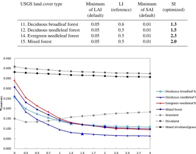
Table 5. Minimum value of LAI, reference values (LI), the default minimum value of SAI, and optimized SI values (in bold) for selected
USGS land cover type (forest). The optimized values are based on the sensitivity test.
USGS land cover type Minimum LI Minimum SI of LAI (reference) of SAI (optimized) (default) (default)
11. Deciduous broadleaf forest 0.05 0.6 0.01 1.3
12. Deciduous needleleaf forest 0.05 0.5 0.01 1.5
14. Evergreen needleleaf forest 0.05 0.5 0.01 2.3
15. Mixed forest 0.05 0.5 0.01 2.0
Figure 6. Sensitivity of the winter-averaged albedo to SI over four forest types and three short vegetation types in the Noah-MP for 2001–
2010. The optimized value for each forest type is indicated with a larger symbol.
3.2.2 Validation of surface albedo with the optimal SI value
For quantifying the forest shading effect through SI in win-ter, we have compared the Noah-MP albedo with observa-tions. We have performed model runs by repeatedly chang-ing SI from 0.0 to 3.0 in order to find the optimal SI for each forest type that is able to reduce the bias of albedo between observation and model output. LAI and SAI were used to cal-culate fluxes of carbon, radiation, turbulent heat, etc., during the growing season. Hence, we have applied LI and SI when the growing season index was off. Albedo has then been aver-aged for 10 years in specific winter days (i.e., 337, 353, and 1, 17, and 33 Julian days) for vegetation types in the East Asia region, in order to compare with the MODIS 16-day obser-vations. We have to priorly evaluate LI for drawing realistic SI effect because LI and SI are considered together for calcu-lating albedo. Here we have assigned the observation values (Asner et al., 2003) to the LI values. Asner et al. (2003) col-lected more than 1000 estimated LAI from literature and then constructed a global LAI data set through a statistical analy-sis. The LAI data set of forest types has been compiled from
plenty of robust samples; thus they are sufficiently reliable to be used as the reference values of LI.
Figure 7. Comparison of RMSE values of albedo with the original minimum value of LAI and SAI (dashed lines) versus new LI and SI (solid
lines) versus observed LAI and prescribed SAI (square symbols) for three radiation options for (a) BATS and (b) CLASS radiation schemes. OPT_RAD1 is MTSA, OPT_RAD2 is two-stream radiation option with no canopy gap, and OPT_RAD3 is the scheme that calculates the gap from vegetation fraction.
errors do not decrease below a certain level is possibly due to other parameters such as snow age, fresh snow albedo, and snow cover fraction that are not validated in the model.
The model performance with the new LI and SI has been evaluated by calculating the root mean square errors (RM-SEs) of albedo against observation (MODIS), as shown in Fig. 7. Here, the RMSEs of albedo, simulated with the ob-served LAI and the prescribed monthly SAI, are also de-picted (square symbols). For the observed LAI, we used the AVHRR GIMSS LAI3g data and took an average for win-ter during 2001–2010 for each vegetation type within the domain of 40–60◦N and 105–145◦E. Since SAI is not ob-served, we have taken the prescribed monthly SAI value in the Noah-MP for each vegetation type. Even with the ob-served vegetation parameter, the RMSEs in simulated albedo are still significant. We have also calculated the RMSEs of
albedo, using the LAI data from Lawrence and Chase (2007) – another good source of LAI but for eight plant functional types rather than five land cover types used in this study. The simulated albedo with these LAI showed larger RMSEs than those with satellite-retrieved LAI (not shown).
There are three radiation options in the Noah-MP for cal-culating energy fluxes (see Fig. 7) – the first is MTSA, employed for parameterization in this study, which calcu-lates canopy gaps from three-dimensional structure and solar zenith angle (OPT_RAD1). The second option is two-stream radiation option with no canopy gap, which means leaves are evenly distributed within the grid cell with a 100 % vegeta-tion fracvegeta-tion (OPT_RAD2). The last is the tile approach that computes energy fluxes in vegetated fraction and bare frac-tion separately and then sums them up weighted by fracfrac-tion (OPT_RAD3). The optimal LI and SI obtained through the MTSA had the similar improving effect on albedo when ap-plied to the other options. The RMSEs with the original min-imum values of LAI and SAI increase until mid-winter (e.g., the 17th Julian day) and decrease after that. During the win-ter, albedo is dominantly influenced by the snow cover and forest masking (Bonan, 2008; Essery et al., 2009; Brovkin et al., 2013). The Noah-MP overestimates snow cover fraction and underestimates vegetation parameters (i.e., LAI and SAI) related to albedo; therefore, albedo is greatly overestimated. This error is significantly reduced by applying new parame-ters that consider all the forest structure effect with realistic values.
4 Conclusions
In winter, albedo has a large variation due to snow cover; however, in forest regions, the snow-covered albedo remains low for two reasons. First, when the snow covers a
for-est canopy, the incident radiation is diffused rather than re-flected due to irregular surfaces. Second, vegetation shields the snow-covered surfaces. In addition, in regions with aver-age December–January–February temperatures greater than
Appendix A: Calculation of the leaf and stem mass The simulated LAI and SAI in the Noah-MP have large sea-sonal variations, even in the case of evergreen forests. This is because LAI and SAI are defined as the photosynthetic active indices. When the growing index is off, both the foliage pho-tosynthesis parameter and the value of the carbon assimilated
(CARBFX; g m−2) become zero. Then, the leaf assimilation
after removing the respiration losses (ADDNPPLF; g m−2) also becomes zero. Thus, in winter, the leaf mass is reduced. The stem mass is calculated in the same way. The equations for calculating leaf and stem mass are shown in the follow-ing:
ADDNPPLF = MAX(0.,LEAFPT*CARBFX - GRLEAF-RSLEAF)
ADDNPPST = MAX(0.,STEMPT*CARBFX - GRSTEM-RSSTEM)
NPPL = MAX(ADDNPPLF,-LFDEL) NPPS = MAX(ADDNPPST,-STDEL) LFMASS = LFMASS +
(NPPL-LFTOVR-DIELF)*DT STMASS = STMASS + (NPPS-STTOVR-DIEST)*DT
where ADDNPPST is the stem assimilation after remov-ing the respiration losses (g m−2),NPPL(NPPS) is the leaf (stem) net primary productivity (g m−2s−1), and LFMASS
(STMASS) is the leaf (stem) mass (g m−2). The LEAFPT
is fraction of carbon allocated to leaves, and STEMPT is fraction of carbon flux to stem. The GRLEAF (GRSTEM) is the growth respiration rate for leaf (stem) (g m−2s−1),
RSLEAF is the leaf maintenance respiration per time step
(g m−2), and RSSTEMis the stem respiration (g m−2). The
LFDEL(STDEL) is the maximum leaf (stem) mass available
to change (g m−2s−1),LFTOVR(STTOVR) is the leaf (stem) turnover per time step (g m−2),DIELF(DIEST) is the death of leaf (stem) mass per time step (g m−2), andDTis a time step (s).
Appendix B: Calculation of total albedo and weights by the radiation components
We here discuss how the radiation components in Fig. 5 are weighted to calculate the total albedo. First, the downward solar radiation (SWDOWN; W m−2) is divided into four parts – direct visible (SOLAD(1)) and diffuse visible (SOLAI(1)) radiation, and direct near-infrared (SOLAD(2)) and diffuse near-infrared (SOLAI(2)) radiation, as shown in the follow-ing equations:
! direct vis
SOLAD(1) = SWDOWN*0.7*0.5 ! direct nir
SOLAD(2) = SWDOWN*0.7*0.5 ! diffuse vis
SOLAI(1) = SWDOWN*0.3*0.5 ! diffuse nir
SOLAI(2) = SWDOWN*0.3*0.5
Second, four albedo components are weighted to calculate the total radiation as follows:
RVIS = ALBD(1)*SOLAD(1) + ALBI(1)*SOLAI(1) RNIR = ALBD(2)*SOLAD(2) + ALBI(2)*SOLAI(2) FSR = RVIS + RNIR
whereALBD(1)andALBD(2)are albedos from direct vis-ible bands and direct near-infrared bands, respectively, and
ALBI(1)and ALBI(2)are albedos from diffuse visible
bands and diffuse near-infrared bands, respectively. RVIS
andRNIRare reflected radiative fluxes from visible bands and near-infrared bands, respectively, andFSR is total re-flected radiative flux. Finally, the total albedo is obtained through the following formula:
ALBEDO = FSR/SWDOWN,
Acknowledgements. This work is supported by the National
Research Foundation of Korea grant (no. 2009-0083527) funded by the Korean government (MSIP). The authors thank Seung-bum Hong at the National Institute of Ecology, Korea, for assistance with the Noah-MP.
Edited by: J. Fyke
References
Anderson, J. R.: A Land Use and Land Cover Classification System for Use With Remote Sensor Data, Vol. 964, US Government Printing Office, Washington, 1976.
Asner, G. P., Scurlock, J. M., and Hicke, J. A.: Global synthesis of leaf area index observations: implications for ecological and remote sensing studies, Global Ecol. Biogeogr., 12, 191–205, 2003.
Bonan, G. B.: Forests and climate change: forcings, feedbacks, and the climate benefits of forests, Science, 320, 1444–1449, 2008. Brovkin, V., Boysen, L., Raddatz, T., Gayler, V., Loew, A., and
Claussen, M.: Evaluation of vegetation cover and land-surface albedo in MPI-ESM CMIP5 simulations, J. Adv. Model. Earth Syst., 5, 48–57, doi:10.1029/2012MS000169, 2013.
Cescatti, A., Marcolla, B., Vannan, S. K. S., Pan, J. Y., Ro-man, M. O., Yang, X., Ciais, P., Cook, R. B., Law, B. E., Matteucci, G., Migliavacca, M., Moors, E., Richardson, A. D., Seufert, G., and Schaaf, C. B.: Intercomparison of MODIS albedo retrievals and in situ measurements across the global FLUXNET network, Remote Sens. Environ., 121, 323–334, 2012.
Chen, J. M., Balck, T. A., and Adams, R. S.: Evaluation of hemi-spherical photography for determining plant area index and ge-ometry of a forest stand, Agr. Forest Meteorol., 56, 129–143, 1991.
Dickinson, R. E., Henderson-Sellers, A., and Kennedy, P. J.: Biosphere–Atmosphere Transfer Scheme (BATS) version 1e as coupled to the NCAR Community Climate Model, NCAR Tech. Note NCAR/TN-387+STR, Natl. Cent. for Atmos. Res., Boul-der, CO, 80 pp., 1993.
Essery, R.: Large-scale simulations of snow albedo mask-ing by forests, Geophys. Res. Lett., 40, 5521–5525, doi:10.1002/grl.51008, 2013.
Essery, R., Rutter, N., Pomeroy, J., Baxter, R., Stahli, M., Gustafs-son, D., Barr, A., Bartlett, P., and Elder, K.: An evaluation of for-est snow process simulations, B. Am. Meteorol. Soc., 90, 1120– 1135, 2009.
Gao, F., Schaaf, C. B., Strahler, A. H., Roesch, A., Lucht, W., and Dickinson, R.: MODIS bidirectional reflectance distribution function and albedo Climate Modeling Grid products and the variability of albedo for major global vegetation types, J. Geo-phys. Res., 110, D01104, doi:10.1029/2004JD005190, 2005. Hardy, J. P., Melloh, R., Robinson, P., and Jordan, R.: Incorporating
effects of forest litter in a snow process model, Hydrol. Process., 14, 3227–3237, 2000.
Henderson-Sellers, A. and Wilson, M. F.: Surface albedo data for climatic modeling, Rev. Geophys., 21, 1743–1778, doi:10.1029/RG021i008p01743, 1983.
Jin, Y., Schaaf, C. B., Gao, F., Li, X., Strahler, A. H., Zeng, X., and Dickinson, R. E.: How does snow impact the albedo of vegetated land surfaces as analyzed with MODIS data?, J. Geophys. Res., 29, 12.1–12.4, doi:10.1029/2001GL014132, 2002.
Lawrence, P. J. and Chase, T. N.: Representing a new MODIS con-sistent land surface in the Community Land Model (CLM 3.0), J. Geophys. Res., 112, G01023, doi:10.1029/2006JG000168, 2007. Lundquist, J. D., Dickerson-Lange, S. E., Lutz, J. A., and Cristea N. C.: Lower forest density enhances snow retention in regions with warmer winters: A global framework developed from plot-scale observations and modeling, Water Resour. Res., 49, 6356–6370, doi:10.1002/wrcr.20504, 2013.
Niu, G.-Y. and Yang, W.-L.: Effects of vegetation canopy processes on snow surface energy and mass balances, J. Geophys. Res., 109, D23111, doi:10.1029/2004JD004884, 2004.
Niu, G.-Y., Yang, Z.-L., Mitchell, K. E., Chen, F., Ek, M. B., Barlage, M., Kumar, A., Manning, K., Niyogi, D., Rosero, E., Tewari, M., and Xia, Y.: The community Noah land surface model with multiparameterization options (Noah-MP): 1. model description and evaluation with local-scale measurements, J. Geophys. Res., 116, D12109, doi:10.1029/2010JD015139, 2011. Qu, X. and Hall, A.: What controls the strength of snow-albedo feedback?, J. Climate, 20, 3971–3981, doi:10.1175/JCLI4186.1, 2007.
Rodell, M., Houser, P. R., Jambor, U., Gottschalck, J., Mitchell, K., Meng, C.-J., Arsenault, K., Cosgrove, B., Radakovich, J., Bosilovich, M., Entin, J. K., Walker, J. P., Lohmann, D., and Toll, D.: The Global Land Data Assimilation System, B. Am. Meteorol. Soc., 85, 381–394, doi:10.1175/BAMS-85-3-381, 2004.
Schaaf, C. B., Gao, F., Strahler, A. H., Lucht, W., Li, X., Tsang, T., Strugnell, N. C., Zhang, X., Jina, Y., Muller, J.-P., Lewis, P., Barnsley, M., Hobson, P., Disney, M., Roberts, G., Dunderdale, M., Doll, C., d’Entremont, R. P., Hu, B., Liang, S., Privette, J. L., and Roy, D.: First operational BRDF, albedo nadir reflectance products from MODIS, Remote Sens. Environ., 83, 135–148, 2002.
Sellers, P. J.: Canopy reflectance, photosynthesis and transpiration, Int. J. Remote Sens., 6, 1335–1372, 1985.
Tian, Y., Dickinson, R. E., Zhou, L., Zeng, X., Dai, Y., My-neni, R. B., Knyazikhin, Y., Zhang, X., Friedl, M., Yu, H., Wu, W., and Shaikh, M.: Comparison of seasonal and spatial variations of leaf area index and fraction of absorbed photo-synthetically active radiation from Moderate Resolution Imaging Spectroradiometer (MODIS) and Common Land Model, J. Geo-phys. Res., 109, D01103, doi:10.1029/2003JD003777, 2004. Verseghy, D. L.: CLASS-A Canadian land surface scheme
for GCMS: I. Soil model, Int. J. Climatol., 11, 111–133, doi:10.1002/joc.3370110202, 1991.
Wang, Z. and Zeng, X.: Evaluation of snow albedo in land models for weather and climate studies, J. Clim. Appl. Meteorol., 49, 363–380, 2010.
Yang, Z.-L., Dickinson, R. E., Robock, A., and Vinnikov, K. Y.: Validation of the snow submodel of the biosphere–atmosphere transfer scheme with Russian snow cover and meteorological ob-servation data, J. Climate, 10, 353–373, 1997.