STUDY ON WAX DEPOSITION RATE OPTIMIZATION ALGORITHM
BASED ON LEVENBERG-MARQUARDT ALGORITHM AND GLOBAL
OPTIMIZATION
Rongge Xiao
a, Yue Zhu
b,*, Wenbo Jin
a, Zheng Dai
a, Shifang Li
a, Fan Zhang
ca
Shaanxi Key Laboratory of Advanced Stimulation Technology for Oil & Gas Reservoirs, College of Petroleum Engineering, Xi’an Shiyou University, Xian, Shaanxi, 710065, China
b
PetroChina Changqing Oilfield Shaanxi, 710018, China
c
China Huanqiu Contracting&Engineering Co.,Ltd.Beijing Huanqiu Corporation, China
A
BSTRACTIn order to accurately obtain the wax deposition rate model, according to the kinetic principle of wax deposition, several factors affecting the wax deposition rate were selected, and by a optimization software of First Optimization(1stOpt), The parameters of two typical wax deposition rate models are solved respectively based on optimization algorithm combined by Levenberg-Marquardt(L-M) algorithm and global optimization and the calculated data were compared. The results show that: compared with the model parameters obtained by least squares method, the model parameters obtained by this optimization algorithm can describe the variation of wax deposition rate more accurately. The maximum error is reduced from 30% to 10%, and the average error is reduced from 10.3% to 2.42%; Alike, the mathematical model obtained by this optimization algorithm is also better than that solved by L-M algorithm alone. The maximum error is reduced from 13.62% to 11%, and the average error is reduced from 6.46% to 4.77%. To a certain extent, this optimization algorithm avoids the premature phenomenon caused by using Levenberg-Marquardt alone. In addition, the use of the optimization algorithm does not require suitable initial values, prior knowledge and programming, easy to use, and has important use value.
Key words: Oil pipeline; Wax deposition rate; mathematical model; optimization algorithm; error analysis
* Corresponding Author. E-mail: [email protected]. 1. INTRODUCTION
The wax component in crude oil will bring a series of problems to the production and transportation of crude oil (Huang Z al., 2011; Azevedo L F A al., 2003; Tian Z al., 2014; Xiao R G al., 2018). In order to find countermeasures, accurate acquisition of wax deposition rate model has become an important part of wax deposition research (Tian Z al., 2014; Zheng S al., 2017; Wang W al., 2014; José P al., 2015). However, the models of wax deposition rate are all nonlinear models, which are usually complex and difficult to obtain model parameters, which greatly restricts the engineering application and development of the models. Scholars have made a detailed study on this issue (Zeng M X al., 2012; Ji Z Y al., 2016). Zhou Shiyan et al first established the wax deposition rate model with the stepwise regression analysis method, but this method can only solve the linear relationship and has low precision (Zhou S D al., 2003; Zhou S D al., 2004). Then, the wax deposition rate model is calculated by artificial neural network method. The calculation result of this method has good accuracy, but the biggest disadvantage of using this method is that the expression of the wax deposition rate model can not be obtained. Wang Junliang et al selected the second-order particle swarm optimization algorithm to obtain the wax deposition rate model (Wang J L al., 2009). The calculation results of this method also have good accuracy, but the method needs to determine the range of regression coefficients, that is, the prior knowledge needs to be calculated before the model calculation. Liu Yongfeng et al established a grey prediction model for the wax
deposition rate of crude oil in pipelines by using the grey system theory, which can avoid the objective problem of unreasonable deviation of the overall prediction results caused by one-sided investigation of individual factors affecting wax deposition (Liu Y F al., 2012; Lou B W al., 2018). However, the wax deposition rate is a constant variable, and the model established by grey system theory is a static model. Therefore, in order to make the model more accurate, it is necessary to establish a dynamic grey prediction model (Liu Y F al., 2012). Kamari and Yan Wenbo et al used the least squares support vector machine to predict the wax deposition rate (Kamari A al., 2013; Kamari A al., 2014; Jin W B al., 2014). This method is similar to the stepwise regression analysis. It is necessary to convert the wax deposition rate model into a linear equation and then complete the sample learning. Finally, the prediction can be made. The use is more complicated. Li Chuanxian et al used L-M method of non-linear multiple regression analysis to study the wax deposition rate model (Li C X al., 2016). This method can obtain good fitting results without depending on the initial value and prior knowledge. However, premature phenomena still inevitably exist when using this method, so that the analytical value obtained is not optimal (Zeng M X al., 2013).
The optimization algorithm combining L-M algorithm and global optimization has been successfully applied in many fields. For example, the calculation of the correction coefficient of the number of dynamic sounding hammer strikes of heavy and super-heavy power in geological exploration of hydropower projects, and the calculation of the dynamic model parameters of diesel hydrodesulfurization. Therefore, it can be proved that this optimization algorithm has certain advantages when
Frontiers in Heat and Mass Transfer
studying nonlinear models. Although the wax deposition rate models are all non-linear models, it has not been seen that this algorithm is applied to the study of wax deposition rate models. In this paper, the optimization algorithm combined L-M algorithm and global optimization is used. Based on 1stOpt mathematical optimization analysis software, the parameters of the model were obtained and the wax deposition rate was predicted. Finally, the comparison with the calculation results of the model in the literature proves the reliability of this optimization algorithm in the establishment of wax deposition rate model. The research results have practical significance for the accurate prediction of wax deposition rate and the establishment of the optimal pigging cycle.
2. INTRODUCTION TO ALGORITHM
2.1 L-M
L-M is not only an effective method to solve nonlinear fitting problems, but also one of the most frequently studied and used methods in the field of solving nonlinear equations. The main principle of this method is to determine whether the objective function achieves the best fitting effect by setting a reasonable objective function and using the iterative program to calculate the sum of squared residuals. If the sum of squares of residuals reaches the minimum value, the iteration process ends and the best fitting function is obtained. The advantage of this method is that it has a faster convergence speed near the minimum point, so it can find the optimal solution quickly (Li H Z al., 2015).
For the data fitting problem of the nonlinear model in practical engineering, the reasonable objective function can be set to calculate the sum of the residuals of the nonlinear function. thus, the prediction of wax deposition rate becomes the nonlinear least squares problem (Li H Z al., 2015). The specific steps are as follows:
1) Definition of objective function.
( )
T( ) ( )
Minimizef x
R
x R x
(1)Where,
R x
( )
y
p( )
x
y
m( )
x
,x
is the position variable;( )
p
y
x
,y
m( )
x
, respectively the predicted value vector and the real value vector of wax deposition rate under the corresponding position variable.2) Partial derivative of the objective function. The objective function takes the first partial derivative of an unknown variable
x
.
( )
2
( )
T( )
f x
R x
R x
(2)Similarly, the objective function finds the second-order partial derivative of the unknown variable
x
.
2
( )
2
( )
T( )
2 ( )
f x
R x
R x
B x
(3)Where,
B x
( )
is the second-order partial derivative of the objective function Hessian matrix, which can be calculated from the following formula:2
( )
m i( )
i( )
i
B x
R x
R x
(4)3) Search direction. In order to minimize the objective function, let the first-order partial derivative of the objective function be 0, scilicet
( )
0
f x
x
, letn
x
be an approximation of the minimum point ofthe objective function, then the approximation
is:
f
f
n 2f x x
n( ,
n)
0
, Let search directionx
x
nbe
D
n, then2
n n n
f D
f
(5)Substitute equation (5) into equation (3), and get
R x( )TR x( )+B x
Dn
R x( )
TR x( ) (6) Equation (6) is the Newton method. SinceB x
( )
is difficult to calculate,B x
( )
is ignored and the above formula becomes:
R x( )TR x( )
Dn
R x( )
TR x( ) (7)Where
x
n1
x
n
a D
n n;a
n is the step size. Equation (7) is the Gauss-Newton Method.Gauss-Newton Method is a typical parameter estimation method, but it is difficult to select the initial value of the algorithm. By introducing the damping factor based on the Gauss-Newton method, Lenvenberg-Marquad proposed the L-M, which not only inherited the global optimization characteristics of Gauss-Newton method, but also broadened the selection range of initial values (Department of Computational Mathematics., 2004; Xie Z et al., 2006).
L-M algorithm as follows:
( )T ( ) n
( )
T ( )n
R x R x u I D R x R x
(8)
Where,
u
n
0
. 2.2 Global OptimizationThe global optimization method studies the characteristics of the global optimum point of the objective function in a certain region and its calculation method (Li H Z al., 2015). Global optimization problems can generally be expressed as
min
( ), . .
Global
f x s t X
S
(9)Where S is a feasible domain, is a non-empty set in
R
n; and( )
f x
is an objective function, which is a real-valued functiondefined on S. If there is one
0
, for allx
x
*
(x
S
) that is satisfiedf x
(
*)
f x
( )
,x
*
S
is a global minimum(Li H Z al., 2015).Although some people began to study the problem now called global optimization in the 1960s, most people's attention at that time focused on linear programming and nonlinear programming localized numerical algorithms. The local optimization algorithm is far more mature than the global optimization algorithm, and has the characteristics of general easy implementation. However, its search performance depends entirely on the neighborhood function and the initial point, and it cannot avoid falling into the local minimum during the search process. Therefore, without the improvement of search strategy, it is impossible to achieve global optimum in most cases. Now the global optimization algorithm is becoming mature and perfect, Grossmann and Floudas have made outstanding contributions in this respect (Wang H T et al., 2009).
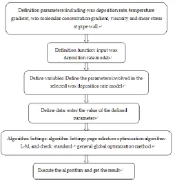
3. IMPLEMENTTATION STEPS OF FITTING PARAMETERS OF OPTIMIZATION ALGORITHM COMBINED WITH L-M ALGORITHM AND GLOBAL OPTIMIZATION
The 1stOpt mathematical optimization analysis software has the L-M algorithm and its computational core is global optimization. Therefore, 1stOpt software was used in this paper for parameter fitting of wax deposition kinetic model, and the steps are shown in figure 1.
4. SELECTION OF REPRESENTATIVE WAX DEPOSITION RATE MODEL AND ANALYSIS OF CALCUTION RESULTS
deposition. Finally, the parameters in the equation are calculated by using laboratory test data, and the wax deposition rate model is obtained (Huang Q Y et al., 2003). There are many models of wax deposition rate at home and abroad, among which the Huang Qiyu model is one of the representative models in China.
Fig. 1 Flow chart of fitting parameters of optimization algorithm combined with L-M and global optimization method
Huang Qiyu (Huang Q Y., 2000) has shown that shear dispersion has little effect on wax deposition through a large number of experimental studies. So the effect of shear dispersion can be ignored in the establishment of the model, but the effect of molecular diffusion and oil flow scouring on wax deposition can be taken into account (Gai Y., 2014). Domestic scholars have so far referred to the Huang Qiyu model, whose model expression is:
1
1
nm w
dC
dT
W
k
dT
dr
(10)The model of Liu Chong (Liu C., 2013) is based on the model of Huang Qiyu, considering the adaptability of the wax model to the static waxing situation and the influence of colloid and asphaltene on the wax formation in the oil, which enlarges the application scope and accuracy of wax deposition model, but more parameters should be fitted accordingly. Its model expression is as follows:
1
(
)(
)
n
z m
w
dC
dT
W
k
S
dT
dr
(11)This paper will select these two representative wax deposition kinetic models for parameter optimization research.
4.2 Analysis of calculation results
Based on the existing experimental data, the model parameters are fitted by the optimization algorithm of 1stOpt software: L-M algorithm and global optimization. And the wax deposition rate is calculated and compared with the literature calculation value and experimental value. 4.2.1 Example 1
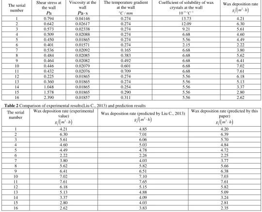
In Liu C., 2013, Liu Chong's model is adopted, and the algorithm used is the least square method. Experimental data in Liu C., 2013 are shown in table 1. The comparison of the wax deposition rate calculated by the optimization algorithm combining the L-M algorithm and global optimization with the experimental value and the literature value is shown in table 2. The error comparison between the fitting model in
this paper and the model in Liu C., 2013 is shown in figure 2, and the average error is shown in table 3.
Using the experimental data in Table 1, the model parameters of this paper are fitted as follows: z=0.429, k=223.719, m=-0.590, n=0.407.
Fig 2 Error comparison between the fitting model in this paper and that in Liu C., 2013
Table 3 Comparison of the average error between the fitting model in this paper and that in Liu C., 2013
Wax deposition kinetic model average error(%) Fitting model in this paper 2.42
Fitting Model in Liu C., 2013 10.3
The error in figure 2 is represented by the absolute value of the error. The average error in table 3 is the average of the absolute value of the error in figure 2. From Figure 2, we can see that the fitting model error in this paper is much smaller than that in Liu C., 2013. Combining with Fig. 2 and Table 3, we can see that the maximum error of the fitting model is only 10%, the average error is only 2.42%, which is less than 30% of the maximum error in literature 26 and 10.3% of the average error. The above data shows that the wax deposition rate model established by the optimization algorithm combined with the L-M algorithm and global optimization is far superior to the wax deposition rate model established by the least squares method.
4.2.2 Example 2
In Li C X et al., 2016, Huang Qiyu model is adopted, and the algorithm used is L-M method. The experimental data in Li C X et al., 2016 are shown in Table 4. The comparison of the wax deposition rate calculated by the optimization algorithm combining the L-M algorithm and global optimization with the experimental value and the literature value is shown in table 5. The error comparison between the fitting model in this paper and the model in Li C X et al., 2016 is shown in figure 3, and the average error is shown in table 6.
Using the experimental data in Table 4, the model parameters of this paper are fitted as follows: k=859.523, m=-0.182, n=-0.253. Table 6 Comparison of the average error between the fitting model in this paper and that in Li C X et al., 2016
Wax deposition kinetic model average error(%) Fitting model in this paper 4.77
Fitting Model in Li C X et al., 2016 6.67
superior to the wax deposition rate model established by the L-M alone. This is because the general global optimization method avoids the premature phenomenon caused by the single use of the L-M to a certain extent.
Fig 3 Error comparison between the fitting model in this paper and that in Li C X et al., 2016
5. CONCLUSION
(1) The optimization algorithm combining the L-M algorithm and global optimization based on 1stOpt software is used to establish the wax deposition rate model without giving an appropriate initial value, prior knowledge or programming. The method is simple and efficient.
(2)Two representative wax deposition models were studied by the optimization algorithm combining the L-M algorithm and global optimization based on 1stOpt software.and the accuracy of the results obtained is better than that calculated in the original literature. On the one hand, the accuracy of this method is verified, which can provide more accurate and reliable wax deposition rate mathematical model for pipeline operation and management of waxy crude oil. On the other hand, it also proves that the algorithm is universal for non-linear multiple regression problems, and is also suitable for solving other regression problems.
Table 1 Experimental data in Liu C., 2013
The serial number
Shear stress at the wall
a
P
Viscosity at the wall
a s
P
The temperature gradient at the wall
/
o
C mm
Coefficient of solubility of wax crystals at the wall
4 1
10 o
C
Wax deposition rate
2
g m h
1 0.794 0.04146 0.274 13.73 4.21
2 0.642 0.02617 0.274 12.09 6.30
3 0.573 0.02338 0.274 9.21 5.61
4 0.509 0.02088 0.274 6.68 4.60
5 0.450 0.01865 0.274 5.56 4.49
6 0.401 0.01571 0.274 2.15 2.22
7 0.536 0.02092 0.165 6.68 3.80
8 0.484 0.02085 0.383 6.68 5.62
9 0.464 0.02082 0.492 6.68 6.41
10 0.446 0.02079 0.601 6.68 7.02
11 0.432 0.02076 0.709 6.68 7.61
12 0.225 0.01865 0.274 5.56 6.18
13 0.360 0.01865 0.274 5.56 5.13
14 1.048 0.01865 0.254 5.56 3.37
15 1.578 0.01865 0.290 5.56 2.80
16 2.390 0.01857 0.311 5.56 2.62
Table 2 Comparison of experimental results(Liu C., 2013) and prediction results
The serial number
Wax deposition rate (experimental value)
2
g m hWax deposition rate (predicted by Liu C., 2013)
2
g m h
Wax deposition rate (predicted by this paper)
2
g m h1 4.21 4.85 4.20
2 6.30 7.01 6.39
3 5.61 6.06 5.70
4 4.60 5.03 4.84
5 4.49 4.78 4.72
6 2.22 2.26 2.25
7 3.80 4.03 3.77
8 5.62 5.82 5.66
9 6.41 6.51 6.38
10 7.02 7.10 7.03
11 7.61 7.65 7.61
12 6.18 5.15 5.82
13 5.13 4.88 5.09
14 3.37 4.09 3.24
15 2.80 4.03 2.81
Table 4 Experimental data in Li C X et al., 2016
The serial number
Shear stress at the wall
a
P
Viscosity at the wall
a s
P
The temperature gradient at the wall
/
o
C mm
Coefficient of solubility of wax crystals at the wall
4 1
10 o
C
Wax deposition rate
2
g m h
1 0.188861 0.009454 0.234 0.298 3.176
2 0.258919 0.011400 0.233 2.751 26.343
3 0.336705 0.030899 0.233 15.276 47.137
4 0.422100 0.038720 0.231 26.480 67.288
5 0.299496 0.011909 0.133 2.751 13.987
6 0.208870 0.011210 0.323 2.751 32.127
7 0.161441 0.010862 0.422 2.751 45.600
8 0.104553 0.011527 0.234 2.751 30.663
9 0.165964 0.011527 0.234 2.751 27.853
10 0.397579 0.011372 0.240 2.751 23.705
Table 5 Comparison of experimental results(Li C X et al., 2016) and prediction results
The serial number
Wax deposition rate (experimental value)
2
g m hWax deposition rate (predicted by Li C X et al., 2016)
2
g m h
Wax deposition rate (predicted by this paper)
2
g m h1 3.176 3.529 3.518
2 26.343 29.080 25.343
3 47.137 47.241 48.491
4 67.288 64.980 65.274
5 13.987 15.892 15.537
6 32.127 34.744 34.212
7 45.600 44.439 45.192
8 30.663 29.474 29.667
9 27.853 27.298 27.269
10 23.705 26.686 24.019
ACKNOWLEDGEMENT
This work was supported by the Special Funding Project of Shaanxi Province Industrial Science and Technology Project (NO. 2015GY094) and Xi'an Petroleum University Youth Science and Technology Innovation Fund (NO. 2015BS011), so grateful here.
NOMENCLATURE
W
—Wax deposition per unit time per unit area of pipe wall,
2
g m h
w
—Shear stress in crude oil at the wall,Pa
—Viscosity of crude oil at the wall,Pa s
dCdT
—The "solubility coefficient" of wax crystals in oil, that is, the
temperature drop 1o
C, the wax crystals account for the mass fraction of crude oil, o 1
C dT
dr
—Radial temperature gradient of crude oil at the wall, o
/
C mm
S
—The sum of mass fractions of asphaltene and resin in crude oil;
—Equivalent shear stress,Pa
; k,z,m,n—Coefficient to be regressed.REFERENCES
Azevedo L F A, Teixeira A M., 2003, “A Critical Review of the Modeling of Wax Deposition Mechanisms,” Liquid Fuels Technology, 2003, 21(3-4): 16.
https://doi.org/10.1081/LFT-120018528
Department of Computational Mathematics, Tongji University., 2004,
“Modern numerical mathematics and computation,” Tongji University Press, 56-209.
Gai Y., 2014, “Study on Wax Deposition Model of Waxy Crude Oil Pipeline,” Master's thesis, Southwest Petroleum University.
Huang Q Y., 2000, “Study on the Dynamic Model of Wax Deposition in Waxy Crude Oil Pipeline,” Ph.D. Thesis, Beijing: China University of Petroleum.
Huang Q Y, Zhang J J, Yan D F., 2003, “A New Wax Deposition Model,” Oil & Gas Storage and Transportation, 22(11): 22-25.
Huang Z, Lee H S, Senra M, Fogler H S., 2011, “A fundamental model of wax deposition in subsea oil pipelines,” Aiche Journal, 57(11): 2955-2964.
https://doi.org/10.1002/aic.12517
Jin W B, Jing J Q, Tian Z, Sun N N, Wu H F., 2014, “Prediction of wax deposition rate based on least squares support vector machine,” CHEMICAL INDUSTRY AND ENGINEERING PROGRESS, 33(10): 2565-2569.
http:// doi:10.3969/j.issn.1000-6613.2014.10.008
José P, Cabanillas, Leiroz A T, Azevedo L F A., 2015, “Wax Deposition in the Presence of Suspended Crystal,” Energy & Fuels, 30(1).
https://doi.org/10.1021/acs.energyfuels.5b02344
Ji Z Y, Li C X, Yang F, Cai Jin Yang, Cheng L, Shi Y N., 2016, “An experimental design approach for investigating and modeling wax deposition based on a new cylindrical Couette apparatus,” Liquid Fuels Technology, 34(6): 8.
Kamari A, Khaksar-Manshad A, Gharagheizi F, Mohammadi A,H, Ashoori s., 2013, “Robust Model for the Determination of Wax Deposition in Oil Systems,” Industrial & Engineering Chemistry Research, 52(44).
http://dx.doi.org/doi:10.1021/ie402462q.
Kamari A, Mohammadi A H, Bahadori A, Zendehboudi S., 2014, “A Reliable Model for Estimating the Wax Deposition Rate During Crude Oil Production and Processing,” Liquid Fuels Technology, 32(23):2837-2844.
https://doi.org/10.1080/10916466.2014.919007
Liu Y F, Wu M, Jiang Y M, Lv L., 2012, “Grey system theorybased wax deposit rate prediction model for oil pipeline,” Oil & Gas Storage and Transportation, 31(1): 17-19.
http:// doi:CNKI:13-1093/TE.20110914.1340.001
Liu C., 2013, “Research on the characteristic of Rotary Facility of the Wax Deposition and the Law of Wax Deposition of Crude Oil,” Master's thesis, Beijing: China University of petroleum.
Li H Z, Guo F, Pan Y Z, Xie S Y, Xiao Y H., 2015, “Study on extension and polynomial fitting of correction factors of heavy dynamic penetration and extra heavy dynamic penetration,” Yangtze River, 1: 30-35.
doi:10.16232/j.cnki.1001-4179.2015.01.008
Li C X, Ji Z Y, Yang F, Cai J Y, Chen H, Li S, Shi Y L., 2016, “Study on wax deposition of Changqing crude oil based on a newly developed Couette device,” Journal of China University of Petroleum, 40(6):135-142.
doi:10.3969/j.issn.1673-5005.2016.06.017
Lou B W, Wang P Y, Xu S, Chen Y, Liu H S, Duan J M., 2018, “Research progress of wax deposition in single-phase oil pipeline,” Oil & Gas Storage and Transportation, 37(08): 857-864.
http:// doi:10.6047/j.issn.1000-8241.2018.08.003
Tian Z, Jin W B, Wang L, Jin Z., 2014, “The study of temperature profile inside wax deposition layer of waxy crude oil in pipeline,” Frontiers in Heat and Mass Transfer (FHMT), 5(1).
http:// doi:10.5098/hmt.5.5
Tian Z, Jin W B, Zhou L, AAn Y P, Wu H F., 2014, “Prediction of wax deposition rate in pipeline by BP neural network,” Journal of Xi'an Shiyou University( Natural Science Edition), 29(1): 66-70.
doi:10.3969/j.issn.1673-064x.2014.01.013
Wang J L, Wang Y H., 2009, “Optimization Study on Wax Deposition Rate Model,” Oil & Gas Storage and Transportation, 28(6): 36-37.
Wang H T, Wang H, Chai X F., 2009, “Study on kinetics model of diesel hydrodesulfurization,” CHEMICAL INDUSTRY AND ENGINEERING PROGRESS, 28(5).
doi:10.16085/j.issn.1000-6613.2009.05.018
Wang W, Huang Q., 2014, “Prediction for wax deposition in oil pipelines validated by field pigging,” Journal of the Energy Institute, 87(3): 196-207.
https://doi.org/10.1016/j.joei.2014.03.013
Xie Z, Li J P, Tang Z Y., 2006, “Nonlinear Optimization. The 2 edition,” Changsha: National Defense and science and technology University.
Xiao R G, Jin W B, Tian Z, She Y T, Wang L., 2018, “The Study on Calculation Method of Temperature Distribution of Tested Tube for Wax Deposition Experimental Loop,” Frontiers in Heat and Mass Transfer (FHMT), 10.
https://doi.org/10.5098/hmt.1012
Zhou S D, Jiang G Y, Wu M., 2003, “MStepwise Regression Model of Wax Sediment Veloeity,” JOURNAL OF FUSHUN PETROLEUM INSTITUTE, 23(4): 27-30.
Zhou S D, W M, W J., 2014, “Wax deposition rate model for crude oil pipeline based on neural network,” Journal of Xi’an Shiyou University(Natural Science Edition), 19 (1): 38-40.
Zeng M X, Song Y G., 2012, “Study on the Influencing Factors of the Levenberg-Marquardt Algorithm for X-ray Diffraction Quantitative Phase Analysis,” ROCK AND MINERAL ANALYSIS, 31(5): 798-806. doi::10.15898/j.cnki.11-2131/td.2012.05.004
Zeng M X, Song Y G., 2013, “Application of the Levenberg-Marquardt Algorithm to X-Ray Diffraction Quantitative Phase Analysis,” Earth Science-Journal of China University of Geosciences, 38(2): 431-440. doi:10.3799/dqkx.2013.043
Zheng S, Saidoum M, Palermo T, Mateen K, Fogler H S., 2017, “Wax Deposition Modeling with Considerations of Non-Newtonian Characteristics: Application on Field-Scale Pipeline,” Energy & Fuels, acs. Energyfuels, 7b00504.