SYSTEMATIC STRATEGY FOR MODELING AND OPTIMIZATION OF
THERMAL SYSTEMS WITH DESIGN UNCERTAINTIES
Po Ting Lin, Hae Chang Gea, Yogesh Jaluria
*Mechanical and Aerospace Engineering, Rutgers University, Piscataway, New Jersey, 08854, USA
A
BSTRACTThermal systems play significant roles in the engineering practice and our lives. To improve those thermal systems, it is necessary to model and optimize the design and the operating conditions. More importantly, the design uncertainties should be considered because the failures of the thermal systems may be very dangerous and produce large loss. This review paper focuses on a systematic strategy of modeling and optimizing of the thermal systems with the considerations of the design uncertainties. To demonstrate the proposed strategy, one of the complicated thermal systems, Chemical Vapor Deposition (CVD), is simulated, parametrically modeled, and optimized. The operating conditions, inlet velocities and susceptor temperatures, are the most significant factors in the CVD and are chosen as the design variables. Several responses - including the percentage of the working area, the mean of the deposition rate, the root mean square of the deposition, and the surface kurtosis - are chosen based on the physical needs and statistical foundations, and are utilized to represent the productivity and the quality of the thin-film deposition. One of the Response Surface Method (RSM), the Radial Basis Function (RBF), is employed to formulate the objective and constraint functions for the optimization. However, it is not until the design uncertainties are considered that the thermal system designs have high risk of the violations of the performance constraints. The Reliability-Based Design Optimization (RBDO) algorithms are used to solve the optimization problems with the design uncertainties. The most famous RBDO methods are the Reliability Index Approach (RIA) and the Performance Measure Approach (PMA). In RBDO, probabilistic constraints are established with respect to either normally or non-normally distributed random variables. The optimal solutions are found subjected to the allowable level of the failure probabilities. The Monte Carlo Simulation (MCS) results can be used to evaluate the failure probabilities. As a result, the proposed systematic strategy of parametrically modeling and optimizing with design uncertainties can be applied to either experiments or simulations of other thermal systems to quantitatively represent the performances, improve their productivity, maintain the quality control, and reduce the probability of the system failure.
Keywords: Chemical Vapor Deposition (CVD), Response Surface Method (RSM), Radial Basis Function (RBF), Reliability-Based Design Optimization (RBDO), Reliability Index Approach (RIA), Performance Measure Approach (PMA)
* Corresponding author. Email: [email protected]
1.
INTRODUCTION
Thermal systems not only are essential technologies in engineering practice but also play significant roles in our lives. With the continuously growing needs of the thermal systems in many different applications, such as power systems, air conditioning, energy conversion, chemical processing, material processing, aerospace, and automobiles, the design and the optimization of the thermal systems have become very important research works in the engineering field.
The thermal systems are often very complicated because of the complex physics and mechanics involved in the systems, including fluidic mechanics, heat transfer, mass transfer, and chemical reactions. It is nearly impossible to realize the closed-form relationships between the system performances and all the involved variables. Therefore, it is important to firstly understand the basic characteristics of the thermal systems and subsequently determine the principal design variables which dominantly control the system performances.
A systematic strategy is then desired to model and optimize the thermal systems. This proposed strategy must be able to resolve the following questions:
• How to model the system performances in terms of the design variables so that the system performances can be accurately described by the proposed models?
• How to formulate the optimization problems in terms of the defined models for improving the system performances? In the aspect of the modeling, the mathematical models that are able to quantitatively and literally represent the physical behaviors of the system performances are necessary. With the desired models, the optimization problems can then be formulated to achieve the goals of the thermal system designs.
Unfortunately, the existence of the design uncertainties is unavoidable. A traditional deterministic optimization algorithm often leads the optimal solution to the boundaries of the active constraints. Without the considerations of the design uncertainties, the optimal solution from the deterministic optimization formulation is unreliable and has high probabilities of violating the active constraints. Therefore, additional attentions should be drawn to the optimization problems with the design uncertainties and the following questions should be answered:
• How to formulate a non-deterministic optimization problem when the design variables are uncertain?
Frontiers in Heat and Mass Transfer
• How to solve this non-deterministic optimization problem and how to solve it efficiently?
2.
THERMAL SYSTEMS
As described earlier, the thermal systems are very important in various applications and our lives. To design and optimize the thermal systems, the most fundamental step is to recognize their existence and classify them into different groups in terms of their functionalities. A common classification of the thermal system is given as follows (Jaluria, 1998):
• Manufacturing and materials processing systems.
• Energy systems.
• Cooling systems for electronic equipment.
• Environmental and safety systems.
• Aerospace systems.
• Transportation systems.
• Air conditioning, refrigeration, and heating systems.
• Fluid flow systems and equipment.
• Heat transfer equipment.
• Other thermal systems.
After understanding the physics and the mechanics behind the thermal systems, the control variables are chosen to determine the system performances. Therefore, the decision of the design variables is the key factor of the modeling and the optimization of the thermal systems.
Manufacturing and Materials Processing Systems:
Heattransfer plays an important role in the manufacturing and materials processing systems, where the materials often change their mechanical properties due to temperature changes. The controls of the temperature changes determine the productivity and the quality of the processes. Examples include crystal growing, metal casting, metal forming, plastic injection molding, etc. (Jaluria, 1998) One of those processes, the Chemical Vapor Disposition (CVD) process, will be considered in the later sessions. A systematic strategy to design and optimize the CVD process with design uncertainties will be proposed and it can be applied to the design and the optimization of other thermal systems.
Energy Systems
have become one of the most important thermalsystems in recent years in which the thermodynamics of the energy conversions are the issues of most concern. Energy systems are often very complicated because they contain several subsystems, such as energy collector, steam generator, turbines, condenser, etc. (Van Wylen and Sonntag, 1986) Numerous design variables should be considered to improve the thermal efficiency of the energy system.
Cooling Systems
are essentially important for electronic equipment where the operating temperatures are constrained within certain allowable temperatures (Steinberg, 1980). Other constraints for the cooling systems include the spatial working space, the allowable noise, etc. The objective of the cooling system design is often minimizing the ratio of used power to reduced temperature, while the design variables are often the geometries of the heat sink which differ the surface area of the heat transfer (Yang and Peng, 2008; 2009).Environmental and Safety Systems:
Safety is an important factorfor systems with extreme environmental conditions, such as high temperature and toxicity. Environmental and safety systems include the applications for heat rejection to air or water, control of the temperature and the pollution of thermal systems, etc. The heat rejection from a power plant is a good example while the heat is dumped to the river as a cooling pond. The operation of the power plant will be under high risks if the safety systems fail. Therefore, the safety system should be taken into careful consideration in the design of the systems with extreme environmental conditions.
Aerospace Systems:
Thermal systems are the most importantcomponents in aerospace systems, such as rockets, turbines, etc. For an instance of the rocket system, the alcohol/water mixture is pumped into the combustion chamber to heat the fuel and cool the chamber. The balance between the high thrust for launching and the efficient cooling is the focus in the design of the rocket systems.
Transportation Systems
cannot operate without the existence of the thermal systems, including diffusion, compression, combustion, turbine, and nozzle systems. In a turbine engine, the thrust energy comes from the combustion of the air/fuel mixture. Thermodynamics is significant for the design of the transportation systems (Van Wylen and Sonntag, 1986), while they are often optimized in terms of maximizing the ratio of the generated power to utilized fuel.Air conditioning, Refrigeration, and Heating Systems
areindispensable to our daily lives. Detailed information about such kind of the thermal systems can be found in the references of (Stoecker and Jones, 1982; Kreider and Rabl, 1994). Take the air conditioning system as an example, the physical phase, the temperature, and the pressure of the fluid change via the mechanisms of the condenser, the evaporator, and the compressor. The optimization for such thermal systems often focuses on decreasing the power consumption and improving the efficiency of the temperature control.
Fluid Flow Systems and Equipment
include hydrauliccomponents, such as pumps, turbines, compressors, fans, etc. Fluid mechanics is of the major concern in the fluid flow systems and is closely related to the thermal systems with energy transmission, cooling, and mass transfer (Fox and McDonald, 1992). One of the examples is a wastewater treatment system in which the waste water is transferred through several different fluid mechanisms, clarified, and delivered to the drainage system.
Heat Transfer Systems
contain heat exchangers (Kays and London,1984), furnaces, heaters, condensers, etc. The most straightforward example is the heat exchangers where the heat is transferred to the water to increase its temperature for human usage. The design of the heat exchanging mechanisms considers the transmission of the energy and the control of the heat loss.
There is never a best way to classify all kinds of the thermal system but the most practical ones have been covered and discussed. In the later session, one of the materials processing systems, the CVD process, is taken into consideration. The design and the optimization of the CVD process will be studied and a systematic strategy will be proposed to implement the modeling and the optimization of the CVD process with design uncertainties. The proposed methodology is expected to have the capability of designing and optimizing of the other thermal systems.
3.
Chemical Vapor Deposition Processes
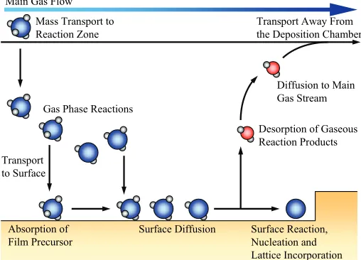
Main Gas Flow
Gas Phase Reactions
Transport to Surface
Absorption of Film Precursor
Surface Diffusion Surface Reaction, Nucleation and Lattice Incorporation
Desorption of Gaseous Reaction Products
Diffusion to Main Gas Stream Transport Away From the Deposition Chamber Mass Transport to
Reaction Zone
Fig. 1 Schematic sequence of steps in CVD process (Mahajan, 1996).
3.1.
Different Applications of the CVD Processes
The CVD-based products have become more and more important in our daily lives because of the high quality of the deposited thin layers with various kinds of materials. The CVD process is well utilized to produce highly uniform thin films deposited on different kinds of substrates (typically 0.01 to 10 μm) (Mahajan, 1996). It is used in a wide range of applications where thin coatings of high purity are required.
The CVD processes can be utilized to produce high-quality microstructures in semiconductors, special materials with dielectric properties as insulators, and metallic conductors with different resistivities. Furthermore, the CVD processes generate high-strength products such as protective coatings, anticorrosive coatings, and ceramic materials. Besides the productions of thin layers, it is possible to generate powers and fibers of different materials by the CVD processes. Other applications such as optical materials and synthetic diamonds have high qualities and purities of different materials. The common materials in different applications of the CVD processes are listed in Table 1. Most of the research interests in the later discussions is directed at the CVD of silicon because of its relevance to the semiconductor industry (Gardeniers et al., 1989; Breiland and Coltrin, 1990).
3.2.
Different Types of the CVD Processes
CVD processes can be classified in terms of their operating conditions or different kinds of instruments. With different operating pressures of the CVD reactors, the CVD processes include three different types:
• Atmospheric Pressure CVD (APCVD).
• Low-Pressure CVD (LPCVD).
• Ultra-High Vacuum CVD (UHVCVD).
The APCVD operates at the pressure of 0.1 to 1 atm while the LPCVD works at a lower pressure of 10−3atm (Mahajan, 1996). Other
modern CVD processes reach high or ultra-high vacuum (below
6
10− Pa) and have high-quality thin-film depositions.
Table 1 Common materials in different applications of the CVD processes (Sherman, 1987; Gardeniers et al., 1989; Breiland and Coltrin, 1990; Fotiadis et al., 1990; Creighton and Parmeter, 1993; Gladfelter, 1993; Rebenne and Bhat, 1994; Cheng et al., 1995; Hintermann, 1996; Mahajan, 1996).
Different CVD
Applications Common Materials
Semiconductors silicon (Si), gallium arsenide (GaAs) Dielectrics silicon dioxide (SiO2), silicon nitride (Si3N4) Metallic conductors
tungsten silicide (WSi2), molybdenum silicide (MoSi2), tungsten (W), aluminum
(Al), molybdenum (Mo), polysilicon (Si) Protective coatings molybdenum (Mo), gold (Au), platinum (Pt) titanium nitride (TiN), Tungsten (W),
Ceramics
aluminum oxide (Al2O3), titanium carbide (TiC), silicon carbide (SiC), boron carbide
(B4C), titanium biboride (TiB2) Anticorrosive
coatings for turbine blades
boron nitride (BN), molybdenum disilicide (MoSi2), silicon carbide (SiC), boron carbide
(B4C) Powers for sintering
and hot pressing silicon nitride (Si3N4), silicon carbide (SiC) Fibers for
composite materials
boron (B), boron carbide (B4C), silicon carbide (SiC)
High-purity monolithic materials for infrared optics
zinc selenide (ZnSe), zinc sulfide (ZnS), cadmium sulfide (CdS), cadmium telluride
(CdTe) Synthetic diamonds carbon (C) Table 2 Different types of the CVD processes.
Different
Types Descriptions
Plasma-Enhanced
CVD (PECVD)
A CVD instrument with plasma enhancement where higher density of reactant species are produced to the
substrate due to the high-energy electron impact. Higher activity of the gaseous species allows deposition at comparatively low temperature (450 to
650 K). (Sherman, 1987; Mahajan, 1996)
Metal-Organic CVD (MOCVD)
Also known as Organo-Metallic Vapor Phase Epitaxy (OMVPE). An epitaxial growth of materials from
the surface chemical reaction of organic or metal-organic compounds and an important process for the manufacturing of solar cells and LEDs. (Stringfellow,
2001; Kurtz et al., 2007) Laser CVD
(LCVD)
A laser-assisted instrument that locally heat the substrate to activate the CVD reaction with precise
control. (Allen, 1981)
Photo CVD (PCVD)
A photo-assisted deposition technique where UV or visible photon energies are used for gas decomposition. The deposition at very low temperature (300 to 450 K) is allowed but having a low deposition rate and poor uniformity. (Eden, 1991;
Mahajan, 1996) Chemical
Vapor Infiltration
(CVI)
A variant CVD device that deposits within a porous body and is widely used for the fabrication of ceramic materials. (Naslain and Langlais, 1986) Hot Wire
CVD (HWCVD)
A special instrument for producing high-temperature gas decomposition but room-temperature deposition
on the substrate. (Lau et al., 2001) Atomic
Layer CVD (ALCVD)
A technology to produce ultrathin layers of crystalline materials (typically 1 to 50 nm). (Nilsen,
Another method to classify the CVD processes considers the operating wall temperature of the CVD chamber. They are:
• Cold-Wall CVD.
• Hot-Wall CVD.
Most of the CVD processes operate with the hot-wall reactors and the gaseous temperature is distributed uniformly inside the reactor. The advantage of the hot-wall setting is higher deposition rate and better uniformity of the deposition. On the other hand, the cold-wall setting allows higher throughput and easier cleaning but has lower speed of the deposition and poor uniformity of the thin film.
In the consideration of different instruments, a wide variety of CVD processes have been developed, listed in Table 2. Plasma-assisted CVD processes operate at low pressure and allow the cold-wall setting because the plasma bombards the gas mixture and decompose into active species for deposition at low temperature. Photo CVD is another instrument that works at low temperature and uses the activation energy from ultraviolet or visible photons to achieve the gaseous decomposition. Laser CVD is a device that provides higher activation energy and, furthermore, very accurate control of the local deposition. Other CVD instruments like Metal-Organic CVD (MOCVD) and Chemical Vapor Infiltration (CVI) have specific applications. The epitaxial growths of III/V materials from MOCVD have become very important in the manufacturing of solar cells and light-emitting diodes (LEDs), and the semiconductors with organo-metallic compounds. CVI is the specific instrument for the growth of ceramic materials in a porous body.
3.3.
Different Configurations of the CVD Reactors
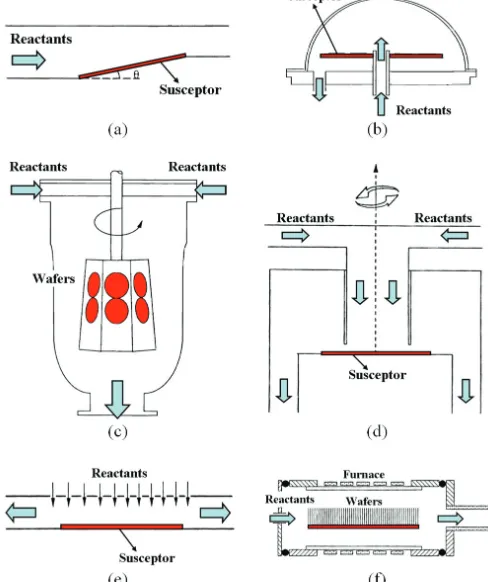
For different operating conditions and applications, several different configurations of the CVD reactors have been developed. The Fig. 2 illustrates some common CVD reactors. Typically, the reactors in Fig. 2 (a), (b), and (c) are utilized for cold-wall settings and the ones in Fig. 2 (d), (e), and (f) have higher wall temperatures of the CVD chambers. The barrel reactor has been greatly used for the huge-amount production of the silicon epitaxial wafers. The vertical reactor with rotating susceptor is often utilized for single-wafer depositions; on the other hand, the one in Fig. 2 (e) has higher area of uniform deposition and is used for the depositions of multiple wafers. The tubular reactor is usually used to deposit films with polysilicon and dielectric materials. In the later discussion, the modeling and the optimization of the CVD processes focus on the configuration of the vertical impinging reactor with the stationary susceptor in Fig. 2 (e).
In the design and optimization of the CVD processes, different design variables should be taken into consideration for different configurations. For example, the horizontal reactor in Fig. 2 (a) has a tilt angle of the susceptor for uniform deposition with horizontal gaseous flow of the reactant species. The rotation speeds of the reactors in Fig. 2 (c) and (d) differ the quality of the deposition. The directions of the reactant flow above the susceptor certainly provide different characteristics of the fluidic mechanics and heat transfer. Among all configurations of the CVD reactors, there are some common variables that dominate the performance of the thin-film deposition, including the concentration of the gaseous reactant in the inlet flow, the velocity of the inlet flow, the temperature of the susceptor, the temperature of the chamber wall, the operating pressure in the CVD chamber, etc. The review about the design of the CVD processes will be given in the next subsession.
4.
Design of the CVD Process
Different designs of the CVD processes have a wide variety of the film thickness, generally ranges from a few nanometers to tens of microns. As described previously, the film formation process is highly dependent on the flow and the heat transfer between the gas and the heated substrate. Therefore, in order to produce thin films with higher deposition rates and quality, the operation conditions must be studied.
There are two major aspects to be considered in the design of the CVD processes:
• Experiments or simulations of the CVD processes.
• Modeling of the responses.
Reviews about those aspects are given in the following.
Fig. 2 Different configurations of the CVD reactors: (a) horizontal reactor, (b) pancake reactor, (c) barrel reactor, (d) vertical impinging reactor with rotating susceptor, (e) vertical impinging reactor, and (f) tubular reactor. (Mahajan, 1996)
Table 3 Typical design variables and responses in the CVD designs. (Dimitrios et al., 1987; Fotiadis et al., 1990; Jensen et al., 1991; Mahajan, 1996; Chiu and Jaluria, 2000; Chiu, Richards et al., 2000)
Design Variables Responses
Hardware settings
Susceptor size
Shape of CVD chamber Angle of susceptor vs.
the flow direction Orientation of
susceptor vs. gravity Buoyancy driven /
force driven flow Diffusivity of susceptor
material
Deposition thickness Deposition rate Deposition uniformity Nusselt number Temperature
distribution of the susceptor
Purity of the deposition Composition of the
deposition Adhesion to the
substrate
Surface morphology Grain structure in the
deposition Distance of flow
separation Operating
conditions
Velocity of inlet flow Susceptor temperature Operating pressure Rotation speed of the
susceptor
4.1.
Design Variables and Responses of the CVD
Processes
Once the reactant species, the type of the CVD process, and the CVD configuration have been determined for the desired thin-film production on the susceptor, several operating parameters should be chosen to perform the experiments or the simulations of the CVD process. Among those parameters, some of them dominate the control of the deposition performance and are selected to be the design variables. The typical design variables are categorized into two different types, including hardware settings and operating conditions, and listed in Table 3. The hardware settings vary the boundary conditions and the mechanical properties of the fluid mechanics and the heat transfer in the CVD processes. On the other hand, the operating conditions are the quantitative variables to control the behavior of the reactant fluid and the performance of the deposition. Besides the hardware and operating design variables, the rest of the parameters remain constant because of either their minor impacts to the deposition or the simplicity of the CVD design. In this research work, the inlet velocity and the susceptor temperature are chosen as the design variables because their quantities can be easily controlled by the designers.
The merit of the deposition performance requires several quantitative responses to judge, where those responses typically have physical meanings and provide numerical measures. Table 3 points out several common responses from either the experiments or the simulations of the CVD processes. Among those typical responses, some of them still lack of numerical measures to decisively quantify its degree of intensity. For example, the deposition uniformity itself is a subjective scale of the quality of the CVD production. George (George, 2007) utilized a weighted sum of the local slopes of the deposition to quantify its uniformity. Lin et al. (Lin, Jaluria et al., 2009) used some standard statistical measures, including the root mean square and the kurtosis, as the responses of the uniformity factors. More details about the chosen design variables and the significant responses will be discussed in the later session.
4.2.
Experiments or Simulations of the CVD Processes
The mechanics of the CVD process, in which the flow, the heat transfer, and the chemical reaction are involved, is very complicated. The flow in the CVD process has firstly been visualized by seeding micro-scale titanium dioxide (TiO2) particles in the reactant gas and illuminating by laser (Wahl, 1977; Giling, 1982; Wang et al., 1986). However, the holography observation using the laser provided poor resolution of the lowly concentrated reactants. On the other hand, numerical simulations provide relatively better understanding of the fluid mechanics and have become very important to study the complex flow in CVD process.
Numerous researchers have been devoted to investigate the flow and heat transfer in CVD reactors. Some of them focused on the simulations of the horizontal CVD reactors (Moffat and Jensen, 1986; Fotiadis et al., 1990; Karki et al., 1993; Chiu, Richards et al., 2000; Chiu et al., 2001), while many other important studies have been conducted to the vertical configurations (Sugawara, 1972; Dimitrios et al., 1987). Among all the numerical analysis in CVD reactors, three major governing equations are considered – continuity, momentum, and energy conservations (Patankar, 1980). Generally, parabolic governing equations (Moffat and Jensen, 1986; Quazzani and Rosenberger, 1990) are utilized to predict the flow pattern in CVD reactors. However, extreme conditions, such as low Reynolds numbers and high density gradients, lead to reverse flow (Visser et al., 1989) which required elliptic governing equations for better predictions (Quazzani and Rosenberger, 1990; Karki et al., 1993).
Simulations of the CVD processes are very complicated because of huge amount of controlling variables (Raja et al., 2000), complicated analysis of the fluidic dynamics and the kinetics of the chemical reactions, and all the variable properties (Jensen et al., 1991) to be
considered. Numerical models with constant properties (Eversteyn et al., 1970; Gebhart et al., 1988; Spall, 1996) and Boussinesq approximations (Gray and Giorgini, 1976; Gebhart et al., 1988) have been utilized to simplify the complex simulations. Wang et al.. (Wang et al., 2003) and Chiu et al. (Chiu, Jaluria et al., 2000) demonstrated that the constant-property models are acceptable for most practice but variable-property models give more accurate predictions for extreme operating conditions. The Buoyancy effect has been neglected when the ratio of Grashof number and square of Reynolds number is less than two (Quazzani et al., 1988; Chiu and Jaluria, 1997). The geometry of the reactor is also a factor in the fluid dynamics of the CVD process but it is negligible in a large aspect ratio (Chiu, Jaluria et al., 2000). The temperature distribution of the susceptor is approximated to be isothermal for some CVD configurations (Chiu and Jaluria, 1997).
Thorough comparisons between the experiment and simulation results are provided by Dimitrios et al. (Dimitrios et al., 1987) and Chiu et al. (Chiu et al., 2001). Comprehensive reviews on CVD reactor studies are given by Mahajan (Mahajan, 1996) and Jensen et al. (Jensen et al., 1991). Kee et al. (Kee et al., 1995; Raja et al., 2000) demonstrated that model simulations have much greater flexibility and versatility as compared to experimental counterparts. Experimental studies have also been carried out on the flow in channels for CVD applications (Jensen et al., 1991; Chiu, Richards et al., 2000; Chiu et al., 2001; Chiu et al., 2002).
4.3.
Optimization of the CVD Processes and Existence of
the Design Uncertainties
Simulation and optimization of CVD systems have been studied by many researchers (Mouche et al., 1995; Southwell et al., 1996; Chiu, 1999; Raja et al., 2000; Chiu et al., 2002; Ly and Tran, 2002; George, 2007; Lin, Jaluria et al., 2009). However, design uncertainties can found everywhere in the CVD process. Even if an optimal design is obtained from the optimization models, the irresistible uncertainties will cause unstable responses of the CVD process. For example, the compositions of the deposition species have errors of 15 % (Mitchell et al., 1997). Several researchers have estimated the randomness of the operating parameters in the CVD process. The rate constant of the chemical reaction may have a wide variance; for example, 10 to 13
14
10 cm3/mol-s (Goodwin, 1993). In this research work, the existence of the design uncertainties is considered at the design variables, the inlet velocity and the susceptor temperature of the CVD process.
The main contribution of this research includes
• The development of the performance responses in the CVD process.
• The parametric modeling of those responses in terms of the chosen design variables.
• The optimization formulations of the operating operations for the CVD process.
• The realization of the convergence problem in a traditional RBDO algorithm, the TRIA.
• The development of the MRIA to solve optimization problems with normally distributed design uncertainties.
• The development of the MRIA for the non-normally distributed random variables.
• The application of the MRIA on the RBDO problems of the CVD process.
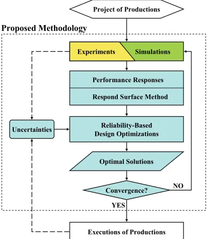
The Fig. 3 schemes the systematic strategy to parametrically model the responses from the experiments or the simulations of the thermal systems and optimize the operating conditions with design uncertainties using the proposed RBDO algorithm.
responses with respect to the design variables. Optimization problems are formulated in terms of the RSM models and are utilized to provide the operating conditions for higher productivity and quality of the productions. Due to the existence of the design uncertainties, the traditional deterministic optimization formulation is no longer reliable to generate safe designs because it may lead to a design with high risk of system failure. The development of the Reliability-Based Design Optimization (RBDO) algorithm evaluates the probabilities of the system failures and provides a more conservative design which reaches to the optimality as the failure probabilities are subject to some acceptable level. Finally, the productions of the thermal systems are executed based on the optimal design variables. If any design uncertainties are found in the experiments, the simulations, or the mass productions, the information of the uncertainties are fed back to the formulation of the RBDO problems and new optimal conditions can be generated by the proposed strategy.
Simulations
Performance Responses
Respond Surface Method
Reliability-Based Design Optimizations
Convergence? NO
YES
Project of Productions
Optimal Solutions Uncertainties
Experiments
Executions of Productions
Proposed Methodology
Fig. 3 Flowchart of the proposed systematic strategy.
5.
SIMULATION AND RESPONSES OF THE CVD
PROCESS
This session is directed at the simulation of the CVD process and the responses of to represent the productivity and the uniformity of the deposition. The effect of different operating conditions on the deposition rate and the film quality are identified from the numerical simulations performed using a commercial software, FLUENT. The simulation of the thin-film growth of silicon from the reactant of silane in a vertical impinging CVD reactor is discussed. The design operating conditions focus on the velocity of the inlet flow and the temperature of the susceptor. Four different responses are defined in terms of the design variables and measured from the simulated deposition profiles to represent the performances of the silicon deposition.
5.1.
Simulation of the CVD Process
A schematic of the vertical impinging CVD reactor is shown in Fig. 4. The reaction gases are introduced at the top in a vertical impinging reactor, while the flow is assumed to be two-dimensional steady laminar flow (Chiu and Jaluria, 1999). The flow with a dilute precursor concentration of silane in hydrogen as the carrier gas deposits
silicon onto the susceptor. Silane decomposes to silicon and hydrogen on the susceptor following a one-step reaction mechanism. The conservations of continuity, momentum, and energy are considered, shown by Eqs. (1), (2), and (3) respectively. Furthermore, the species conservation, shown by Eq. (4), is studied where there are three species, silane, silicon, and hydrogen, in the CVD chamber.
0
v
∇ ⋅ = (1)
( )
(
)
v⋅∇ ρv = ∇ ⋅ ∇ + − ∇μ v F p (2)
(
ρC vTP)
(
kT T)
Q∇ ⋅ = ∇ ⋅ ∇ + (3)
(
ρvm)
(
ρD m)
R∇ ⋅ = ∇ ⋅ ∇ + (4)
where v is the velocity of the flow, T is the temperature, m is the mass fraction of species, ρ is the density, μ is the dynamic viscosity, CP is the specific heat, kT is the thermal diffusivity, D
is the mass diffusivity, F is the body force, ∇p is the pressure difference, Q is the heat source, and R is the production rate of species.
Reaction gases entering reactor (Silane + Hydrogen) Reaction gases entering reactor
(Silane + Hydrogen)
SiH4(g)Si(s)+ 2H2(g)
H2(g) H2(g)
H2(g) H2(g)
Isothermally heated susceptor
2cm 6cm 2cm
2cm
Fig. 4 Vertical impinging CVD reactor (George, 2007; Lin, 2010). Simulations are carried out employing the commercial software FLUENT using the laminar finite-rate model, which computes the chemical source terms using Arrhenius expressions and ignoring the effects of turbulent fluctuations. (Lin, 2010) In the FLUENT model, both gas phase and wall surface reactions are considered, while the reaction rate is given by an Arrhenius expression, shown as follows
(
)
exp a g
ATα E R T
κ = − (5)
where κ is the rate constant, A=0.334 is the pre-exponential factor, T is the temperature, 1 105
a
E = × is the activation energy, 0.5
α= is the temperature exponent, and Rg is universal gas constant. The material properties are given by the FLUENT database. The usage of FLUENT can accommodate different geometries and boundary conditions, providing more flexibility and saving more research time.
so they are considered as the design variables in this case study. The velocity and temperature bounds are taken from 0.1 to 1 m/s and 400 to 1500 K respectively. Only half of the fluid domain is considered in the simulation due to the geometrical symmetry while four-node quad meshes are utilized – totally 320 139× nodes. Node density is chosen such that the solution is independent to the number of elements. For one typical simulation, it takes around 10 minutes to converge in an Intel® Pentium® M processor 2.0 GHz with 2.0 GHz of RAM.
Outflow Inflow; T = 300 K;
Fraction of SiH4 = 0.1;
Vin(m/s)
Non-slip wall; Tsus(K) Non-slip wall; T = 300K Non-slip wall; T = 300K
Fig. 5 Boundary conditions of the vertical CVD simulation.
Velocity (m/s)
Vin
Velocity (m/s)
Vin
(a)
Tsus
Temperature (K)
Tsus
Temperature (K)
(b)
Deposition Rate of Si (kg/m2s)
Position of Susceptor (m)
(c)
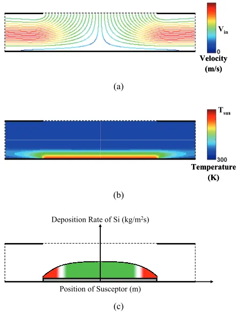
Fig. 6 Typical results of the vertical CVD simulation: (a)
streamlines of the flow, (b) temperature distribution, and (c) scheme of silicon deposition profile (Lin, 2010).
The Fig. 6 (a) shows a typical numerical result of the streamlines in the CVD reactor where the inlet has uniformly distributed velocity,
V, and the stagnation point at the center of the susceptor has zero velocity. The subfigure (b) illustrates the corresponding temperature distribution in the CVD chamber where the susceptor is isothermally heated at the temperature of T and the walls remain room temperature following the boundary conditions. The subfigure (c) shows a scheme of the deposition profile of silicon while the red area has poor uniformity of the deposition rate. The red area is highlighted
when its local slope of the deposition profile is too oblique; on the other hand, only the green area has local slopes very close to zero and the corresponding uniformity is acceptable uniformity.
5.2.
Validation
To validate the correctness of the numerical simulations with the developed settings in FLUENT, the deposition rate of the silicon in a horizontal CVD reactor is compared with experimental and numerical results from other researchers (Eversteyn et al., 1970; Mahajan and Wei, 1991; Chiu and Jaluria, 2000; Yoo and Jaluria, 2002; George, 2007). The Fig. 7 illustrates the configuration of the horizontal CVD reactor and its dimensions. The reactant, the silane, is mixed in the hydrogen carrier flow, with the inlet velocity of 0.175 m/s. The partial pressure of the silane is 124.1 Pa under the atmospheric pressure, providing the information of the mass fraction of the silane. The operating temperature is 300 K and the susceptor is isothermally heated at 1323 K. The material properties and the kinetics of the chemical reactions are given from (George, 2007) otherwise from the FLUENT database. The rest of the settings and the utilized solvers remain the same as the previous discussion.
Reaction gases entering reactor (Silane + Hydrogen)
SiH4(g)Si(s)+ 2H2(g)
Isothermally heated susceptor
5cm 30cm 15cm
2cm
Fig. 7 Horizontal CVD reactor (George, 2007).
The results from the simulation of a horizontal CVD reactor using FLUENT are compared with the experimental results obtained by (Eversteyn et al., 1970) and the numerical results from (Mahajan and Wei, 1991; Chiu and Jaluria, 2000; Yoo and Jaluria, 2002), shown in Fig. 8. A detailed comparison between experimental and numerical results has been made and fairly good agreements has been found (Chiu, 1999). The numerical results using the settings described in the previous discussion is almost identical to George‘s simulation results (George, 2007) with the mass diffusivity in the FLUENT database, which is given by a polynomial equation of the temperature as follows:
8 10 2 14 3
7.234 10 4.569 10 8.016 10
D= × −T+ × − T − × − T (6)
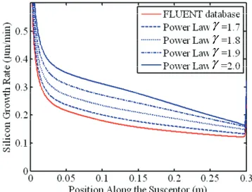
George (George, 2007) has also shown the numerical results are very close to the experimental results in (Eversteyn et al., 1970) if higher mass diffusivity is utilized. Eversteyn et al. (Eversteyn et al., 1970) utilized a power law to describe the mass diffusivity which is given by
(
)
0 300
D D T= γ (7)
where D0 is the pre-exponential factor, γ is the temperature exponent, and the temperature, T , is normalized by the operating temperature, 300 K. Considering the pre-exponential constant in (Yoo and Jaluria, 2002), 5
0 6.24 10
shown in Fig. 10. In this research work, the mass diffusivity is chosen from the FLUENT database.
Simulation (Yoo & Jaluria)
Diffusion-Controlled Simulation (Yoo & Jaluria) Experiment (Eversteyn et al.)
Simulation (Mahajan & Wei) Simulation (Chiu & Jaluria)
Simulation with Increased Mass Diffusivity (George) Simulation with FLUENT Database (George) Present
Simulation (Yoo & Jaluria)
Diffusion-Controlled Simulation (Yoo & Jaluria) Experiment (Eversteyn et al.)
Simulation (Mahajan & Wei) Simulation (Chiu & Jaluria)
Simulation with Increased Mass Diffusivity (George) Simulation with FLUENT Database (George) Present
Fig. 8 Deposition rate of silicon in the horizontal CVD reactor compared with others (Eversteyn et al., 1970; Mahajan and Wei, 1991; Chiu and Jaluria, 2000; Yoo and Jaluria, 2002; George, 2007).
γ γ γ γ
Fig. 9 Mass diffusivity of silane with different temperature exponent compared with FLUENT database.
γ γ γ γ
Fig. 10 Growth rate of silicon in the horizontal CVD reactor with different mass diffusivity.
5.3.
Function Formulations of the Responses in CVD
Process
Some quantitative measures are needed to justify the performance of the deposition profile to achieve higher deposition rate and better film quality on the susceptor during the CVD process. Four responses have been defined in (Lin et al., 2008), including the Percentage of the Working Area (PWA) and three mathematical functions – Mean of Deposition Rate (MDR), Root Mean Square (RMS) and Surface Kurtosis (KUR). The PWA is used because the quality of deposition close to the edge of the susceptor and the working area excludes all un-usable areas. In the working area, the other three response functions represent the productivity and the uniformity of the silicon deposition.
Percentage of Working Area (PWA)
is defined as the ratio of theEffective Working Area (EWA) and the total area in the deposition profile and it is given by
EWA
PWA 100%
Total Area
= × (8)
where the EWA is determined based on the local uniformity check and the continuity of the working area. A local area is considered as workable only when the local slope, S , is very close to zero or it is smaller than an uniformity threshold, SU. In the study of the vertical CVD, the quantity of SU is chosen as a small value, 0.00055 . Normally, regions with higher slopes occur around the edges of the susceptor due to the dramatic temperature drop. However, there are some cases that the uniform areas are located far from the edge and result in discontinuous working areas. Those isolated uniform area cannot be utilized to produce micro-structures. Hence, the EWA is given as the largest set of the working area at the middle of the deposition profile excluding the rest of the isolated working areas. The rest of the responses should be measured within the EWA instead of the entire area of the susceptor because only the deposition performance in the working area is of concern and the non-working area will be dumped.
Mean of Deposition Rate (MDR)
is measured inside the EWA asthe key criteria to represent the performance of CVD process. It is given as
1
1
MDR Q q
q
D
Q =
=
(9)where Q is the number of uniformly distributed sampling nodes within the EWA, and Dq is the deposition rate at the sampling node. The higher MDR represents better CVD productivity. A deposition profile with a larger PWA along with higher MDR is very desirable; however, these two objectives sometimes conflict with each other. In the later session, two different kinds of the optimization formulations will be studied – one maximizes the PWA and the other one maximizes the MDR.
Root Mean Square (RMS) and Surface Kurtosis (KUR):
ThePWA only provides a local measure for uniformity, therefore it is essential to determine the global uniformity mathematically and represent the global physical behaviors of the deposition profile within the EWA. Two statistical measures, the Root Mean Square (RMS) and the Surface Kurtosis (KUR), are utilized to quantify the global uniformity.
(
)
2 11
RMS MDR
Q
q q
D
Q =
=
− (10)which is the standard derivation of the deposition rate of all sampling nodes within the EWA. A deposition profile with large RMS represents un-even uniformity of the thin-film formation even all regions are considered as workable from the PWA point of view. Therefore, the RMS is an important global indicator for the film quality, which is complementary to the local indicator, PWA.
The KUR is the forth statistical moment of the deposition profile and it mathematically implies the existences of the sharper peaks in the deposition profile which cannot be recognized by the RMS. It is measured by
(
)
(
)
4 4
1
1
KUR MDR
RMS Q
q q
D
Q =
=
− (11)where the terms of MDR and the RMS are defined in the Eqs. (9) and (10) respectively. The deposition profile with a higher KUR has greater peakedness or higher variance due to infrequent extreme deviations. A silicon deposition with allowable KUR is desired. Also, the skewness is not considered because the configuration of the vertical CVD reactor is symmetric about the centerline of the inlet flow and the skewness is always zero. For other geometrical configurations, the skewness is also an important factor to study the global uniformity and symmetry.
The percentage of the EWA in the susceptor has been defined to quantify the production yield of the CVD process. The MDR is measured within the EWA to represent the productivity, while the RMS and the KUR are utilized as the indicators of the uniformity inside the EWA. Several samples of the CVD simulations under different operating conditions have been utilized to show the importance of four responses in the quantifications of the productivity and the uniformity of the CVD process. Both RMS and KUR are global measures for the quality of deposition uniformity whereas the PWA and MDR are direct local measures. These four functions are greatly influenced by the inlet velocity and the susceptor temperature. However, the true forms of these functions are not available. Therefore, we will establish response surface models of these functions with respect to the design variables.
5.4.
Parametric Modeling Using Response Surface
Method (RSM)
The best way to represent the behavior of the responses in the CVD processes and model them in terms of numerical functions with respect to the design variables is to use the technique of curve fitting, also known as metamodeling or Response Surface Method (RSM). RSM provides a parametric equation in terms of the design variables and some coefficients to be determined by substituting the experiment / simulation data into the parametric model. Instead of using the common RSM tool, Polynomial Response Surface (PRS), the Radial Basis Function (RBF) is used to model the deposition rate and the uniformity of the deposition profile. These obtained parametric models of the four responses will be validated before being utilized to formulate the optimization problems of CVD process.
Response Surface Method
can be divided into two different types(Jaluria, 1998):
• Exact fitting.
• Best fitting.
The exact fitting is the technique that generates a smooth curve that passes through all the data points. It typically is a function with M
parameters to be determined by the known information from M data
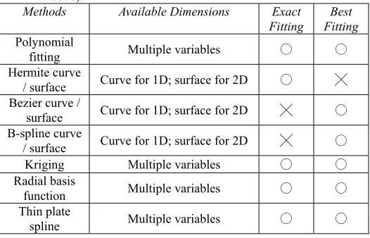
points. Therefore, it is very accurate and useful for small amount of data. On the other hand, the best fitting does not necessarily pass through any of the data points but provides a best prediction of the behavior of the responses. It is very useful when the amount of data points is very large (i.e. There are only K parameters to be determined for M sampling points while K<M.) or the obtained responses are not accurate enough. Several methods have been developed to achieve either exact or best fitting with single variable, two variables, or multiple variables. Table 4 lists different kinds the RSM methods and their characteristics.
Table 4 Different RSM methods (Jaluria, 1998; Van Beers and Kleijnen, 2003; Van Beers and Kleijnen, 2004; Mortenson, 2006).
Methods Available Dimensions Exact
Fitting
Best Fitting
Polynomial
fitting Multiple variables ○ ○
Hermite curve
/ surface Curve for 1D; surface for 2D ○ ╳ Bezier curve /
surface Curve for 1D; surface for 2D ╳ ○ B-spline curve
/ surface Curve for 1D; surface for 2D ╳ ○
Kriging Multiple variables ○ ○
Radial basis
function Multiple variables ○ ○
Thin plate
spline Multiple variables ○ ○
Polynomial Response Surface (PRS)
is the most common andsimple technique to interpolate or extrapolate the obtained responses with M sampling points. For small-scale models, a regression formulation is given as follows:
( )
( )
F x ≅ ⋅w B x (12)
where w is a vector of the K regression coefficients to be determined and B x
( )
is a linear combination of the modeling monomials, shown in Table 5.Table 5 Typical coefficients for PRS.
Different PRS K B x
( )
Linear regression 2
[
1 1]
T
x
Planar regression 3
[
1 x1 x2]
TCoupling 2-D fitting 4
[
1 x1 x2 x x1 2]
TIndependent 2-D quadratic
fitting 5 1 1 2 12 22
T
x x x x
Coupling 2-D quadratic
fitting 6
2 2
1 2 1 2 1 2
1 x x x x x x T
For exact fitting, K=M and the coefficients, w , can be obtained by the following equation:
( ) ( )
1 S S S
−
= ⋅
w A x F x (13)
where FS
( )
xS is a K 1× vector of the responses in terms of the
K sampling points and A x
( )
S is a K Kis
( )
sT S
B x . For best fitting, K<M and FS
( )
xS is a M×1 vector and A x( )
S is a M K× matrix. Instead of using Eq. (13), the coefficients of w need to be obtained by Least Square Approximation (Myers et al., 2009) shown as follows:( ) ( )
1( ) ( )
T S S − T S S S
= ⋅ ⋅ ⋅
w A x A x A x F x (14)
Geometric Modeling Curves and Surfaces:
There are severalfamous geometric modeling methods that can be utilized for the purpose of RSM (Mortenson, 2006). Those include Hermite, Bezier, and B-Spline curves for single-variable RSM and Hermite, Bezier, and B-Spline surfaces for two-variable RSM. A Hermite cubic curve contain multiple continuously connected cubic curves which are parameterized by polynomial functions in terms of four sampling points. The parametric equation is a single-variable polynomial fitting function in Eq. (12) with
( )
2 31 1 1
1 x x x T
=
B x . The advantage
of using a known parametric function like Hermite curve is that the coefficients, w, are given already and no further calculation is needed for the determination of w. However, it is generally used for exact fitting. Bezier and B-spline curves are utilized for best fitting of the responses with different set of coefficients, w. More details are included in (Mortenson, 2006).
Kriging
is a general method to predict the responses from theexperiment or simulation data with minimum error variance estimation (Lebensztajn et al., 2004). It is constructed by an inner product of a vector of coefficients, w, and a covariance vector,
(
, S)
x
C x x , shown
as follows:
( )
(
, S)
x
F x ≅ ⋅w C x x (15)
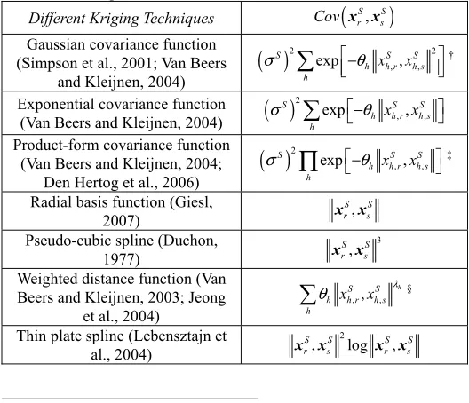
Table 6 Common covariance functions for different Kriging techniques.
Different Kriging Techniques
(
S, S)
r s
Cov x x
Gaussian covariance function (Simpson et al., 2001; Van Beers
and Kleijnen, 2004)
( )
2 2
, ,
exp ,
S S S
h h r h s h
x x
σ
−θ †Exponential covariance function
(Van Beers and Kleijnen, 2004)
( )
2
, ,
exp ,
S S S
h h r h s h
x x
σ
−θ Product-form covariance function (Van Beers and Kleijnen, 2004;
Den Hertog et al., 2006)
( )
2
, ,
exp ,
S S S
h h r h s h
x x
σ
∏
−θ ‡Radial basis function (Giesl,
2007) ,
S S r s
x x
Pseudo-cubic spline (Duchon, 1977) 3 , S S r s x x
Weighted distance function (Van Beers and Kleijnen, 2003; Jeong
et al., 2004)
,, ,
h
S S h h r h s h
x x λ
θ
§Thin plate spline (Lebensztajn et al., 2004)
2
, log ,
S S S S
r s r s
x x x x
† σS stands for the known standard deviation of the responses and h
θ is the unknown correlation parameter to be determined by maximizing the likelihood estimates.
‡ h denotes the index for the important sampling points and there exists more than one important sampling points.
§ λh controls the smoothness of the distance function.
where the covariance vector contains M×1 components of the covariance functions and is given by
(
)
,(
)
(
)
1 1
, S M , S M , S
x x s s s s s
s s
C Cov
= =
=
=
C x x x x e x x e (16)
and es is the sth normal basis. The coefficients of w can be obtained by
( ) ( )
1 S S S
− ⋅
w = C x F x (17)
where
( )
S M1 M1(
S, S)
r s r s r s
Cov = =
=
C x x x e e (18)
is a M M× symmetric matrix with zero diagonal terms and non zero off diagonal terms of covariance functions,
(
S, S)
r s
Cov x x . Many different covariance functions have been utilized for the predictions of the response surfaces and they are listed in The RBF has no approximation error at all sampling points and is expected to provide better approximations of the responses with non-linear behaviors than the simple PRS.. Besides, other available covariance functions are constructed in a class of polynomial functions in terms of the basis function, S, S
r s
x x , shown in (Wendland, 1995). This kind of Kriging technique is utilized for exact fitting. On the other hand, a linear combination of the polynomial fitting function in Eq. (12) and the Kriging function in Eq. (15) makes best fitting possible for Kriging (Simpson et al., 2001). The polynomial term provides the global shape of the response surface, while the Kriging term provides local predictions of the responses.
5.5.
Parametric Modeling of the CVD Responses
Radial Basis Function (RBF)
(Giesl, 2007) is a special kind ofKriging, where the covariance function is the Euclidean distance between two corresponding vectors, namely,
(
S, S)
S, Sr s r s
Cov x x = x x (19)
It is preferred because the approximation of PRS may not be very accurate if the response is highly nonlinear. The RBF approximates the response, F, as a weighted summation of covariance functions:
(
)
1 , M S s s sF w Cov
=
≅
x x (20)where ws is the weighting factor to be determined. Two CVD operation parameters are studied, inlet velocity, V and susceptor temperature, T . The four functions described previously are approximated using the RBF in the design domain which contains M
sampling points, S S S T s =Vs Ts
x for s=1,2, ,M . Therefore, the Eq. (19) is given as
(
, S)
sS 2 sS 2 sm m
V V T T
Cov
V T
− −
= +
x x (21)
m
V =1.0 m/s and Tm=1500 K. The RBF has no approximation error at all sampling points and is expected to provide better approximations of the responses with non-linear behaviors than the simple PRS.
Model Validation:
The RSM needs to be validated before theformulation of the optimization problems. Lin et al. (Lin, Jaluria et al., 2009) studied the RBFs with three different kinds of sampling sets – uniformly distributed 9-point, 13-point, and 25-point designs. In this case study, uniformly distributed sampling is considered but another famous sampling method is the Latin Hypercube Sampling (Stein, 1987). A 437-point response was considered as a benchmark of the true responses. The detailed information of the 437 sampling points can be found in (Lin, 2010). The difference between the studying sample set and the 437-point response is quantified by an error function give as
(
)
437 2
1
1
437 p p
p
err F G
=
=
− (22)where Fp and Gp denote the nodal values of the approximate function and the simulation respectively. The results showed the 25-point design has low errors (less than 4 %) while a 25-25-point polynomial response surface has less accuracy due to the nonlinearity of the responses. For simplicity, the following sessions will use the 25-point RBF.
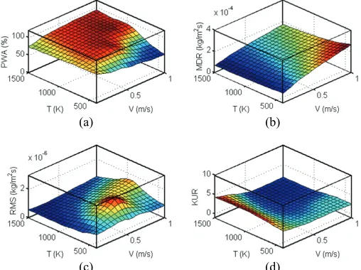
The Fig. 11 demonstrates the 25-point RBFs of the PWA, MDR, RMS, and KUR of the silicon deposition profiles. Due to the occurrence of the isolated working areas at high inlet velocity and low susceptor temperature, a sudden drop of PWA is found around that region. This sudden decrease of the PWA causes non-smooth behaviors during the transition. Unlike the models of PWA, the MDR behavior is very smooth because the MDR is an averaged value in the EWA and any non-linear behavior is blended into the entire function.
(a) (b)
(c) (d)
Fig. 11 25-Point RBFs of (a) PWA, (b) MDR, (c) RMS, and (d) KUR. The proposed RBF can be utilized to parametrically model the responses in any other thermal systems. It is especially useful when the responses are highly nonlinear; otherwise, the polynomial response surface is less complicated and good enough for less nonlinear functions. In the next session, those response surface modeled are to be utilized to formulate optimization problems for enhancing the productivity and the quality of the silicon deposition. Besides obtaining a best set of the operating parameters of the CVD processes, the system reliability at the optimal setting is also an important study.
In practice, the optimal setting is only useful only when the corresponding system reliability is acceptable.
6.
OPTIMIZATION OF THE CVD PROCESS
The response surface models are used to formulate the optimization problems of the CVD process while better operating conditions are expected to be found to improve the performance of the CVD process in this session. The objective and constraint functions are formulated by the RBF models of the CVD responses. For higher productivities, one of the objective functions is to maximize the PWA while another one is to maximize the MDR. On the consideration of the uniformity of the deposition, the RMS and the KUR are subject to certain quantitative levels. Both constraints of the deposition uniformity are very significant to the locations of the optimal operating conditions. Furthermore, the system reliability with respect to the optimal solution is of another significant concern. Without the consideration of the randomness of the system, there exists high risk of system failure when operating the system with the optimal parameters. To overcome this problem, a systematic method is desired to provide more conservative designs than the traditional ones.
6.1.
Problem Formulations
In a general CVD process, the PWA and the MDR should be maximized in order to obtain the highest productivity, and two global uniformity factors, the RMS and the KUR are required to satisfy some desirable guidelines. Therefore, two optimization formulations (Lin et al., 2008) are proposed. The first one is to maximize the PWA with uniformity constraints on the RMS and the KUR while the deposition rate is subjected to a minimum level. The second one is to maximize the MDR with the same uniformity constraints while the PWA must be larger than an acceptable level. The detailed information about the optimal solutions is given later. Other possible formulations are shown in (Lin, 2010).
Example 1a - Maximizing the PWA Subject to Constraint of
Deposition Rate:
The first formulation is to maximize the workingarea on the susceptor subject to the constraints of the global uniformity factors described previously and an additional constraint on the deposition rate. It is expressed as follows:
,
U
U
L
PWA
. . RMS RMS
KUR KUR
MDR MDR
V T
L U
L U
Max
s t
V V V
T T T
≤ ≤ ≤ ≤ ≤ ≤ ≤
(23)
where the limit states of the constraints are taken as
6 U
RMS =1.35 10× − , U
KUR =2.62, and 4 2
L
MDR =1.5 10 kg/m s× − . The chosen bounds are VL=0.2 m/s, VU =0.9 m/s, TL=400 K, and
1400 U
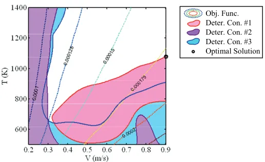
T = K because the interior of the responses surface model has better approximation than its edges (Lin, 2010). The Fig. 12 shows the feasible regions in white background color and the infeasible ones in three different colors, where red color is used for the first constraint, purple area indicates the infeasible domain of the second constraint, and the blue one is for the third MDR constraint. Multiple starting points are used to find the global optimal due to the disjoint feasible regions. The optimal solution, listed in Table 7, has been verified by the FLUENT simulation as well as the 437 samplings.
Example 2a - Maximizing the MDR Subject to Constraint of
to the constraints of the uniformity factors and an additional constraint of the PWA, which is written as follows:
,
U
U
L
MDR
. . RMS RMS
KUR KUR
PWA PWA
V T
L U
L U
Max
s t
V V V
T T T
≤ ≤ ≤ ≤ ≤ ≤ ≤
(24)
where the PWA is desired to exceed the lower bound of
L
PWA =85 %. The Fig. 13 demonstrates the feasible region and the optimal design. Multiple starting points are also used to guarantee the solution is the global optimal. The optimal solution is listed in Table 7 and verified by the FLUENT simulation and the 437-point samplings.
Obj. Func. Deter. Con. #1 Deter. Con. #2 Deter. Con. #3 Optimal Solution
Fig. 12 Optimal solution of example 1a.
Obj. Func. Deter. Con. #1 Deter. Con. #2 Deter. Con. #3 Optimal Solution
Fig. 13 Optimal solution of example 2a.
Table 7 Monte Carlo Simulations at the optimal solutions for examples 1 and 2.
Ex. Solution Optimal of Uncertainty Distribution MCS1 MCS2 MCS3
1a (0.75, 1009) Lognormal Normal 42.90 % 43.02 % 0 % 0 % 0 % 0 % 2a (0.90, 1079) Normal 50.10 % 0 % 0 % Lognormal 50.33 % 0 % 0 %
The deposition process of silicon from silane in a vertical impinging CVD reactor has been modeled and studied. Two quality factors, the Percentage of Working Area and the Mean of Deposition Rate were defined and two global uniformity factors, the Root Mean Square and the Surface Kurtosis, were modeled. The responses were approximated using the Radial Basis Function with respect to the two operation parameters – the inlet velocity and the susceptor temperature. Using the RBF models, two optimization formulations were proposed to maximize the productivity while maintaining a specific minimum level of the global uniformity factors. The obtained optimal solutions of the design variables have been verified by the simulations at the optimal points, and the solutions were found to be all feasible. Good agreements have been found between the optimization with 25 point models and 437 samplings. Therefore, not only the 25 point RBF models have fairly good approximations of the responses of the CVD process, but they are capable of providing correct optimal solutions. It is expected that the same methodology can be used in the deposition of many other materials such as titanium nitride (TiN), gallium nitride (GaN), silicon carbide (SiC), etc.
Optimization with Design Uncertainties:
If the designuncertainties exist in the design variables, they can be mathematically described by some statistical distributions. Theoretically, the design with 100 % system reliability does not exist. That is to say, the probability of system failure is non-zero; therefore, an optimal solution with zero failure probabilities does not exist. A lower bound is needed for these probabilistic constraints where the failure probabilities are subject to some allowable level. For most engineering practice, the allowable failure probability is less than 1 %.
Suppose that the inlet velocity and the susceptor temperature are normally distributed random variables with the standard deviations of 0.02 m/s and 20 K respectively. The mean of the distributions are located at the optimal solutions obtained from the previous optimization problems. Monte Carlo Simulations show that the optimal designs in Examples 1a and 2a have high risks of system failures. The Table 7 shows the failure probabilities of each constraint at the optimal solutions with normally distributed random variables. For Example 1a and 2a, the optimal designs have high probabilities of 42.9 % and 50.1 % respectively to violations of the first constraints. Without the considerations of the design uncertainties, the thermal systems have high risks of the constraint violations resulting in massive defective productions. Additionally, the MCS results of the failure probabilities with lognormally distributed operating conditions are shown in Table 7. Unacceptable results are also found as some of the constraints have failure probabilities far larger than 1 %.
The optimal design of the thermal system becomes unreliable if the uncertainties exist in the design. As the traditional optimization algorithm pushes the design variables to the optimality, they are often on the limit state of the performance constraints or very close to them. The existence of the design uncertainties gives high probabilities of that the constraint limits are violated at the optimal solutions. Thus, an improved strategy is highly necessary to optimize the thermal system with design uncertainties.
6.2.
Reliability-Based Design Optimization (RBDO)
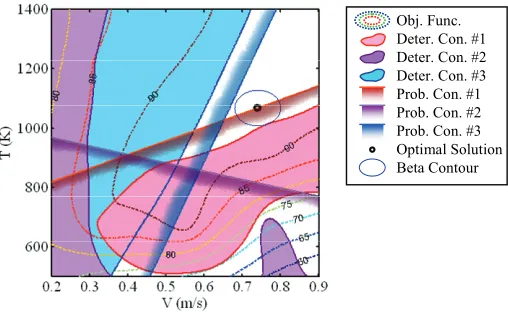
Instead of using the traditional optimization formulations and neglecting the design uncertainties, many Reliability-Based Design Optimization (RBDO) algorithms have been developed to formulate probabilistic constraints while the probability of system failures is subjected to an acceptable level. Under the framework of RBDO, a more conservative design is expected to be determined based on the optimality and the feasibilities of the probabilistic constraints.
General RBDO Formulation:
Consider the random designvariables, X, where the jth random design variable, j