171
Iranian (Iranica) Journal of Energy & Environment
Journal Homepage: www.ijee.net
IJEE an official peer review journal of Babol Noshirvani University of Technology, ISSN:2079-2115
Fabrication and Performance Analysis of a Higher Efficient Dual-Axis Automated
Solar Tracker
M. R. Rahman, M. S. Hossain, S. Shehab Uddin, A. S. M. Ibrahim
Institute of Energy, University of Dhaka, Dhaka, Bangladesh
P A P E R I N F O
Paper history:
Received 28 July 2019
Accepted in revised form 16 September 2019
Keywords:
Dual-Axis Solar Tracker Maximum Power Capture Solar Energy
Power Optimization
A B S T R A C T
In this work, a dual-axis automated solar tracker is developed by using two linear motors, four light dependent resistors (LDRs) and two mono crystalline solar panels. The LDRs are placed on the rotating frame where the solar panels are placed to detect the position of the sun and the controller circuit drives the motors to place the frame towards the sun. The controlling unit has been developed using PLC microcontroller. The motor driver circuit has been designed using a code to align the solar panels to a suitable position so that it is exposed to the maximum amount of solar irradiance. The driver circuit receives data from the LDRs and the microcontroller controls the motors to move the panel along its horizontal and vertical axis. To evaluate the performance of the solar tracker, output power of the solar tracker and an identical set of static solar panels set in an optimum fixed orientation are measured from the open-circuit voltage and the short circuit current for two consecutive days. The output power produced by the automatic solar tracker was consistently higher than that by the static solar panel. The energy gain due to using the automatic solar tracker is at highest in the morning and in the afternoon at almost 40%. The lowest value of energy gain is observed during noon at as low as 1%. The average increase in output throughout the day is 24.09%.
doi: 10.5829/ijee.2019.10.03.02
INTRODUCTION1
The use of solar tracker has become widespread in the photovoltaic (PV) system, as it allows a significant increase in output power that contributes to the overall profitability of solar projects [1, 2]. For fix positioned static solar systems, panels are installed in an optimum tilt angle facing a specific direction, so that it can get maximum direct solar radiation, incident perpendicularly on it throughout the year [3, 4]. Direct solar radiation carries almost 90% of the total energy of the solar radiation [5]. But due to Earth’s rotational and transitional motions, daily and yearly available solar radiation and its incident angle on a static solar panel varies time to time limiting the maximum possible output of the system. Earth’s rotational motion causes succession of days and night and its transitional motion causes seasonal variations [6]. In winter, the sun remains in lower elevation in the sky and is visible for few hours in a day. On the other hand, in summer, the sun travels in an orbit that keeps it in higher elevation and the day length is increased. So, in summer solar radiation falls more perpendicularly on the PV panel that ensures much greater energy efficiency [7]. Besides, in regions near the
*Corresponding Author Email: [email protected] (S. Shehab Uddin)
polar circles, days are longer in summer and shorter in winter, while in other areas closer to the Equator, there are much less variations between the length of nights and days [8]. Thus, daily and annual solar trajectories varies based on the latitude of any location and sun’s position and the angle of incidence of solar radiation continuously changes which critically affects the power production potential of a static solar system [9]. Hence, solar tracker is used to get more direct solar radiation on a solar system that maximizes the output power and improves the overall plant efficiency and profitability.
MATERIALS AND METHODS
The construction of the solar tracker is mainly divided into two parts: hardware and software. The hardware part consists of four light dependent resistors (LDR), two linear motors and solar panels. Whereas in the software part a microcontroller circuit is used with a programming code burnt into it as per the requirements.
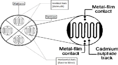
Arrangement of the LDRs
sensor. All four sensors are placed on the same platform along two axes and are separated from each other by a partition. This helps the sensors to avoid any non-uniform or unnatural shadows on any particular sensor [10, 11]. As a result, the LDR sensors register an insolation difference only when there is a considerable variation in the solar radiation readings recorded in the opposite sensors. The intensity of light sensed by the LDRs work as analog input data for the microcontroller [12, 13]. The pair of LDRs installed along the vertical axis (or north-south axis) controls the seasonal tracking of the sun and the pair along the horizontal axis (or east-west axis) dictates the movement along the azimuth. Using this two-axis movement, the solar panel can move freely and follow the path of the sun throughout the day for maximum exposure to sunlight. Figure 1 depicts how the LDRs are arranged in the tracker design.
Designing the driver circuit
In this particular construction, linear motors are used to drive the tracker as opposed to other conventional driving mechanisms. One particular advantage is that a linear motor has a higher natural frequency that allows it to gain higher speed and accuracy [14]. Each of the two linear motors is used for movement on its individual axis. In a linear motor, the stator is unwrapped and laid out flat and the rotor moves in a straight line. As a result instead of producing a torque, a linear motor creates a linear force along its axis. The particular linear motor used in this project requires a supply of 12V DC. One of the two motors moves the tracker along the horizontal axis and is controlled by the pair of LDRs installed on the horizontal axis (Figure 2). The motor responsible for any vertical movement follows the pair of LDRs on the vertical axis (Figure 3). Here, the motors extract power from the solar panel output power to operate. No external power source is required in this case. Hence, all the output measured from the solar tracker excludes the power consumed by the motors and its drive circuit. To avoid any unexpected and faulty movement of the tracker, 10% tolerance is applied on the sensor readings. For less than 10% fluctuation between the values from the LDRs in the similar axis, the tracker does not register an insolation difference and thus does not respond.
Figure 1. Schematic diagram of the LDRs arrangement
Figure 2. Linear motor for horizontal axis movement
Figure 3. Linear motor for vertical axis movement
Flow chart and circuit diagram
The flowchart and circuit diagram of the automated solar tracker are shown in Figures 4 and 5. This flowchart shows how the proposed system assimilates the sensor’s data and operates the driving parts. A programming code is written based on the flowchart. Then the code is converted into a HEX file to burn into the microcontroller. The microcontroller chip used in this experiment is the PIC16F690 which is a low pin count microcontroller. This is a unique microcontroller chip of 20 pin count with a 256 bytes EEPROM data memory and an extended WDT.
Experimental setup
173
Figure 4. Flow chart of dual axis solar tracker
Figure 5. Circuit diagram of dual axis solar tracker
RESULTS AND DISCUSSION
The experimental data reveals that the output voltage and output current and subsequently the output power of the solar panels are dictated by their orientations with respect to the sun.
Observations on day-1: 12 July 2018
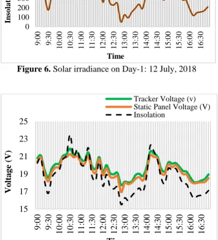
The amount of solar irradiation available at the time of this experiment is shown in Figure 6. From this figure, it
Figure 6. Solar irradiance on Day-1: 12 July, 2018
Figure 7. Comparison for output voltage between static and
dynamic system
higher than the output voltage for the static panels. Also, the highest recorded output voltage for the solar panels accompanied by the tracking system was 21.89 V in contrast with the highest output voltage for the static panels recorded as 21.26 V. The lowest output voltage observed for the tracking systems was 17.74V, which is much higher than the lowest output voltage for the static system as 16.92V. Output Voltage recorded for both systems at noon were at close vicinity although the voltages were not at maximum as expected due to irregular solar insolation which is represented by the dotted line.
Figure 8 represents the comparison between the output currents for the static and the dynamic system. It is seen from the graph that the output current for the automatic solar tracker is always higher than that of the static solar panels. The maximum and minimum output currents for the solar panels associated with the automatic dual axis-tracker was recorded as 1.89A and 0.2A, respectively; in comparison with the output currents recorded for the static panels as 1.56A and 0.2A, respectively.
Figure 8. Output current comparison between static and
dynamic system
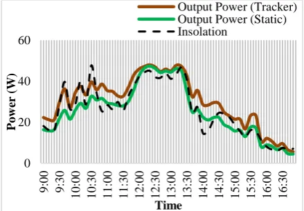
The output currents were lowest around 12:50 pm due to the abrupt change in irradiation caused by the cloudy weather, contradicting the expected highest output values during noon. However, the output values for both the systems were almost the same during noon as the orientation of the panels concerning the sun were in the same at that time. The instantaneous output powers for the static and dynamic systems are illustrated in Figure 9. The behavioral trend of the output powers for both the systems can be easily observed from the graph. The graph represents the comparison between output powers for the static and the dynamic system. The solar panels controlled by the automatic tracking system almost always produce a higher output power than that of the panels with a fixed orientation throughout the day.
For the automatic tracker, the highest power produced was 39.86 Watts at 10:10 am which is almost same as the maximum capacity of the panels i.e. 40 Watts. However, the static panels produced the
Figure 9. Output Power comparison between static and
dynamic system 0 100 200 300 400 500 600 700 800 900 9 :0 0 9 :3 0 1 0 :0 0 1 0 :3 0 1 1 :0 0 1 1 :3 0 1 2 :0 0 1 2 :3 0 1 3 :0 0 1 3 :3 0 1 4 :0 0 1 4 :3 0 1 5 :0 0 1 5 :3 0 1 6 :0 0 1 6 :3 0 In so la ti o n ( W m -2) Time 15 17 19 21 23 25 9 :0 0 9 :3 0 1 0 :0 0 1 0 :3 0 1 1 :0 0 1 1 :3 0 1 2 :0 0 1 2 :3 0 1 3 :0 0 1 3 :3 0 1 4 :0 0 1 4 :3 0 1 5 :0 0 1 5 :3 0 1 6 :0 0 1 6 :3 0 V o lta g e (V ) Time
Tracker Voltage (v) Static Panel Voltage (V) Insolation 0 0.5 1 1.5 2 9 :0 0 9 :3 0 1 0 :0 0 1 0 :3 0 1 1 :0 0 1 1 :3 0 1 2 :0 0 1 2 :3 0 1 3 :0 0 1 3 :3 0 1 4 :0 0 1 4 :3 0 1 5 :0 0 1 5 :3 0 1 6 :0 0 1 6 :3 0 Cu rr en t (I) Time
Tracker Current (A) Static Panel Current (A) Insolation 0 10 20 30 40 50 9 :0 0 9 :3 0 1 0 :0 0 1 0 :3 0 1 1 :0 0 1 1 :3 0 1 2 :0 0 1 2 :3 0 1 3 :0 0 1 3 :3 0 1 4 :0 0 1 4 :3 0 1 5 :0 0 1 5 :3 0 1 6 :0 0 1 6 :3 0 Po w er (W ) Time
175 maximum power at the same time but at a lower value of 32.67 Watts. The lowest output power produced by the static and the dynamic systems were 3.44 and 3.5 Watts, respectively at 12:50 pm when the solar insolation was at its lowest. Although the output power was observed lowest for both the systems at noon, it was almost same for both the systems because the orientation of the automatic solar tracker was similar to the static solar panels facing south at that time.
Observations on day-2: 13 July 2018
The amount of solar irradiation available at the time of this experiment is shown in Figure 10. Figure 11 illustrates the comparison between the output voltages for the static and the dynamic systems. It is evident from the graph that the recorded output voltage for the solar panels with a tracking system is consistently higher than the output voltage for the static panels. The highest recorded output voltage for the solar panels accompanied by the tracking system was 21.55V whereas the highest output voltage for the static panels recorded as 21.34V. The lowest output voltage witnessed for the tracking systems was 19.05V, which is much higher than the lowest output voltage for the static system as 18.04V. Output voltage recorded for two systems at noon were at close vicinity.
Figure 12 reflects the comparison between the output currents for the static and the dynamic systems. It is seen from the graph that the output current for the automatic solar tracker is always higher than that of the static solar panels. The maximum and minimum output currents for the solar panels associated with the automatic dual-axis tracker was recorded as 2.33A and 0.29A, respectively in comparison with the output currents recorded for the static panels as 2.27A and 0.24A respectively. The output currents were highest at 1:30 pm and lowest at around 4:50 pm. The output values for both the systems were almost the same during noon as the orientation of the panels concerning the sun were the same at that time.
The instantaneous output powers for the static and dynamic systems are illustrated in Figure 13. The
Figure 10. Solar irradiation on Day-2: 13th July, 2018
Figure 11. Output voltage comparison between static and
dynamic system
Figure 12. Output current comparison between static and
dynamic system
Figure 13. Output power comparison between static and
dynamic system
behavioral trend of the output powers for both the systems can be easily observed from the graph. The graph represents the comparison between output powers for the static and the dynamic system. The solar panels 0 200 400 600 800 1000 9 :0 0 9 :3 0 1 0 :0 0 1 0 :3 0 1 1 :0 0 1 1 :3 0 1 2 :0 0 1 2 :3 0 1 3 :0 0 1 3 :3 0 1 4 :0 0 1 4 :3 0 1 5 :0 0 1 5 :3 0 1 6 :0 0 1 6 :3 0 In so la tio n (W m -2) Time 15 17 19 21 23 25 9 :0 0 9 :3 0 1 0 :0 0 1 0 :3 0 1 1 :0 0 1 1 :3 0 1 2 :0 0 1 2 :3 0 1 3 :0 0 1 3 :3 0 1 4 :0 0 1 4 :3 0 1 5 :0 0 1 5 :3 0 1 6 :0 0 1 6 :3 0 V o lta g e (V ) Time
Tracker Voltage (v) Static Panel Voltage (V) Insolation 0 0.5 1 1.5 2 2.5 9 :0 0 9 :3 0 1 0 :0 0 1 0 :3 0 1 1 :0 0 1 1 :3 0 1 2 :0 0 1 2 :3 0 1 3 :0 0 1 3 :3 0 1 4 :0 0 1 4 :3 0 1 5 :0 0 1 5 :3 0 1 6 :0 0 1 6 :3 0 Cu rr en t (I) Time
Tracker Current (A) Static Panel Current (A) Insolation 0 20 40 60 9 :0 0 9 :3 0 1 0 :0 0 1 0 :3 0 1 1 :0 0 1 1 :3 0 1 2 :0 0 1 2 :3 0 1 3 :0 0 1 3 :3 0 1 4 :0 0 1 4 :3 0 1 5 :0 0 1 5 :3 0 1 6 :0 0 1 6 :3 0 Po w er (W ) Time
controlled by the automatic tracking system almost always produce a higher output power than that of the panels with a fixed orientation throughout the day. The available solar insolation is represented with a dotted line to get an idea of dependency of output power on the solar irradiance.
For the automatic tracker, the highest power produced was 47.97 Watts at 12:20 pm which is almost the same as the maximum power produced by the static solar panels which was 47.34 Watts at that time. The lowest output power produced by the static and the dynamic systems were 4.48 and 5.63 Watts, respectively at 4:50 pm when the solar insolation was at its lowest. The output power was observed highest for both the system at noon and it was almost same for both the systems because the orientation of the automatic solar tracker was similar to the static solar panels facing south with a significantly small angular difference.
To evaluate the performance of the automatic solar tracker, the increased amount of output power obtained from the panels were calculated comparing with that of the static panels. Figure 14 represents the percentage increase in output power for using an automatic dual-axis solar tracker on 12th July 2018. As it can be seen from the graph, the performance gain of the solar tracker was significantly low during noon whereas it was much higher otherwise. Increase in the output power by using solar tracking systems was observed as high as 23% in the morning and the afternoon and as low as 1% during noon. The average increase in output power throughout the day was calculated to be 14.97%.
The percentage increase in output power by using an automatic dual axis solar tracker on 13th July, 2018 is represented in Figure 15.
The graph illustrates that the energy gain due to using the automatic solar tracker was at highest in the morning and in the afternoon at almost 40%. The lowest value of energy gain was observed during noon at as low as 1%. The average increase in output throughout the day was 24.09%.
Figure 14. Energy gain by using automatic solar tracker
(12th July, 2018).
Figure 15. Energy gain by using automatic solar tracker
(13th July, 2018)
The output power produced by the automatic solar tracker was consistently higher than the power produced by the static solar panel. Energy gain or the percentage increase in the output power was the highest during the morning and the afternoon and the lowest at noon. It can be realized from the position of the static and dynamic systems at noon as they were both facing the same direction with a slight difference in angle. The experiment reveals although that the electrical energy generated by the solar panels is dictated by the availability of solar irradiation, the efficiency of an automatic dual-axis solar tracker always dominates the static system irrespective of the solar insolation.
CONCLUSION
A successful design of an automatic dual axis solar tracker was implemented in construction in this research. The performance analysis further verifies a significant improvement in the performance of the solar panel when assisted with the tracker. A significant increase in output power by exploiting this automatic solar tracker is claimed to be achieved. An even better performance is predicted if exposed to a greater irradiation during summer. This design is constructed using locally available and comparatively cheap materials making it cost effective as opposed to other imported solar trackers.
ACKNOWLEDGEMENT
The authors are thankful to the authority of Institute of Energy, University of Dhaka for the construction of the automatic dual-axis solar tracker in its premises. The authors would also like to thank Professor Dr. Saiful Huque, Director, Institute of Energy, University of Dhaka for his benevolent guidance and support.
0% 5% 10% 15% 20% 25%
9
:0
0
9
:3
0
1
0
:0
0
1
0
:3
0
1
1
:0
0
1
1
:3
0
1
2
:0
0
1
2
:3
0
1
3
:0
0
1
3
:3
0
1
4
:0
0
1
4
:3
0
1
5
:0
0
1
5
:3
0
1
6
:0
0
1
6
:3
0
%
In
cr
ea
se
in
O
u
tp
u
t
Time
0.00% 5.00% 10.00% 15.00% 20.00% 25.00% 30.00% 35.00% 40.00% 45.00%
9
:0
0
9
:3
0
1
0
:0
0
1
0
:3
0
1
1
:0
0
1
1
:3
0
1
2
:0
0
1
2
:3
0
1
3
:0
0
1
3
:3
0
1
4
:0
0
1
4
:3
0
1
5
:0
0
1
5
:3
0
1
6
:0
0
1
6
:3
0
%
In
cr
ea
se
in
O
u
tp
u
t
177
REFERENCES
1. Lee, C.Y., Chou, P.C., Chiang, C.M. and Lin, C.F., 2009. Sun tracking systems: a review. Sensors, 9(5), pp.3875-3890. 2. Sinha, D. and Hui, N.B., 2016. Fuzzy Logic-based Dual Axis
Solar Tracking System. International Journal of Computer Applications, 155(12), pp.13-18.
3. Okhaifoh, J.E. and Okene, D.E., 2016. Design and Implementation of A Microcontroller Based Dual Axis Solar Radiation Tracker. Nigerian Journal of Technology, 35(3), pp.584-592.
4. Xu, X.L. and Zuo, Y.B., 2012. Universal-Joint Sun Tracking Method and Tracking Device. In Advanced Materials Research (Vol. 383), Trans Tech Publications, pp. 3605-3609.
5. Mansouri, A., Krim, F. and Khouni, Z., 2018. Design of prototype dual axis tracker solar panel controlled by geared dc servo motors, pp.1-38.
6. Rhif, A., 2011. A position control review for a photovoltaic system: dual axis sun tracker. IETE technical review, 28(6), pp.479-485.
7. Srinivasa Rao, K., Rajesh, M., Sreedhara Babu, G., (2017). Analysis of automatic sun tracking system with dual axis.
International Journal of Modern Trends in Engineering & Research, 4(6), pp.106-113.
8. Afiqah, N.N., Syafawati, N.A., Idris, S.S.H., Haziah, A.H. and Syahril, M.D., 2015. Development of dual axis solar tracking system performance at Ulu Pauh, Perlis. In Applied Mechanics and Materials (Vol. 793), Trans Tech Publications pp. 328-332. 9. Yu, H.J., Wang, Y.L., Li, J.Y. and He, X.L., 2012. The Design of
Automatic Solar Tracker. In Applied Mechanics and Materials (Vol. 190), Trans Tech Publications, pp. 742-745. 10. Wang, J.M. and Lu, C.L., 2013. Design and implementation of a
sun tracker with a dual-axis single motor for an optical sensor-based photovoltaic system. Sensors, 13(3), pp.3157-3168. 11. Kumar, V.S.S. and Suryanarayana, S., 2014. Automatic dual Axis
sun tracking system using LDR sensor. International Journal of Current Engineering and Technology, 4(5), pp.3214-3217. 12. Chettri, S., Chettri, A., and Chettri, S., (2016). Dual Axis
Self-tracking Solar Panel. International Journal of Computer Applications, 141(14), pp.37-40.
13. Mistri, R.K., Singh, K., Kumar, U., Bharti, P., Kumari, P., (2018). Solar Tracker using LDR. International Journal for Research in Applied Science & Engineering Technology (IJRASET), 6(5), pp.2242-2244.
14. Li, Y.J. and Tien, S.C., 2014. Linear Model‐based Feedforward Control for Improving Tracking‐performance of Linear Motors. Asian Journal of Control, 16(6), pp.1602-1611.