Designing Incomplete Hub Location-routing Network in Urban Transportation Problem

International Journal of Engineering

J o u r n a l H o m e p a g e : w w w . i j e . i r

Designing Incomplete Hub Location-routing Network in Urban Transportation

Problem

M. Setak *_{, H. Karimi, S. Rastani}

Department of Industrial Engineering, K.N.Toosi University of Technology, Tehran, Iran.

P A P E R I N F O

Paper history:

Received 14 March 2013

Received in revised form 15 April 2013 Accepted 18 April 2013

Keywords:

Hub Location Multiple Allocation Valid Inequalities Transportation Network Routing

A B S T R A C T

In this paper, a comprehensive model for hub location-routing problem is proposed which no network structure other than connectivity is imposed on the backbone (i.e. Network between hub nodes) and tributary networks (i.e. Networks which connect non-hub nodes to hub nodes). This model is applied in public transportation, telecommunication and banking networks. In this model locating and routing is considered simultaneously and it has a multiple allocation strategy to allocate non-hub nodes to hub nodes. In addition, non-hub nodes can connect directly to each other. The objective of the proposed model is minimizing costs of establishing a network and transferring flows. To expedite solving the proposed model and improve the lower bound, which gain from linear relaxation, a number of preprocessing tests and valid inequalities are presented which have relatively good performance in the proposed model. Their performance is analyzed by implementing them on the test problems. Results show that using all preprocessing tests and valid inequalities is the best approach to solve the problem among all proposed approaches in this paper.

doi:10.5829/idosi.ije.2013.26.09c.07

1. INTRODUCTION1

Flow of passenger requires a complex connection between origins and destinations. The topology of many to many transportation problems is a significant problem in supply chain network. In this problem, the hub network is designed for servicing people between multiple nodes. Using hubs, a complete network changes to a network with fewer links. Low cost of network construction, flow consolidation and organizing are the advantage of this configuration. Moreover, economies of scale through flows combination are another benefit of using hubs in urban transportation systems.

Originally, the hub location problem was introduced by O’Kelly [1]. Afterwards, he proposed a single allocation hub location quadratic model formulation [2]. The rest of the literature is investigated about closing the formulation of the real-world problems. Other types of hub location consist of hub covering [3], hub center [4] and capacitated hub location problem [5]. Readers

*Corresponding Author Email:[email protected] (M. Setak)

interested in the hub network can read Alumur and Kara [6].

Three assumptions were often considered in the classical hub location: Firstly, the hub network was completely interconnected. Secondly, a discount factor

1

0£a£ was considered in using hub links, and finally, non-hub nodes cannot be directly connected. In the third assumption, direct link between the non-hub nodes is not allowed. These assumptions are relaxed in this research to make close this model to urban transportation problems. Theses relaxations create an incomplete hub network. Incomplete hub network topology generally is categorized into four classes: tree, ring, special, and general shape. Our hub network lies in the fourth category.

Contreras et al. [11] reduced variables and constraints compared with their previous models.

In the ring topology, there is only one cycle in the hub network and each hub node only links with two hubs. There are few researches in this area of hub networks [12]. Lee et al. [13] suggested a single allocation hub-ring model formulation. Additionally, Chiu et al. [14] proposed a ring structure in hub network problems. Finally, Wang et al. [15] suggested a ring shape in the telecommunication systems.

Hub networks are limited by managers, and it is not the same as the ring and tree shapes. For example, a multiple allocation non-linear model that all hubs should be linked only with one hub was introduced by Wasner and Zapfel [16]. Calik et al. [17] presented a model, which transfers flow from a node to another one and at most four hubs can be used. Alumar et al. [18] presented an incomplete hub network over a single allocation p-hub problem. In addition, besides considering the cost of establishing hub nodes, transfer cost is taken into account.

In the general topology, the form of hub network is defined by model and each structure can be created. In this type, there is no condition over the hub network topology. Therefore, we call it as the general form. Yoon et al. [19] proposed a model of a general topology of hub networks, which did not consider the fixed cost of hubs. Moreover, their model included many variables and constraints. Afterwards, Nickel et al. [20] introduced a different model in this area with many variables and constraints. Then, Yoon and Current [21] presented another model without shipping cost. Glareh and Nickel [22] suggested a reduced model of Nickel et al. [20]. They reduced variables and constraints. All papers in the general topology used multiple strategies.

As already stated, the third basic assumption in the hub location area is the lack of direct connection between non-hubs. It was initially relaxed by Aykin [23, 24]. Sung and Jin [25] proposed another model of direct shipment between non-hubs over multiple allocation strategy. In addition, Nickel et al. [20], Yoon and Current [21] and Catanzaro et al. [26] relaxed this assumption.

To the best of our knowledge, in the extensive literature on the hub location problem, the creating (or maintaining) cost of links between non-hubs and hubs are not considered. However, in urban transportation it should be taken into account. With the lack of attention to this cost, models tend to make more spoke links (i.e. a link between a hub node and a non-hub node). Therefore, a new variable is introduced to establish the spoke link. Furthermore, non-hub direct connections are employed. Because, often there exist direct links between some non-hub nodes which can be used in a cheaper way than routing via hubs. In the next section, a new model is proposed.

2. DESCRIPTION OF THE PROBLEM AND MODEL

In this section, the modeling of the problem under the stated conditions is presented, and then some features of the model will be described. It is assumed that the number of input nodes isN. The elements of Nare assumed to represent the origins and destinations and at the same time are potential points for establishing hubs. The aim is to designate some of these nodes as hubs and build a general hub network topology to minimize the total cost included the cost of routing, establishing links between hub nodes, hub node and non-hub nodes, establishing hubs and establishing links between non-hub nodes in the network. Each origin-destination path consists of three or one components. When hubs are used to transshipment, a path contains collections from origin to the first hub, transfer between the first hub and last hub and distribution from the last hub to the destinations. Paths containing only one hub node are also allowed. When hubs are not used in a path, a direct link from origin to destination is employed.

Firstly, parameters and inputs used in the model are introduced. a is assumed as economies of scale, and it uses in inter-hub connections. Transfer cost from node i toj is shown by

c

ij, and the cost graph is non-directional and satisfy the triangle inequality.

w

ij shows the amount of flow transshipment between nodes

i and j. Costs for establishing inter-hub links between nodes m and k is shown byI_km, and Jijis the cost of establishing links between i and j, which at most one of them is the hub. After the introduction of inputs and parameters, variables are introduced. aijkm,eijk, fijk,gij,

ij

b , z_km and y_k are binary variables. The following decision variables are considered:

ï î ï í ì =

0 1

km ij

a

If the flow originated at i and destined at j is routed via hubs k and m

Otherwise

ï î ï í ì =

0 1

ij

b

If non-hub nodes i and j are connected to each other

Otherwise

ï î ï í ì =

0 1

k ij

e

If the flow originated at the non - hub node i

and destined at the node j is routed via a hubk

Otherwise

ï î ï í ì =

0 1

k ij

f

If the flow originated at the node i and destined at non-hub node j is routed via a hub k

ï î ï í ì = 0 1 ij g

If the node i is connected to a node j and just one of them be a hub node

Otherwise ï î ï í ì = 0 1 km z

If hub nodes k and m are connected to each other Otherwise ï î ï í ì = 0 1 k y

If the node k is a hub node

Otherwise

Accordingly, a model for HLRNUTP under incomplete backbone network and direct connections between non-hub nodes is proposed:

åå

å å

å

åå

åå

ååå

åååå

> > + + + + + + + + a

i j i ij ij ij

k m kkmkm

k k k

i j ij ij ij

i j ij ij ij

i j k

k ij kj k ij ik ij km ij

i j k m km ij

b g J z I y F b w c g w c f c e c w a w c ) ( ) ( min (1) 1 = + + å + å ¹

¹ m i ij ij

m ij i

m im

ij e g b

a "i,j,(i¹ j) ₍₂₎

1 = + + å + å ¹

¹ m j ij ij

m ij j

m mj

ij f g b

a _{"i,j,(i¹j) (3)}

0 ,

, + - å + =

å ¹ ¹ m ij k j m mk ij m ij k i m km

ij f a e

a (4) ) , , ( , ,

,jk i ji k j k

i ¹ ¹ ¹

"

i k

ij y

e £1- "i,j,k,(i¹ j) (5)

j k

ij y

f £1- "i,j,k,(i¹ j) (6)

k k j m km ij k

ij a y

e + å £

¹ , "i,j,k,(i¹ j,i¹k,j¹k) (7)

k k i m km ij k

ij a y

f + å £

¹, "i,j,k,(i¹ j,i¹k,j¹k) (8)

j i j i m mj ij j i m im ij ij ij

ij a a a y y

g + + å + å £ +

¹

¹, ,

2

(9)

) ( , ,j i j

i ¹

"

j i

ij y y

g £2- - "i,j,(i¹ j) (10)

j i

ij y y

b £2-

-2 "i,j,(i¹ j) (11)

2 ³ å

kyk (12)

km mk ij km

ij a z

a + £ "i,j,k,m,(i¹ j,k¹m) (13)

ik k

ij g

e £ "i,j,k,(i¹j) (14)

kj k

ij g

f £ "i,j,k,(i¹j) (15)

0 = - _ji

ij b

b "i,j,(i¹ j) (16)

0 = - _ji

ij g

g "i,j,(i¹ j) (17)

0

=

- mk

km z

z "k,m,(k¹m) (18)

0

³

km ij

a "i,j,k,m (19)

0

³

k ij

e "i,j,k (20)

0

³

k ij

f "i,j,k (21)

0 ³ ij

b "i,j (22)

0 ³ ij

g "i,j (23)

{ }

0,1 Î

km

z "k,m (24)

{ }

0,1 Î k

y "k (25)

The objective function (1) minimizes four factors in the network design problem. 1) Minimizing transfer costs, which lies in the first, second, third, and the fourth part of the objective function. 2) Minimizing costs of establishing hubs, which lies in the fifth part of the objective function. 3) Minimizing costs of establishing links between hubs that lies in the sixth part of the objective function. 4) Last part of the objective function minimizes costs of establishing spoke links or two non-hub nodes. Constraints (2) and (4) balance the flow on origins-destination nodes and connections between them, respectively. Constraints (5) and (6) ensure that variables k

ij

e and f_ijk can take values when node i and j are not hubs. Constraints (7) and (8) guarantee if k is a hub, the flow can pass through it to reach the destination. Using an edge for transferring flow from an origin to a destination depends on the roles of origin and destination nodes (being hub nodes or not) that constraints (9) illustrate it. Constraints (10) assure that

ij

Constraints (11) show that if none of the nodes i and j are not a hub, then b_ij can take a value. Constraint (12) guarantees there are at least two hubs. In this case, concept of hubs and use of discount factor makes sense. Constraints (13) ensure that if there is a link between two hubs k and m then a_ijkm or a_ijmk can take a value. Constraints (14) and (15) illustrate that if there is a link between a hub and a non-hub node then it is possible to use this link in non-hub nodes send or receive flows. Constraints (16)-(18) assure that sending path is similar to receiving path because the cost matrix is non-directional. Constraints (19)-(23) guarantee that in the absence of link capacity constraints, flow transfer variables take either zero or one, so there is no need to limit them to binary variables [27]. In the constraints (24) and (25), hub and hub link establishing variables are taken as binary variables. HLRNUTP has

1 2 4

5 3 2

4_{+ n + n - n+}

n constraints, _n4_+2n3_+2n2 non-negative variables and n2+n _{binary variables, while} the model proposed by Nickel et al. [20] has

2 3

4 _{3 5}

2n + n + n constraints _2n4 _{non-negative variables} and n2+n _{binary variables. It shows that the number of} constraints and variables in the HLRNUTPP is lower. This model has two main features that expressed as below:

If constraints (26) are added to the HLRNUTP, it will be a single allocation model:

1 £ å

¹i

j gij "i ( 2 6 )

If constraints (27) are added to the model, the hub network will change to a tree network, because in tree networks the number of hub links is one unit less than the number of nodes. According to the constraints (18), the right side of constraint (27) is multiplied by 2:

å

-= å å

¹ k k

kmk ij

y

z 2 2 _{( 27)}

Accordingly, to the above features, most of existing hub networks, can be produced by using these features. For example, if constraints (26) and (27) are used, the designed network will be similar to models, which Contreras et al. proposed [10, 11]. However, for all origins and destination nodes bij should be zero (

0

=

ij

b ). In the next section, a group of valid inequalities will be presented to tighter the model and improve the lower bound, which gain from linear relaxation.

3. VALID INEQUALITY

In this section, six valid inequalities are presented to cut the solution space, which gain from linear relaxation:

k

km y

z £ "k,m,(k¹m) (28)

m

km y

z £ "k,m,(k¹m) (29)

Proposition 1. Inequalities (28) and (29) are valid for the HLRNUTP.

Proof A link will connect two hubs k and

m

when only both of them are hubs simultaneously. It should be noted that these inequalities were not considered as constraints in the model, because the combination of constraints (5), (9) and (13) satisfy (28) and (29).

å -£ å å

¹

¹ ¹i i j iij

j k j

k

ij N y b

e ( 2)(1 ) _{"i (30)}

å -£ å å

¹

¹ ¹j j i j ij

i k i

k

ij N y b

f ( 2)(1 ) _{"j (31)}

Proposition 2. Inequalities (30) and (31) are valid for the HLRNUTP.

Proof If node i was a non-hub node and was not connected to any other non-hub nodes directly, the maximum amount that _{å å}

¹ ¹i

j k j

k ij

e can take is N-2, becausej¹i, k¹ j and each node can connect to all hub nodes. However, if this node has direct connections to all other non-hub nodes then the number of connections must be subtracted fromN-2. Due to this, the maximum value of the expression is shown in inequalities (30). For the inequalities (31), the same is true.

) (

2 -å

³ å å

¹ k k

i j igij N y (32)

Proposition 3. Inequalities (32) are valid for the HLRNUTP.

Proof As mentioned, gij shows the connection between hub and non-hub node. If the problem is single allocation, the sum of these variables takes its minimum value. So, the number of links is -å

k k y

N that is

exactly equal to the number of non-hub nodes, but according to constraints (17), this value must be doubled.

k k

må¹zkm³y "k (33)

Proof If the node k is hub then due to constraints (2)-(12), it must be linked at least to another hub. In inequalities (33), if

k

was hub, å ³1

¹k m km

z will satisfy.

k k

m km

ij y

a £

å

¹ "i,j,k,(i¹ j) (34)

m m

k km

ij y

a £

å

¹ "i,j,m,(i¹ j) (35)

Proposition 5. Inequalities (34) and (35) are valid for the HLRNUTP.

Proof As the variable aijkm is defined, k and m should be hubs. Therefore, to send flow from origin i to destination jthrough nodes k and m, they must be hubs to send or receive flow through other hubs. This is shown in inequalities (34) and (35).

4. COMPUTATIONAL STUDY

In this section, to simplify the calculations, some preprocessing tests are introduced. Then, performances of the model, preprocessing tests and valid inequalities have been analyzed using the data that presented below. Equations (36)-(38) can process before solving the problem to reduce its computational time.

0 = ii

g "i (36)

0 =

k ik

e "i,k (37)

0 =

k ik

f "i,k (38)

4. 1. Test Data In this section, data from Australia Post (AP), and Civil Aeronautics Board, which is known as CAB is used. CAB data has been proposed by O’Kelly [1] in location literature and it has 25 nodes. Subsets of 5, 10, 15, and 20 of this data are defined in the literature and have been used in this paper. Australia Post has been proposed by Ernst and Krishnamoorthy [28]. In this data, maximum number of nodes is 200 and the flow between these nodes is asymmetric. They described how to generate different problems from 200 nodes. In this paper, the data of 10, 15 and 20 for AP data is used. Because solving large problems takes too longer time than our assumption (4800 seconds), large data have not been analyzed. 0.5, 0.7 and 0.9 are selected fora. Costs of establishing hub nodes for the CAB and AP data are considered 20000000 and 5000, respectively. In addition, I_km=5000c_km, j_ij =3000c_ij are considered for CAB data and Ikm=200ckm, jij=100cij are considered for AP data. In this paper, problems are shown as (data name. number of nodes.10´a). For

example AP. 10. 7 means AP data is used, which has 10 nodes and ais considered 0.7.

4. 2. Performance of Preprocessing Tests and Valid Inequalities In this section, problems are solved in eight different approaches to examine the performance of proposed preprocessing tests and valid inequalities. These approaches are defined as below: 1) Without any preprocessing tests and valid inequalities. 2) Considering preprocessing tests.

3) Considering valid inequalities (28) and (29). 4) Considering valid inequalities (30) and (31). 5) Considering valid inequalities (32). 6) Considering valid inequalities (33). 7) Considering valid inequalities (34) and (35).

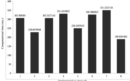
8) Considering all preprocessing tests and valid inequalities. Computational results are shown in Table 1,Table 2 and Table 3. These tables show the performance of the gap between lower bound and optimal solution

(

100´(Obj-LB) LB

)

, computation time and the number of nodes that used in CPLEX 12, respectively. The columns of the tables show the results of these eight approaches. Moreover, for showing the performance of these eight approaches are presented in Figures 1, 2 and 3.

Figure 1. Average difference between lower bound and

optimal solution by using preprocessing tests and valid inequalities

Figure 2. Average computation time using preprocessing tests

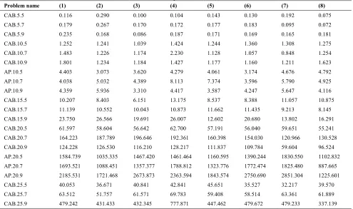
TABLE 1. Distance between lower bound and optimal solution (%)

Problem name Obj (1) (2) (3) (4) (5) (6) (7) (8)

CAB.5.5 181813613.940 8.280 8.280 8.280 3.177 4.218 4.218 1.008 0.142

CAB.5.7 197536151.516 3.341 3.341 1.306 0.354 2.543 2.555 0.910 0.000

CAB.5.9 208846921.664 1.835 1.835 0.501 0.409 0.803 0.803 0.501 0.407

CAB.10.5 552178664.502 2.786 2.786 0.135 0.000 0.518 0.518 0.000 0.000

CAB.10.7 654758680.717 4.893 4.893 0.089 0.000 0.908 0.908 0.000 0.000 CAB.10.9 704606804.884 0.627 0.627 0.039 0.000 0.061 0.061 0.039 0.000

AP.10.5 83070.531 2.147 1.463 1.019 0.969 0.844 1.019 0.948 0.192

AP.10.7 87583.425 3.860 2.896 1.406 1.406 1.327 1.406 1.406 0.534

AP.10.9 90683.985 2.365 1.629 1.222 1.222 1.213 1.117 1.222 0.253

CAB.15.5 1534117270.580 0.152 0.152 0.052 0.000 0.152 0.152 0.000 0.000

CAB.15.7 1953618380.467 0.058 0.058 0.000 0.005 0.058 0.058 0.000 0.000 CAB.15.9 2309141263.790 0.047 0.047 0.047 0.047 0.047 0.047 0.047 0.047 CAB.20.5 3105531710.571 0.028 0.028 0.028 0.028 0.028 0.028 0.023 0.023 CAB.20.7 4094611708.218 0.102 0.102 0.102 0.098 0.102 0.102 0.096 0.096

CAB.20.9 5009268462.858 0.030 0.030 0.000 0.004 0.030 0.030 0.000 0.000

AP.20.5 102310.008 2.300 0.187 0.000 0.000 0.000 0.000 0.000 0.000

AP.20.7 108198.250 4.472 1.953 0.235 0.211 0.235 0.227 0.046 0.046

AP.20.9 113420.332 1.889 1.119 1.045 1.045 1.045 1.045 1.045 0.704

CAB.25.5 4635198134.409 0.000 0.000 0.000 0.000 0.000 0.000 0.000 0.000 CAB.25.7 6233477303.842 0.000 0.000 0.000 0.000 0.000 0.000 0.000 0.000 CAB.25.9 7780980662.224 0.025 0.025 0.025 0.025 0.025 0.025 0.025 0.013

TABLE 2. Computational time (s)

Problem name (1) (2) (3) (4) (5) (6) (7) (8)

CAB.5.5 0.116 0.290 0.100 0.104 0.143 0.130 0.192 0.075

CAB.5.7 0.179 0.267 0.170 0.172 0.177 0.183 0.095 0.072

CAB.5.9 0.235 0.168 0.086 0.187 0.171 0.169 0.165 0.181

CAB.10.5 1.252 1.241 1.039 1.424 1.244 1.360 1.308 1.275

CAB.10.7 1.483 1.226 1.174 2.230 1.128 1.057 0.848 1.254

CAB.10.9 1.801 1.234 1.184 1.427 1.177 1.160 1.211 1.623

AP.10.5 4.403 3.073 3.620 4.279 4.061 3.174 4.676 4.792

AP.10.7 4.038 5.032 4.389 8.113 7.374 3.596 5.790 4.925

AP.10.9 4.359 5.936 3.310 4.417 3.587 4.247 5.647 4.116

CAB.15.5 10.207 8.403 6.151 13.175 8.537 8.388 11.057 10.875

CAB.15.7 11.139 10.552 10.043 10.873 11.662 11.435 9.213 8.145

CAB.15.9 23.750 26.566 19.691 26.007 12.602 20.680 13.802 16.291

CAB.20.5 61.597 58.604 56.642 62.700 57.191 56.040 59.651 55.241

CAB.20.7 164.223 187.789 196.646 192.361 160.398 154.030 120.966 130.528 CAB.20.9 124.228 126.530 116.210 128.217 111.837 109.784 59.604 96.524 AP.20.5 1584.739 1035.335 1467.420 1461.464 1160.595 1390.244 1830.550 1102.832 AP.20.7 1693.521 1088.451 1357.377 1788.812 1323.776 1772.474 1825.480 887.665 AP.20.9 2185.531 1721.468 2673.873 2363.594 1843.574 2750.690 2851.304 1225.601

CAB.25.5 40.053 36.671 40.841 42.841 45.651 35.527 32.217 39.570

CAB.25.7 63.512 51.757 61.571 69.783 59.408 58.514 63.361 61.889

TABLE 4. Results of optimal network structure

Problem name Hub Hub-link Spoke link Link between

non-hub nodes Problem name Hub Hub-link Spoke link

Link between non-hub nodes

CAB.5.5 2 1 4 3 CAB.15.9 6 9 24 7

CAB.5.7 2 1 5 3 CAB.20.5 18 18 36 0

CAB.5.9 2 1 4 1 CAB.20.7 16 38 19 1

CAB.10.5 6 8 8 3 CAB.20.9 11 22 31 4

CAB.10.7 5 5 11 4 AP.20.5 3 2 17 0

CAB.10.9 2 1 11 9 AP.20.7 3 2 19 0

AP.10.5 3 2 9 1 AP.20.9 3 2 20 0

AP.10.7 2 1 9 5 CAB.25.5 24 59 2 0

AP.10.9 2 1 10 4 CAB.25.7 24 63 2 0

CAB.15.5 13 24 13 0 CAB.25.9 15 38 35 3

CAB.15.7 11 23 15 1

TABLE 3. Number of nodes

Problem name (1) (2) (3) (4) (5) (6) (7) (8)

CAB.5.5 1 2 0 0 2 1 0 0

CAB.5.7 5 5 3 0 0 5 0 0

CAB.5.9 0 4 0 4 0 0 3 0

CAB.10.5 0 0 0 0 0 0 0 0

CAB.10.7 0 0 0 0 0 0 0 0

CAB.10.9 0 0 0 0 0 0 0 0

AP.10.5 5 5 7 7 7 3 7 3

AP.10.7 7 7 5 7 7 5 7 3

AP.10.9 5 5 5 5 5 5 5 3

CAB.15.5 0 0 0 0 0 0 0 0

CAB.15.7 0 0 0 0 0 0 0 0

CAB.15.9 5 3 3 5 0 3 3 3

CAB.20.5 0 0 0 0 0 0 0 0

CAB.20.7 3 5 5 3 5 3 3 4

CAB.20.9 0 0 0 0 0 0 0 0

AP.20.5 0 0 0 0 0 0 0 0

AP.20.7 5 3 5 7 3 7 5 3

AP.20.9 9 7 9 9 9 9 9 7

CAB.25.5 0 0 0 0 0 0 0 0

CAB.25.7 0 0 0 0 0 0 0 0

CAB.25.9 0 0 0 0 0 0 0 0

Figure 3. Average number of nodes that used for

implementing different approaches

4. 3. Performance Study Figures 1, 2 and 3 show

that the best approach to solve the problem is using all preprocessing tests and valid inequalities (approach eight). Approach eight’s lower bound is twenty times less than approach one’s. Inequalities (38) and (39) have the most effect on improving lower bound, but these inequalities increase computational times. Approach eight has a 38% improve on computational time compared with approach one. In fact, approach eight solved test problems 1.68 times faster. In addition, CPLEX uses fewer nodes to solve the problem in average.

Table 4 presents the number of hub nodes and links in the optimal solutions. This table shows that as a increases, tendency to establish hub nodes decreases. In this case, with 86% probability, the number of links between non-hub nodes will not reduce. Therefore, managers can analyze the problem based on avalues in terms of the number of hub nodes to decide better. According to Table 2, computational times for two data with 20 nodes are quite different; one reason for this difference is the number of hub nodes in the optimal solution. As the number of hub nodes increases, the computational time decreases.

5. CONCLUSION AND FUTURE WORK

In this study, a comprehensive and flexible model for hub location- routing problems is provided. In addition to its application in the transportation industry, it can also be used in telecommunication networks and banking. To expedite solving the HLRNUTP, a number of preprocessing tests and valid inequalities are presented which have relatively good performance in the HLRNUTP. The contributions of this paper are as follows:

allows establishing direct links between non-hub nodes.

· Despite existing works in the literature, objective function of the HLRNUTP includes the cost of routing, hub location and establishing links between hub nodes, hub node and hub nodes and non-hub nodes.

· A number of valid inequalities presented for model stability, improving lower bound, which obtained from linear relaxation, and decreasing computational time.

It can be concluded that the proposed model is a good approximation for hub location routing problem’s applications in the real world. In addition, using all presented preprocessing tests and valid inequalities decreases computational time and improves lower bound. Future researches could concentrate on hub capacities and connections between hub nodes.

6. ACKNOWLEDGMENTS

The authors would like to thank Professor Vladimir Marianov for his helpful and valuable comments on this model formulation and analysis.

7. REFERENCES

1. O'Kelly, M. E., "The location of interacting hub facilities",

Transportation Science, Vol. 20, No. 2, (1986), 92-106. 2. O'kelly, M. E., "A quadratic integer program for the location of

interacting hub facilities", European Journal of Operational Research, Vol. 32, No. 3, (1987), 393-404.

3. Alumur, S. and Kara, B. Y., "Network hub location problems: The state of the art", European Journal of Operational Research, Vol. 190, No. 1, (2008), 1-21.

4. Karimi, H. and Bashiri, M., "Hub covering location problems with different coverage types", Scientia Iranica, Vol. 18, No. 6, (2011), 1571-1578.

5. Campbell, A. M., Lowe, T. J. and Zhang, L., "The p-hub center allocation problem", European Journal of Operational Research, Vol. 176, No. 2, (2007), 819-835.

6. Correia, I., Nickel, S. and Saldanha-da-Gama, F., "The capacitated single-allocation hub location problem revisited: A note on a classical formulation", European Journal of Operational Research, Vol. 207, No. 1, (2010), 92-96. 7. Kim, J.-G. and Tcha, D.-w., "Optimal design of a two-level

hierarchical network with tree-star configuration", Computers & Industrial Engineering, Vol. 22, No. 3, (1992), 273-281. 8. Lee, Y., Lim, B. H. and Park, J. S., "A hub location problem in

designing digital data service networks: Lagrangian relaxation approach", Location Science, Vol. 4, No. 3, (1996), 185-194. 9. Zhang, L., The tree-hub center allocation proble”m, in 47th

Annual Southeast Regional Conference. Clemson. (2009) 10. Contreras, I., Fernández, E. and Marín, A., "Tight bounds from a

path based formulation for the tree of hub location problem",

Computers & Operations Research, Vol. 36, No. 12, (2009), 3117-3127.

11. Contreras, I., Fernández, E. and Marín, A., "The tree of hubs location problem", European Journal of Operational Research, Vol. 202, No. 2, (2010), 390-400.

12. Klincewicz, J. G., "Hub location in backbone/tributary network design: A review", Location Science, Vol. 6, No. 1, (1998), 307-335.

13. Lee, C.-H., Ro, H.-B. and Tcha, D.-W., "Topological design of a two-level network with ring-star configuration", Computers & Operations Research, Vol. 20, No. 6, (1993), 625-637. 14. Chiu, S., Lee, Y. and Ryan, J., "A steiner ring star problem in

designing survivable telecommunication networks", Informs National Meeting, New Orleans, (1995).

15. Wang, Z., Lin, C. and Chan, C.-K., "Demonstration of a single-fiber self-healing cwdm metro access ring network with unidirectional oadm", Photonics Technology Letters, IEEE, Vol. 18, No. 1, (2006), 163-165.

16. Wasner, M. and Zäpfel, G., "An integrated multi-depot hub-location vehicle routing model for network planning of parcel service", International Journal of Production Economics, Vol. 90, No. 3, (2004), 403-419.

17. Calık, H., Alumur, S. A., Kara, B. Y. and Karasan, O. E., "A tabu-search based heuristic for the hub covering problem over incomplete hub networks", Computers & Operations Research, Vol. 36, No. 12, (2009), 3088-3096.

18. Alumur, S. A., Kara, B. Y. and Karasan, O. E., "The design of single allocation incomplete hub networks", Transportation Research Part B: Methodological, Vol. 43, No. 10, (2009), 936-951.

19. Tcha, D. W., "Optimal design model for a distributed hierarchical network with fixed-charged facilities",

International Journal of Management Science, Vol. 6, No. 2, (2000), 29-45.

20. Nickel, S., Schobel, A. and Sonneborn, T., "Hub location problems in urban traffic networks", Mathematical methods on optimization in transportation systems, Kluwer Academic Publishers, Dordrecht, The Netherlands, (2001), 95-107. 21. Yoon, M.-G. and Current, J., "The hub location and network

design problem with fixed and variable arc costs: Formulation and dual-based solution heuristic", Journal of the Operational Research Society, Vol. 59, No. 1, (2006), 80-89.

22. Gelareh, S. and Nickel, S., "Hub location problems in transportation networks", Transportation Research Part E: Logistics and Transportation Review, Vol. 47, No. 6, (2011), 1092-1111.

23. Aykin, T., "Lagrangian relaxation based approaches to capacitated hub-and-spoke network design problem", European Journal of Operational Research, Vol. 79, No. 3, (1994), 501-523.

24. Aykin, T., "The hub location and routing problem", European Journal of Operational Research, Vol. 83, No. 1, (1995), 200-219.

25. Sung, C. and Jin, H., "Dual-based approach for a hub network design problem under non-restrictive policy", European Journal of Operational Research, Vol. 132, No. 1, (2001), 88-105.

26. Catanzaro, D., Gourdin, E., Labbe, M. and Özsoy, F. A., "A branch-and-cut algorithm for the partitioning-hub location-routing problem", Computers & Operations Research, Vol. 38, No. 2, (2011), 539-549.

27. Campbell, J. F., "Integer programming formulations of discrete hub location problems", European Journal of Operational Research, Vol. 72, No. 2, (1994), 387-405.

28. Ernst, A. T. and Krishnamoorthy, M., "Efficient algorithms for the uncapacitated single allocation p -hub median problem",

Designing Incomplete Hub Location-routing Network in Urban Transportation

Problem

M. Setak, H. Karimi, S. Rastani

Department of Industrial Engineering, K.N.Toosi University of Technology, Tehran, Iran.

P A P E R I N F O

Paper history:

Received 14 March 2013

Received in revised form 15 April 2013 Accepted 18 April 2013

Keywords:

Hub Location Multiple Allocation Valid Inequalities Transportation Network Routing

هﺪﯿﮑﭼ

نﺎﮑﻣﻪﻠﺌﺴﻣياﺮﺑﻊﻣﺎﺟﯽﻟﺪﻣ،ﻪﻟﺎﻘﻣﻦﯾارد

ﯽﺑﺎﯾ

-ﻪﺑﻢﻫﺎﺑطﺎﻘﻧطﺎﺒﺗرازاﺮﯿﻏﻪﺑيرﺎﺘﺧﺎﺳﻪﮐﺖﺳاهﺪﺷﻪﺋارارﻮﺤﻣﯽﺑﺎﯾﺮﯿﺴﻣ

ﺖﺳاهﺪﺸﻧﻞﯿﻤﺤﺗﻪﮑﺒﺷ

.

ﻪﮑﺒﺷردلﺪﻣﻦﯾا

ﻪﮑﺒﺷ،ﯽﻣﻮﻤﻋﻞﻘﻧوﻞﻤﺣيﺎﻫ

ﻪﮑﺒﺷوﯽﺗاﺮﺑﺎﺨﻣيﺎﻫ

دﺮﺑرﺎﮐﯽﮑﻧﺎﺑيﺎﻫ

دراد

.

رد

نﺎﮑﻣﺮﺑهوﻼﻋلﺪﻣﻦﯾا

ﺎﻫرﻮﺤﻣوﺎﻫرﻮﺤﻣﺮﯿﻏﻦﯿﺑلﺎﺼﺗاياﺮﺑﻪﻧﺎﮔﺪﻨﭼﺺﯿﺼﺨﺗيﮋﺗاﺮﺘﺳازا ،نﺎﻣﺰﻤﻫﯽﺑﺎﯾﺮﯿﺴﻣوﯽﺑﺎﯾ

ﻪﺑ

ﺖﺳاهﺪﺷيﺮﯿﮔرﺎﮐ

.

ﯽﻣﻢﻫﺎﻫرﻮﺤﻣﺮﯿﻏﻦﯿﻨﭽﻤﻫ

ﺪﻨﺷﺎﺑﻪﺘﺷادطﺎﺒﺗراﻢﯿﻘﺘﺴﻣرﻮﻃﻪﺑﺪﻨﻧاﻮﺗ

. .

ﻪﻨﯿﻤﮐ،لﺪﻣﻦﯾازافﺪﻫ

يزﺎﺳ

ﻪﻨﯾﺰﻫ

ﻧاوﻪﮑﺒﺷدﺎﺠﯾايﺎﻫ

ﯽﻣﻪﮑﺒﺷردنﺎﯾﺮﺟلﺎﻘﺘ

ﺪﺷﺎﺑ

.

ﯽﻄﺧيزﺎﺳدازآزاﯽﺷﺎﻧﻦﯿﯾﺎﭘﺪﺣدﻮﺒﻬﺑولﺪﻣﻞﺣردﻊﯾﺮﺴﺗﺖﻬﺟ

ﺖﺳاهﺪﺷﻪﺋارا،شزادﺮﭘﺶﯿﭘوﺮﺒﺘﻌﻣيوﺎﺴﻣﺎﻧيداﺪﻌﺗ،لﺪﻣ

.

هدﺎﯿﭘﻪﺑﻪﺟﻮﺗﺎﺑ

نآيزﺎﺳ

ﻪﻠﺌﺴﻣيورﻪﺑﺎﻫ

رددﻮﺟﻮﻣﻪﻧﻮﻤﻧيﺎﻫ

ﺖﺳاﻪﺘﻓﺮﮔراﺮﻗﺶﺠﻨﺳ درﻮﻣنﺎﺷدﺮﮑﻠﻤﻋ،ﻖﯿﻘﺤﺗتﺎﯿﺑدا

.

ﯾﺎﺘﻧ

ﯽﻣنﺎﺸﻧ ﺞ

يوﺎﺴﻣﺎﻧﯽﻣﺎﻤﺗ زاهدﺎﻔﺘﺳا ﻪﮐﺪﻫد

ﺶﯿﭘوﺎﻫ

شزادﺮﭘ

شورﻦﯿﺑردﻞﺣشورﻦﯾﺮﺘﻬﺑﺎﻫ

دﻮﺑﺪﻫاﻮﺧﺶﻫوﮋﭘﻦﯾاهﺪﺷيزﺎﺳهدﺎﯿﭘﺮﮕﯾدﻞﺣيﺎﻫ

.