A Review of Energy Consumption Issues in Various Layers of Protocol Stack in MANET

(1)

Volume 2, Issue 2, 2015

214 Available online at www.ijiere.com

International Journal of Innovative and Emerging

Research in Engineering

e-ISSN: 2394 - 3343

A Review of Mobility Models for Energy Conservation

in Mobile Adhoc Network

Ramanna Havinal

a

_{, Girish V Attimarad}

b

_{and M N Giriprasad}

c a_{M B E Society’s College of Engineering Ambajogai Maharashtra ,India}

b_{Dayanand Sagar College of Engineering Bengaluru, Karnataka, India} c_{J NTUA College of Engineering Anantapuram, Andhra Pradesh, India}

ABSTRACT:

Mobility models are one of the key parameters to consider to analyze the performance of the certain protocol in their simulation environment by the researchers. The mobility model is designed to describe the movement pattern of mobile user and how their location, velocity and acceleration change over time. It is essential to study

and analyze various mobility models and their effect on MANET protocols The selection of mobility model can have a

major impact on the routing scheme and can thus influence performance. We reviewed several mobility models that represent mobile nodes whose movements are independent of each other (i.e. entity mobility models) and several mobility models that represent mobile nodes whose movements are dependent on each other (i.e. group mobility models. The goal of this paper is to present a number of mobility models in order to offer researchers more informed choices when they are deciding on a mobility model to use in their performance evaluations

Keywords: Mobility model , Adhoc network , Trace Models , Synthetic Models , Entity, Group

I. INTRODUCTION

A Mobile Ad hoc Network (MANET) is a collection of wireless nodes communicating with each other in the absence of any infrastructure. The mobility model is designed to describe the movement pattern of mobile users, and how their location, velocity and acceleration change over time. Since mobility patterns may play a significant role in determining the protocol performance. It is desirable for mobility models to emulate the movement pattern of targeted real life applications in a reasonable way. Otherwise, the observations made and the conclusions drawn from the simulation studies may be misleading. Thus, when evaluating MANET protocols, it is necessary to choose the proper underlying mobility model[1]-[4].The mobility patterns are the key criteria that influence the performance characteristics of the mobile ad hoc networks. Many mobility models are designed in order to recreate the real world scenarios better for application to MANET. [1][2]

Mobility impacts all layers of the network protocol stack. At the link layer it determines how fast the link characteristics change and whether or not the link connectivity is stable over time. At the medium access control (MAC) layer it affects how long measurements regarding channel and interference conditions remain in effect and how scheduling algorithms perform. At the network layer mobility has major implications for the performance of different routing protocols. The impact of mobility on network performance ultimately dictates which applications can be supported on a highly mobile network. The impact of mobility on ad hoc wireless network design will be discussed in more detail throughout the article. Generally, there are two types of mobility models 1.Trace based mobility models and 2. Synthetic mobility models

(2)

215 In reality, the performance of mobile ad hoc networks will depend on many factors such as node mobility model, traffic pattern, network topology, radio interference, obstacle positions, and so on. It is difficult to cover all these factors in simulation study of ad hoc routing protocols. However, it has been shown that mobility pattern plays an important role in performance of ad hoc routing protocols. The same protocol can perform very differently in different mobility patterns. Random Waypoint[1]-[4]represents typical random node movement pattern but could be unrealistic in many real situations. A few different mobility models have been developed to model different ad hoc network environments other than entirely random movements .A mobility model should attempt to mimic the movements of real MNs. Changes in speed and direction must occur and they must occur in reasonable time slots. This survey gives insight into the most recent trades and evolution of mobility models, highlighting operation. The survey also gives insight into the applicability of mobility models, beyond the common simulation application environment

II. RELATED WORK

Bai et al. [1] provide a categorization of mobility models (both individual and group) splitting them into four main groups according to their main feature, namely, randomness capability, temporal correlation, spatial correlation, geographic constraint. Camp et al. [2] provide another categorization for mobility models in ad-hoc networking, by splitting them into two main groups: entity and group mobility models. In addition to the categorization the authors provide a performance evaluation concerning the impact of the different models on multihop routing, showing that the choice of a mobility model can have a significant effect on their performance. Jianli Zhao et.al in[6] provides A formula to calculate the connectivity probability of mobile ad hoc network was proposed, the relationship among the number of nodes, the range of nodes and the connectivity probability .

III. NOTION AND TERMIMALOGY

A node is denoted as a wireless enabled device integrating at least one interface. Node position describes the specific location of a node . The mobility features that capture a node movement in mobility models are a node’s speed and also a direction. For some specific models, another feature considered is node’s acceleration. The pause time of a node relates to the time period that a node is steady in a specific position, i.e., the interval of time when the node’s speed is zero or close to zero. Inter-contact time corresponds to the time interval between two consecutive contacts of the same two nodes. As for contact duration, this refers to the time period two nodes attain while within the same radio range . 3.1 Mobility Models

The mobility model plays a very important role in determining the protocol performance in MANET. Thus, it is essential to study and analyze various mobility models and their effect on MANET protocols. The mobility model is designed to describe the movement pattern of mobile users, and how their location, velocity and acceleration change over time. Since mobility patterns may play a significant role in determining the protocol performance, it is desirable for mobility models to emulate the movement pattern of targeted real life applications in a reasonable way. Thus, when evaluating MANET protocols, it is necessary to choose the proper underlying mobility model. Mobility models are based on setting out different parameters related to node movement. Basic parameters are the starting location of mobile nodes, their movement direction,velocity range, speed changes over time. Figure 1 illustrates Types of mobility models[1]

Figure 1 Types of mobility models[1]

One intuitive method to create realistic mobility patterns would be to construct trace-based mobility models, in which accurate information about the mobility traces of users could be provided. However, since MANETs have not been implemented and deployed on a wide scale, obtaining real mobility traces becomes a major challenge. Therefore, various researchers proposed different kinds of mobility models, attempting to capture various characteristics of mobility and represent mobility in a somewhat 'realistic' fashion. Much of the current research has focused on the so-called synthetic mobility models [2] that are not trace-driven. However, to model and analyze the mobility models in MANET, the movement of individual nodes at the microscopic-level, including node location and velocity relative to other nodes are to be considered, because these factors directly determine when the links are formed and broken since communication is peer-to-peer[1]. Figure types of mobility model.

3.2 Mobility Categories

(3)

216 Random models: In Random models like statistical models, nodes move randomly and can be classified further based on the statistical properties of randomness, and random waypoint, random direction, and random walk mobility model fall into this category. In random-based mobility models, the mobile nodes move randomly and freely without restrictions. To be more specific, the destination, speed and direction are all chosen randomly and independently of other nodes. This kind of model has been used in many simulation studies. One frequently used mobility model, the Random Waypoint model, the two variants of the Random Waypoint model, namely the Random Walk model and the Random Direction model,

Temporal dependency Models: It is a measure of how current velocity (magnitude and direction) are related to previous velocity. Nodes having same velocity have high temporal dependency The movement patterns of the mobility models with temporal dependency are likely to be influenced by their movement histories, and Gauss–Markov and smooth random mobility model are the examples of this mobility model category.

Spatial dependency Model: In some mobility scenarios, the mobile nodes tend to travel in a correlated manner. It is a measure of how two nodes are dependent in their motion. If two nodes are moving in same direction then they have high spatial dependency. These mobility models are termed as mobility models with spatial dependency, and mobility models like reference point group mobility model and other spatially correlated mobility models belong to this category.

Geographical restrictions models:In this mobility model the movements of the mobile nodes are constrained by streets, freeways, and/or obstacles, and pathway and obstacle mobility model are two examples of this mobility model . In most real life applications, we observe that a node’s movement is subject to the environment. In particular, the motions of vehicles are bounded to the freeways or local streets in the urban area, and on campus the pedestrians may be blocked by the buildings and other obstacles. Therefore, the nodes may move in a pseudo-random way on predefined pathways in the simulation field. Some recent works address this characteristic and integrate the paths and obstacles into mobility models.

3.3 Mobility Metrics

The mobility metrics aim to capture the characteristics of different mobility patterns and can be used to analyze the impact of mobility models on the performance of communications protocols used over mobile ad hoc networks. The metrics should also, if possible, be independent of the particular network technology used. Many mobility models can be used in mobile ad hoc networks, and each mobility model has its own mobility patterns that will impact the protocol performances. Each mobility model will also behave differently when there are obstructions. But models themselves do not give clear images of how mobility patterns are different from each other. The mobility metrics that describe these mobility patterns will be termed as the direct mobility metrics[5].

The parameters for the direct mobility metrics are considered as follows: relative velocity, temporal dependence, spatial dependence, and pause time. The direct mobility metrics will then be used to find the derived mobility metrics using some mathematical models primarily representing the generic network performances: mobility measure, link-based metrics, path-based metrics, node connectivity, network connectivity, and quality of service. The combined metrics are then termed as the mobility performance metrics for the mobile ad hoc network. The direct mobility metrics measure the speed and direction-related parameters of the mobile node directly. The direct mobility metrics are used to measure different mobility models successfully, although some metrics cannot accurately capture different characteristics of mobility models. For example, the metric indicates the degree of mobility, but it fails to reflect relative motions between hosts. More important, direct mobility metrics often do not directly reflect topology changes, while the latter is believed to be more influential to network performance. The derived mobility metrics take care of this aspect of mobility and constitute precise mathematical relationships between network connectivity and node mobility. These expressions can, therefore, be employed in a number of ways to compare the different mobility models. In turn, it will improve the performance of mobile ad hoc networks such as in the development of efficient algorithms for communications protocols.

3.4 Mobility Patterns

A mobility model attempts to mimic the movement of real mobile nodes that change the speed and direction with time. The mobility model that accurately represents the characteristics of the mobile nodes in an ad hoc network is the key to examine whether a given protocol is useful in a particular type of mobile scenario[2]. The possible approaches for modeling of the mobility patterns are of two types: traces and syntactic.

3.4.1 Trace Models

For predicting stability of the nodes, movement patterns history and monitoring on periodic movements is required. Movement pattern of nodes provide path of mobile node which maintains degree of stability in the network. In the literature authors have concluded that stability of nodes can be enhanced by predicting future position of nodes. The traces provide those mobility patterns that are observed in real-life systems. In trace-based models, everything is deterministic. However, mobile adhoc networks are yet to be deployed widely to know the traces involving a large number of participants and an appropriately long observation period[2].

3.4.2 Synthetic Models:

(4)

217 syntactic mobility models can also be classified based on the description of the mobility patterns in ad hoc networks: individual mobile movements and group mobile movements[2].

In the former case, mobility models attempt to anticipate mobile’s traversing patterns from one place to another at a given point of time under various network scenarios. In the latter case, mobility models try to characterize the group’s traversing patterns with individualism averaged. Unlike trace-based mobility models, syntactic mobility models have randomness, and further classifications can be made based on randomness: constrained topology-based models and statistical models. In constrained topology-based mobility models, mobile nodes have only partial randomness where the movement of nodes is restricted by obstacles, pathways, speed limits, and others. If the nodes are allowed to move anywhere in the area and the speed and direction are allowed to choose, it is termed as total randomness. The model that is based on total randomness is defined as statistical mobility model[2]. In statistical mobility model, mobile nodes have total randomness where nodes are allowed to move anywhere in the area and the speed and direction are allowed to choose. The synthetic mobility models attempt to present the movement of entities based on random walking. In these models, nodes can move freely in the simulation area at a randomly chosen speed. The trajectories of movements are straight lines towards each destination ignoring the influence of the environment. These mobility models are the most commonly utilized and can be classified in to entity mobility models and group mobility models based on whether clusters of nodes moving together

IV. CLASSIFICATION OF MOBILITY MODELS

There are two types of MANET mobility models: single entity and group. In individual mobility model, the mobility pattern of the individual mobile node is considered, and random walk is an example of this mobility model In single-entity models, each MN moves independently of all the other MNs within the network area. A characteristic feature of every mobility model is to ensure that a MN will not travel outside the network area. In group mobility models, nodes are assumed to be organized in groups and the mobility of a node is often reflective of the movement pattern of the entire group[5][6][7].

Figure 2. Entity based mobility models[5]

Figure 2 provides a global perspective on the existing individual mobility models, highlighting whether they are synthetic or trace-based, or a mix of both. The details of the models provide a good resource to researchers when they are deciding upon a mobility model to use in their performance evaluations.

1. Random Walk Mobility Model

In this models node movements are independent of each other. Individual mobility modelling attempts to mimic the mobility pattern behavior of a specific node and from a temporal timeframe, were the first type of mobility models. Main features considered in these models are the speed and direction at random and without any restriction, in particular restrictions due to the relation with and to other nodes. Individual mobility modelling attempts to mimic the mobility pattern behavior of a specific node and from a temporal timeframe, were the first type of mobility models. Main features considered in these models are the speed and direction at random and without any restriction, in particular restrictions due to the relation with and to other nodes.The most popular types of individual mobility models are based upon Brownian movement modelling, but more recently, there is an attempt, based on traces, to derive models that better capture movement of individual nodes.

2. Random Walk Mobility Model

(5)

218 Figure 3. Traveling pattern of an MN using the 2-D Random Walk Mobility Model [3]

If an MN that moves according to this model reaches a simulation boundary, it ‘bounces’ off the simulation border with an angle determined by the incoming direction. The MN then continues along this new path. Many derivatives of the Random Walk Mobility Model have been developed including the 1-D, 2-D, 3-D and d-D walks.

Conclusion: The Random Walk Mobility Model with a small input parameter (distance or time) produces Brownian motion and, therefore, basically evaluates a static network, when used in a performance investigation. A large input parameter (distance or time) is similar to the Random Waypoint Mobility Model without pause times. The main difference between these two mobility models is that MNs are more likely to cluster in the center of the simulation area with the Random Waypoint Mobility Model. The Random Walk Mobility Model is a memoryless mobility pattern because it retains no knowledge concerning its past locations and speed values [1][4]. The current speed and direction of an MN is independent of its past speed and direction [3][5]. This characteristic can generate unrealistic movements such as sudden stops and sharp turns.

3. Random Waypoint Mobility Model

This model is widely used by the researchers. It generates non homogenous spatial distribution of nodes. It contains both feature of entity and statistical models.The Random Waypoint Model was first proposed by Johnson and Maltz[5].Because of its simplicity and wide availability, it became a 'benchmark' mobility model to evaluate the MANET routing protocols. In this mobility model as the simulation starts, each mobile node randomly selects one location in the simulation field as the destination. It then travels towards this destination with constant velocity chosen uniformly and randomly from [0,Vmax], where the parameter Vmax is the maximum allowable velocity for every mobile node[6]. The velocity and direction of a node are chosen independently of other nodes. Upon reaching the destination, the node stops for a duration defined by the ‘pause time’ parameter. If pause time is zero, this leads to continuous mobility. After this duration, it again chooses another random destination in the simulation field and moves towards it. The whole process is repeated again and again until the simulation ends.

Figure 4: Traveling pattern of an MN using the Random Waypoint Mobility Model[3]

Figure 4 shows an example traveling pattern of an MN using the Random Waypoint Mobility Model starting at a randomly chosen point. We note that the movement pattern of an MN using the Random Waypoint Mobility Model is similar to the Random Walk Mobility Model if pause time is zero and [0, MAXSPEED] = [speedmin, speedmax][2][3]. Velocity and pause time are two important parameters used in this model. Topology of adhoc network is stable in low velocity and long pause time where as topology is high dynamic if velocity is high and pause time is short. So, by varying these parameters, we can generate various mobility scenarios with different levels of node speed[4][5].

(6)

219 4. Random Direction mobility model

The Random Direction mobility model is a model where the node has the capability to walk near the border of the simulation area, and in contrast to the Random Waypoint , which has a high probability to choose the target in the center of the simulation area.In this model the target is chosen near the boundary of the simulation area. When a node reaches the boundary of the simulation area, it stops for a period and then chooses a new direction by applying an angle between 0 and 1800_{degrees and then resuming movement based on random Walk. By applying this angle, this model prevents} that nodes cross the boundary of the simulation area, given that the direction is limited.

The Random Direction Mobility Model [2]-[7] was created to overcome density waves in the average number of neighbors produced by the Random Waypoint Mobility Model. A density wave is the clustering of nodes in one part of the simulation area. In the case of the Random Waypoint Mobility Model, this clustering occurs near the center of the simulation area. In the Random Waypoint Mobility Model, the probability of an MN choosing a new destination that is located in the center of the simulation area or a destination that requires travel through the middle of the simulation area, is high. Thus, the MNs appear to converge, disperse and converge again.

.

Figure 5a. Traveling pattern of an MN using the Random Direction Mobility Model[3]

Figure 5 shows an example about the random direction model behavior, where a node starts its movement in the center of the simulation area and the direction is changed only if it reaches the boundary of the simulation area. In the random direction model a user chooses a direction to travel in, a speed at which to travel, and time duration for this travel. The Random Direction Mobility Model is an unrealistic model because it is unlikely that people would spread themselves evenly throughout an area (a building or a city). In addition, it is unlikely that people will only pause at the edge of a given area.

Limitations of the Random Waypoint Model and other Random Models:

The Random Waypoint model and its variants are designed to mimic the movement of mobile nodes in a simplified way. Because of its simplicity of implementation and analysis, they are widely accepted. However, they may not adequately capture certain mobility characteristics of some realistic scenarios, including temporal dependency, spatial dependency and geographic restriction :

Temporal Dependency of Velocity: In Random Waypoint and other random models, the velocity of mobile node is a memoryless random process, i.e., the velocity at current epoch is independent of the previous epoch. Thus, some extreme mobility behavior, such as sudden stop, sudden acceleration and sharp turn, may frequently occur in the trace generated by the Random Waypoint model. However, in many real life scenarios, the speed of vehicles and pedestrians will accelerate incrementally. In addition, the direction change is also smooth.

Spatial Dependency of Velocity: In Random Waypoint and other random models, the mobile node is considered as an entity that moves independently of other nodes. This kind of mobility model is classified as entity mobility model [2]. However, in some scenarios including battlefield communication and museum touring, the movement pattern of a mobile node may be influenced by certain specific 'leader' node in its neighborhood. Hence, the mobility of various nodes is indeed correlated.

Geographic Restrictions of Movement: In Random Waypoint and other random models, the mobile nodes can move freely within simulation field without any restrictions. However, in many realistic cases, especially for the applications used in urban areas, the movement of a mobile node may be bounded by obstacles, buildings, streets or freeways.Random Waypoint model and its variants fail to represent some mobility characteristics likely to exist in Mobile Ad Hoc networks..

5. Gauss Markov Mobility Model

The Gauss-Markov Mobility Model [Figure 5] is a widely used model was first introduced by Liang and Haas . In this model, the velocity of mobile node is assumed to be correlated over time and modeled as a Gauss-Markov stochastic process. When the node is going to travel beyond the boundaries of the simulation field, the direction of movement is forced to flip 180 degree. This way, the nodes remain away from the boundary of simulation field.

(7)

220 Figure 5b. Track of nodes in Gausss Markov Model[2]

This model [4][5] was designed to maintain different levels of randomness by using one varying parameter alpha in mobility pattern. This pattern is based on statistical mobility pattern .and overcome the problem of sudden changes in random waypoint mobility model. At each fixed intervals of time n a movement occurs by modifying the speed and direction of node. Value of alpha is lies between 0 and 1. If it is zero then brownian motion is obtained otherwise linear motion is obtained. By varying the value of alpha [0, 1], intermediate levels of randomness could be obtained. Value of next location is calculated based on current location

6.

Boundless simulation area

In this model, speed and direction of each node is changing rapidly. At every regular time, node adjusts its direction and speed by doing changes in current values of these two parameters direction and speed. In this model, nodes move in unobstructed way in the simulation boundary. As a result, it converts 2D rectangular area into torous shaped simulated area. This Mobility Model provides movement patterns that one might expect in the real world.

Figure 6 : Travelling Pattern of Boundless simulation area Mobility model

In addition, this model is the only one that allows MNs to travel unobstructed in the simulation area, thus removing any simulation edge effects from the performance evaluation. One concern, however, is the undesired side effects that would occur from allowing the MNs to move around a torus. For example, one static MN and one MN that continues to move in the same direction become neighbors again and again. In addition, a simulation area without edges would force modification of the radio propagation model to wrap transmissions from one edge of the area to the other. Figure 6 illustrates the Travelling Pattern of Boundless simulation area Mobility model

7. Manhattan Model

The Manhattan mobility model [1]-[5] uses a grid road topology. This model is mainly proposed for the movement in urban area, where the streets are in an organized manner and the mobile nodes are allowed to move only in horizontal or vertical direction. At each intersection of a horizontal and a vertical street, the mobile node can turn left, right or go straight with certain probability. Like the City Section model, each MN is initially placed on a random street intersection, but the Manhattan model utilizes a probabilistic approach for movement on the streets. The movement of a node is decided one street at a time. To start with, each node has equal chance (i.e., probability) of choosing any of the streets leading from its initial location. After a node begins to move in the chosen direction and reaches the next street intersection, the subsequent street in which the node will move is chosen probabilistically. If a node can continue to move in the same direction or can also change directions, then the node has 50% chance of continuing in the same direction, 25% chance of turning to the east/north and 25% chance of turning to the west/south, depending on the direction of the previous movement. If a node has only two options, then the node has an equal (50%) chance of exploring either of the two options. If a node has only one option to move (this occurs when the node reaches any of the four corners of the network), then the node has no other choice except to explore that option.

(8)

221 .

Figure 7. Topography showing the movements of nodes for Manhattan Mobility model[5]

However, when the node A arrives to position (3,2), it has four choices to change direction, i.e., it can change direction with a 25% probability, as said previously. In this case it choose the right side and goes to position (3,3). Usually, each interception area provides an opportunity for a node choose one of four side to move. It is important emphasize that in Manhattan mobility model, a node’s velocity is always limited by the velocity of the node preceding it on the same lane of the street. This model can be used in Mobile Ad-hoc Networks (MANET) and Vehicular Ad-hoc Networks (VANET) simulators.

8. Probabilistic version of Random Walk

The Probabilistic Random Walk mobility model[1]-[3] considers a set of probabilities to determine the next position of a node. For this, the model considers a matrix which keeps the node’s current position (state 0), the node’s previous position (state 1), and the node’s next position (state 2). Figure 8 provides an operational example on how this model works, showing a matrix for the different states of a node’s movement assuming as starting position A and as potential next positions B, C, and D. For instance, the node has 0.2 probability of staying on the same position, while it has 0.3 probability of moving from A to B, and 0.4 of moving from A to C. However, its first movement will be to D, which has 0.2 probability

0.2 0.3 0.4 0.2

0.2 0.5 0.1 0.3

0.3 0.1

0.4 0.3

0.2 0.1

0.5 0.6

Figure 8. Matrix for node position

While the Probabilistic Random Walk Mobility Model also provides movement patterns that one might expect in the real world, choosing appropriate parameters for the probability matrix may be difficult. This model could become useful, however, when we have scenario trace data that we want to model. Although this model has other ways to define the previous or next movement of a mobile node, it inherits the main features of Random Walk and hence does not capture realistic node behavior of nodes in mobile wireless networks [6].

4 City Section Mobility Model

The city section model [6[[7] provides realistic movements for nodes located within specific city sections, by restricting to polar coordinates the traveling behavior of mobile nodes. Nodes are initially randomly placed in street intersections (Figure 9). Each street is then associated with a specific speed limit, and with a length (e.g. one side of a square block). These two parameters give the means to determine the time it takes to move in the street. Initially, each MN is randomly placed on an intersection. A MN then moves to another randomly chosen intersection with at most one vertical and one horizontal motion. This movement is also the shortest path between the two street intersections

Figure 9. City Section mobility model scenario[5]

Each MN continues to move to randomly chosen street intersections until the simulation time is reached. Nodes then choose a random target street intersection where they are going to move. The path followed by the node between its current and chosen location corresponds to a shortest-path in terms of travelling time. When the node reaches its target, a pause time can be considered, after which the process is repeated. The city section model is a model frequently applied in Vehicular adhoc Networks (VANETs).

(9)

222 a city, since it severely restricts the traveling behavior of MNs; MNs do not have the ability to roam freely without regard to obstacles and other traffic regulations. Further development of this model (e.g. to use realistic city maps) is desired.

5 Model-T

The mobility model T (Model-T) 3]-[5] is based on traces that relate to user registration in APs of a specific campus. Their authors extensively analyzed traces and extracted features that were common, such as: the user registration patterns are highly skewed in space distributions; and the spatial distribution of user registration patterns is hierarchical. Such features were then analyzed and correlated to both time and space and a probabilistic model was derived. Model-T assumes that there are specific positions where nodes cluster forming communities of nodes being a node’s movement based on probabilities between these clusters and also intra-cluster. In addition to the fine-grained possibility of considering both inter and intra-cluster mobility aspects, Model-T also considers a number of metrics to determine the movement of mobile nodes, such as node popularity, the average of incoming transitions for all nodes in a cluster.

V. GROUP MOBILITY MODELS

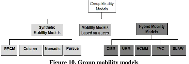
In this model [Figure10][5] mobile nodes movement dependent of one another. The coordination among nodes are formed from the same group. The cooperative group movement of the mobile nodes acts in synchrony as a group. Moreover, in some targeted MANET applications including disaster relief and battlefield, team collaboration among users exists and the users are likely to follow the team leader. Therefore, the mobility of mobile node could be influenced by other neighboring nodes. Figure 10 illustrates types of Group mobility models

Figure 10. Group mobility models

Since the velocities of different nodes are 'correlated' in space, thus we call this characteristic as the Spatial Dependency of velocity

1. Reference Point Group Mobility Model (RPGM)

RPGM model[2]–[4] is based on reference velocity in mobile adhoc network. In this model, each node moves in the group. Reference Point Group Mobility (RPGM) model nodes are divided into groups. In this model, each group has a center, which is either a logical center or a group leader node. We assume that the center is the group leader. Thus, each group is composed of one leader and a number of members. The movement of the group leader determines the mobility behavior of the entire group.

.

Figure 11. Movement of nodes Reference point group mobility model

The leader’s mobility follows random way point the members of the group follow the leader’s mobility closely, with some deviation. At each instant of time, every node has a speed and direction that is specified by randomly deviating from that of the group leader. This general description of group mobility can be used to create a variety of models for different kinds of mobility applications such as conferences, meetings Emergency crews, rescue teams, Military divisions/platoons. It is used as generic method for handling group mobility. The input parameters of the RPGM model allow the flexibility to implement the Column, Nomadic Community, and Pursue Mobility Models.

Figure 11 depicts the movement of two RPs which are, respectively, the RP for a first set of three nodes, and a second set of two nodes (black dots). In Figure 8 the RPs move to a new position and the nodes move based in a position of their RP at the next instant in time. Both the movement of the logical center of each group and the random motion of each individual node within the group is implemented relying on the Random Waypoint mobility model.

(10)

223 needs to be specified to handle both the movement of a group of MNs and the movement of the individual MNs within the group.The input parameters of the RPGM model allow the flexibility to implement the Column, Nomadic Community and Pursue Mobility Models.

2.

Column Mobility

This mobility model attempts to capture a set of mobile nodes that move in the same direction and normally in a straight line as shown in Figure 12. Originally, it was developed to model the movement of a row of robots moving in the same direction (e.g., watering machines in a field).In this model[3][4], center movement is defined as movement of group behavior in terms of velocity, speed, position, direction and acceleration The movement direction is based on a random distance and a random angle .In this mobility model, each node (black dots) has a single reference point (RP) and moves around its reference point via an entity mobility model [2]. The reference point is chosen periodically based on an advance vector, where the new reference point is the sum between the old reference point (the node’s previous reference point) and the advance vector (a predefined offset that moves the reference grid). Additional examples for the applicability of this model are mine searching, or nodes searching for obstacles.

Figure 12. Column mobility model example.[5]

This mobility model can be used in searching and scanning activity, such as destroying mines by military robots When the mobile node is about to travel beyond the boundary of a simulation field, the movement direction is then flipped 180 degree. Thus, the mobile node is able to move towards the center of simulation field in the new direction[6].

3. Pursue Mobility Model

The Pursue Mobility Model [Figure 13] emulates scenarios where several nodes attempt to capture single mobile node ahead. This mobility model can be used in target tracking and law enforcement. The node being pursued (target node) moves freely according to the Random Waypoint model by directing the velocity towards the position of the targeted node, the pursuer nodes (seeker nodes) try to intercept the target node[6]

Figure 13. Pursue mobility model example, two sets of nodes moving towards the same target.[5]

In the Pursue mobility model a reference point is pursued by the other nodes in the group, and the direction, speed and the other parameters of the mobile nodes of this groups are based on the movement of the reference point that being pursued. The new position of each mobile node is determined by the sum of the old position, the acceleration (target - old-position), which is provided on the movement of the reference point being pursued and the random vector, which is a random offset for each mobile node [6]. As shown in Figure 13, we can see nodes (black points) in a group pursuing reference points (white points) to the target; an important feature this model is that the amount of randomness for each mobile node is limited in order to maintain effective tracking of the reference point being pursued [6].

An applicability scenario for this model is a tour guide, where several people have a single guide (RP), and thus the group pursues the tourist guide. This model [2]-[5] is used for target tracking. Consequently, mobile nodes track a particular target. The current position of mobile node is evaluated by adding old position of node and accelerated value of old position with random vector. The value of random vector is calculated by an entity mobility model. Initially, location of target node is stored at position (x1, y1).Then verify all the number of nodes and register location of pursuing node P(x2, y2). If distance of pursuing node is less than distance of target node then evaluate current position of the node otherwise target node is being tracked by pursuing node .

4.

Nomadic Community Mode

]

(11)

224 location to another. Then, the reference point of each node is determined based on the general movement of this group. Figure 14. Provides Nomadic mobility model,

Figure 14. Nomadic mobility model, nodes moving and gravitating towards their RP.[5]

Inside of this group, each node can offset some random vector to its predefined reference point. Being based on the RPGM model, nodes still gravitate around a reference point. The movement of mobile nodes that roam around a given RP is based on a mobility pattern, such as the Random Waypoint mobility model. Applications of the nomadic model include military operations, as well as robotics applied to agriculture. This model could be applied in mobile communication in a conference or military application.

Compared to the Column Mobility Model which also relies on the reference grid, it is observed in [2] that the Nomadic Community Mobility Model shares the same reference grid while in Column Mobility Model each column has its own reference point. Moreover, the movement in the Nomadic Community Model is sporadic while the movement is more or less constant in Column Mobility Model. The Column, Nomadic Community and Pursue Mobility Models are useful group mobility models for specific realistic scenarios. The movement patterns provided by these three mobility models can be obtained by changing the parameters associated with the Reference Point Group Mobility Model

5. Community Based mobility model

The Community based mobility model (CMM) [28] captures a group of nodes in movement in a way that mimics social behavior of nodes. Nodes are grouped into communities. An example of a community is a family, or affiliation.

Figure15. Example of initial node community placement for CMMs[5].

The CMM movement is modeled based upon a “social attractiveness” function. In other words, nodes move towards other nodes and other communities based upon probabilities and taking into account the strength of social associations between nodes. Movement of nodes therefore exhibits a behavior close to the human social behavior.

Figure 15 provides an example of a social network, which is a weighted graph, which represents the strength of social ties between the nodes. In this model the authors use the same value to represent the interaction between two nodes, i.e., it is assumed that the social strength between a node i and j equals the social strength between node j and i. For instance, the interaction between the nodes A and B is 0.8 and the interaction between B and A is the same value (0.8). Hence, the authors’ assumption is that the weight used to express the strength of social ties [35], can also be used as a measure of the likelihood of geographic co-location, i.e., people who share strong social ties tend to move to similar places.

Figure 16. Initial scenario CMM.

(12)

225

VI. CONCLUSION

We observe that the each mobility models may have various properties and exhibit different mobility characteristics. As a consequence, these mobility models behave differently and influence the protocol performance in different ways. Therefore, to thoroughly evaluate ad hoc protocol performance, it is imperative to use a rich set of mobility models. Hence, a method to choose a suitable set of mobility models is needed. The performance of an ad hoc network protocol can vary significantly with different mobility models. The performance of an ad hoc network protocol can vary significantly when the same mobility model is used with different parameters. The selection of a mobility model may require a data traffic pattern which significantly influences protocol performance. The performance of an ad hoc network protocol should be evaluated with the mobility model that most closely matches the expected real-world scenario. the expected real-world scenario is unknown, then researchers should make an informed choice about the mobility model to user. From the study it is observed that no single model is best amongst all, as each has better performance over the other at a particular environment.

VII. REFERENCES

[1] Fan Bai and Ahmed Hellmey : A Survey of mobility models in wireless adhoc networks

[2] T. Camp, J. Boleng, and V. Davies, “A Survey of Mobility Models for Ad Hoc Network Research,” in Wireless Communication & Mobile Computing (WCMC): Special issue on Mobile Ad Hoc Networking: Research, Trends and Applications, vol. 2, no. 5, pp. 483-502, 2002.

[3] Tracy Camp Jeff Boleng Vanessa Davies “ A Survey of Mobility Models for Ad Hoc Network Research. Dept. of Math. and Computer Sciences Colorado School of Mines, Golden, CO

[4] Fabrice Theoleyre, Rabih Tout, Fabrice Valois “New metrics to evaluate mobility models properties "International Symposium on Wireless Pervasive Computing, San Juan P orto Rico”

[5] Andréa G. Ribeiro, Rute Sofia, “A Survey on Mobility Models for Wireless Networks “ SITI Technical Report SITI-TR-11-01February 2011

[6] Jianli Zhao, Xiaofei Jiang, Jing Sha, “A Study of the Relationship between Mobility Model of Ad Hoc Network and Its Connectivity” Journal of Computer Network Vol. 9, No. 4, April 2014

[7] Said EL KAFHALI, Abdelkrim HAQIQ “Effect of Mobility and Traffic Models on the Energy Consumption in MANET Routing Protocols” International Journal of Soft Computing and Engineering (IJSCE) ISSN: 2231-2307, Volume-3, Issue-1, March 2013

[8] R.R. Roy, “Handbook of Mobile Ad Hoc Networks for Mobility Model” Springer

Ramanna Havinal received his B.E, M.E degree from Karnataka University, Dharwad, Indai India in 1991, 2000 respectively. Currently he is pursuing his Ph.D from J N T University Anantapur, India He is having more than 22 years of teaching experience. Presently he is working as Associate Professor in the department of Electronics and Communication Engineering at College of Engineering Ambajogai, Maharashtra, India. His research areas are Wireless Communications, Wireless Networks, Digital signal and Image processing. He has presented more than 15 papers in national and international conferences. He is a life member of ISTE .

Girish V Attimarad received his B.E degree in 1993 from Gulbarga University, India, M.E degree in 1995 from Karnataka University, Dharwad, India and Ph.D degree in 2003 from Delhi University Delhi, India. He is having more than 21 years of teaching experience. Presently he is working as Professor and Head of the department of Electronics and Communication Engineering at Dayanand Sagar College of Engineering, Bengaluru Karnataka, India. His research areas are Wireless Communications, Wireless Networks, Microwaves and Radar, Open wave guides. He has published many papers in national and international journals. He is a life member of ISTE,IE,IETE