The use of iterative methods for solving Black-Scholes equation

Int. J.IndustrialMathematics (ISSN 2008-5621) Vol. 5, No. 1, 2013 Article ID IJIM-00329, 11 pages

Research Article

The use of iterative methods for solving Black-Scholes equation

T. Allahviranloo

∗ †

, Sh. S. Behzadi

‡

————————————————————————————————–

Abstract

In this paper, the Black-Scholes equation is solved by using the Adomian’s decomposition method , modified Adomian’s decomposition method , variational iteration method , modified variational iteration method, ho-motopy perturbation method, modified hoho-motopy perturbation method and hoho-motopy analysis method. The existence and uniqueness of the solution and convergence of the proposed methods are proved in details. A numerical example is studied to demonstrate the accuracy of the presented methods.

Keywords: Black-Scholes equation; Adomian decomposition method (ADM); Modified Adomian decomposition method (MADM); Variational iteration method (VIM); Modified variational iteration method (MVIM); Ho-motopy perturbation method (HPM); Modified hoHo-motopy perturbation method (MHPM); HoHo-motopy analysis method (HAM).

—————————————————————————————————–

1

Introduction

T

he pricing of options is a central problem in

fi-nancial investment. It is of both theoretical and practical importance since the use of options thrives in the financial market. In option pricing theory, the Black-Scholes equation is one of the most effective models for pricing options. The equation assumes the existence of perfect capital markets and the security prices are log normally distributed or, equivalently, the log-returns are normally distributed. To these, one adds the assumptions that trading in all secu-rities is continuous and that the distribution of the rates of return is stationary. In recent years, some works have been done in order to find the numerical solution of the Black-Scholes equation. For example [5,6,7,8,9,10]. In this work, we develope the ADM, MADM, VIM, MVIM, HPM, MHPM and HAM to solve this equation as follows [1,2, 3,4]:

ut+ax2uxx+bxux−ru= 0, (1.1)

where,

a= σ

2, b=r−δ,

∗_{Department of Mathematics, Central Tehran Branch,}

Is-lamic Azad University, Tehran, Iran.

†_{Corresponding author. [email protected]}

‡_{Department of Mathematics, Qazvin Branch, Islamic Azad}

University, Qazvin, Iran.

r is the risk-free rate, σ is the volatility, andδ is the dividend yield. With the initial condition:

u(x,0) =g(x). (1.2)

The paper is organized as follows. In Section 2, the mentioned iterative methods are introduced for solv-ing Eq. 1.1. In Section 3 we prove the existence , uniqueness of the solution and convergence of the proposed methods. Finally, the numerical example is shown in Section4. In order to obtain an approximate solution of Eq. 1.1, let us integrate one time Eq. 1.1

with respect totusing the initial condition we obtain,

u(x, t) =g(x)− (1.3)

a∫₀tF1(u(x, τ)dτ−b∫₀tF2(u(x, τ))dτ+r∫₀tu(x, τ)dτ,

where,

F1(u(x, t)) =x2uxx(x, t),

F2(u(x, t)) =xux(x, t).

In Eq. 1.3, we assumeg(x) is bounded for allxinJ = [0, T](T ∈R). The terms F1(u(x, t)) andF2(u(x, t))

are Lipschitz continuous with|F1(u)−F1(u∗)|≤L1| u−u∗|and|F2(u)−F2(u∗)|≤L2|u−u∗|.

2

The iterative methods

2.1

Description of the MADM and

ADM

The Adomian decomposition method is applied to the following general nonlinear equation

Lu+Ru+N u=f, (2.4)

whereu(x, t) is the unknown function,Lis the highest order derivative operator which is assumed to be easily invertible, R is a linear differential operator of order less than L, N u represents the nonlinear terms, and

f is the source term. Applying the inverse operator

L−1 _{to both sides of Eq. 2.4, and using the given}

conditions we obtain

u(x, t) =z(x)−L−1(Ru)−L−1(N u), (2.5)

where the function z(x) represents the terms arising from integrating the source term f. The nonlinear operatorN u=G1(u) is decomposed as

G1(u) =

∞

∑

n=0

An, (2.6)

whereAn, n≥0 are the Adomian polynomials

deter-mined formally as follows :

An =

1

n![

dn

dλn[N(

∞

∑

i=0

λiui)]]λ=0. (2.7)

The first Adomian polynomials (introduced in [11,12,

13]) are:

A0=G1(u0), A1=u1G′1(u0),

A2=u2G′1(u0) +

1 2!u

2

1G′′1(u0), (2.8)

A3=u3G′1(u0) +u1u2G′′1(u0) +

1 3!u

3

1G′′′1(u0), ...

2.1.1 Adomian decomposition method

The standard decomposition technique represents the solution ofu(x, t) in2.4as the following series,

u(x, t) =

∞

∑

i=0

ui(x, t), (2.9)

where, the componentsu0, u1, . . . which can be

deter-mined recursively

u0(x, t) =g(x), (2.10)

u1(x, t) =−a

∫ t

0

A0(x, t)dt−b

∫ t

0

B0(x, t)dt

+r

∫ t

0

u0(x, t)dt,

.. .

un+1(x, t) =−a

∫ t

0

An(x, t)dt−b

∫ t

0

Bn(x, t)dt

+r

∫ t

0

un(x, t)dt, n≥0.

Substituting2.8 into 2.10leads to the determination of the components ofu.

2.1.2 The modified Adomian decomposition method

The modified decomposition method was introduced by Wazwaz [14]. The modified forms was established on the assumption that the function g(x) can be di-vided into two parts, namely g1(x) andg2(x). Under this assumption we set

g(x) =g1(x) +g2(x). (2.11)

Accordingly, a slight variation was proposed only on the componentsu0 and u1. The suggestion was that

only the partg1be assigned to the zeroth component u0, whereas the remaining part g2 be combined with

the other terms given in 2.11 to define u1.

Conse-quently, the modified recursive relation

u0=g1(x), (2.12)

u1=g2(x)−L−1(Ru0)−L−1(A0),

.. .

un+1=−L−1(Run)−L−1(An), n≥1,

was developed. To obtain the approximation solution of Eq. 1.1, according to the MADM, we can write the iterative formula2.12as follows:

u0=g1(x), (2.13)

u1=g2(x)−a

∫ t

0

A0(x, t)dt−b

∫ t

0

B0(x, t)dt

+r

∫ t

0

u0(x, t)dt,

.. .

un+1=−a

∫ t

0

An(x, t)dt−b

∫ t

0

Bn(x, t)dt

+r

∫ t

0

un(x, t)dt, n≥1.

The operators Fi(u(x, t)) (i= 1,2) are usually

repre-sented by the infinite series of the Adomian polyno-mials as follows:

F1(u) =

∞

∑

F2(u) =

∞

∑

i=0 Bi.

whereAi andBiare the Adomian polynomials. Also,

we can use the following formula for the Adomian polynomials [15]:

An=F1(sn)−

∑n−1

i=0 Ai,

Bn =F2(sn)−

∑n−1

i=0 Bi.

(2.14)

Wheresn=

∑n

i=0ui(x, t) is the partial sum.

2.2

Description

of

the

VIM

and

MVIM

In the VIM [16,17,18,19,20,35,41,42], it has been considered the following nonlinear differential equa-tion:

Lu+N u=g, (2.15) whereLis a linear operator,Nis a nonlinear operator andgis a known analytical function. In this case, the functionsun may be determined recursively by

un+1(x, t) =un(x, t)+ (2.16)

∫ t

0

λ(x, τ){L(un(x, τ)) +N(un(x, τ))−g(x, τ)}dτ,

n≥0,

whereλis a general Lagrange multiplier which can be computed using the variational theory. Here the func-tion un(x, τ) is a restricted variations which means

δun = 0. Therefore, we first determine the Lagrange

multiplier λ that will be identified optimally via in-tegration by parts. The successive approximation

un(x, t), n ≥0 of the solution u(x, t) will be readily

obtained upon using the obtained Lagrange multiplier and by using any selective function u0. The zeroth approximation u0 may be selected any function that just satisfies at least the initial and boundary condi-tions. Withλdetermined, then several approximation

un(x, t),n≥0 follow immediately. Consequently, the

exact solution may be obtained by using

u(x, t) = lim

n_→∞un(x, t). (2.17)

The VIM has been shown to solve effectively, eas-ily and accurately a large class of nonlinear problems with approximations converge rapidly to accurate so-lutions. To obtain the approximation solution of Eq.

1.1, according to the VIM, we can write iteration for-mula2.16as follows:

un+1(x, t) = (2.18)

un(x, t) +L−t1(λ[un(x, t)−g(x) +a

∫ t

0

F1(un(x, t))dt

+b

∫ t

0

F2(un(x, t))dt−r

∫ t

0

un(x, t)dt]), n≥0.

Where,

L−_t1(.) =

∫ t

0

(.)dτ.

To find the optimal λ, we proceed as

δun+1(x, t) = (2.19)

δun(x, t)+δL−t1(λ[un(x, t)−g(x)+a

∫ t

0

F1(un(x, t))dt

b

∫ t

0

F2(un(x, t))dt−r

∫ t

0

un(x, t)dt]).

From Eq. 2.19, the stationary conditions can be obtained as follows: λ′ = 0 and 1 +λ= 0. Therefore, the Lagrange multipliers can be identified as λ=−1 and by substituting in 2.18, the following iteration formula is obtained.

u0(x, t) =g(x), (2.20)

un+1(x, t) =

un(x, t)−L−t1(un(x, t)−g(x) +a

∫ t

0

F1(un(x, t))dt

+b

∫ t

0

F2(un(x, t))dt−r

∫ t

0

un(x, t)dt), n≥0.

To obtain the approximation solution of Eq. 1.1, based on the MVIM [21, 22, 23], we can write the following iteration formula:

u0(x, t) =g(x), (2.21)

un+1(x, t) =

un(x, t)−L−t1(a

∫ t

0

F1(un(x, t)−un−1(x, t))dt

+b

∫ t

0

F2(un(x, t)−un₋1(x, t))dt

−r

∫ t

0

(un(x, t)−un−1(x, t))dt), n≥0.

Relations 2.20 and 2.21 will enable us to determine the componentsun(x, t) recursively forn≥0.

2.3

Description of the HAM

Consider

N[u] = 0,

whereN is a nonlinear operator,u(x, t) is an unknown function andxis an independent variable. letu0(x, t)

denote an initial guess of the exact solution u(x, t),

h̸= 0 an auxiliary parameter,H1(x, t)̸= 0 an

auxil-iary function, andLan auxiliary linear operator with the propertyL[s(x, t)] = 0 whens(x, t) = 0. Then us-ingq∈[0,1] as an embedding parameter, we construct a homotopy as follows:

(1−q)L[ϕ(x, t;q)−u0(x, t)]−qhH1(x, t)N[ϕ(x, t;q)] =

ˆ

H[ϕ(x, t;q);u0(x, t), H1(x, t), h, q].

It should be emphasized that we have great freedom to choose the initial guessu0(x, t), the auxiliary linear operator L, the non-zero auxiliary parameter h, and the auxiliary function H1(x, t). Enforcing the homo-topy2.22to be zero, i.e.,

ˆ

H1[ϕ(x, t;q);u0(x, t), H1(x, t), h, q] = 0, (2.23)

we have the so-called zero-order deformation equation

(1−q)L[ϕ(x, t;q)−u0(x, t)] =qhH1(x, t)N[ϕ(x, t;q)].

(2.24) When q = 0, the zero-order deformation Eq. 2.24

becomes

ϕ(x; 0) =u0(x, t), (2.25) and when q = 1, since h ̸= 0 andH1(x, t) ̸= 0, the zero-order deformation Eq. 2.24is equivalent to

ϕ(x, t; 1) =u(x, t). (2.26)

Thus, according to 2.25 and 2.26, as the embedding parameter q increases from 0 to 1, ϕ(x, t;q) varies continuously from the initial approximation u0(x, t) to the exact solution u(x, t). Such a kind of con-tinuous variation is called deformation in homotopy [23,24,25,26,40]. Due to Taylor’s theorem,ϕ(x, t;q) can be expanded in a power series ofqas follows

ϕ(x, t;q) =u0(x, t) +

∞

∑

m=1

um(x, t)qm, (2.27)

where,

um(x, t) =

1

m!

∂mϕ(x, t;q)

∂qm |q=0.

Let the initial guess u0(x, t), the auxiliary linear pa-rameterL, the nonzero auxiliary parameterhand the auxiliary functionH1(x, t) be properly chosen so that the power series2.27of ϕ(x, t;q) converges at q= 1, then, we have under these assumptions the solution series

u(x, t) =ϕ(x, t; 1) =u0(x, t) +

∞

∑

m=1

um(x, t). (2.28)

From Eq. 2.27, we can write Eq. 2.24as follows

(1−q)L[ϕ(x, t, q)−u0(x, t)] (2.29)

= (1−q)L[

∞

∑

m=1

um(x, t)qm] =q h H1(x, t)N[ϕ(x, t, q)]

⇒L[

∞

∑

m=1

um(x, t)qm]−q L[

∞

∑

m=1

um(x, t)qm]

=q h H1(x, t)N[ϕ(x, t, q)]

By differentiating2.29m times with respect toq, we obtain

{L[

∞

∑

m=1

um(x, t)qm]−q L[

∞

∑

m=1

um(x, t)qm]}(m)=

{q h H1(x, t)N[ϕ(x, t, q)]}(m)=

m! L[um(x, t)−um−1(x, t)] =

h H1(x, t)m ∂

m−1_{N[ϕ(x, t;q)]} ∂qm−1 |q=0 .

Therefore,

L[um(x, t)−χmum−1(x, t)] = (2.30)

hH1(x, t)ℜm(um₋1(x, t)),

where,

ℜm(um−1(x, t)) =

1 (m−1)!

∂m−1_{N[ϕ(x, t;q)]} ∂qm−1 |q=0,

(2.31) and

χm=

{

0, m≤1 1, m >1

Note that the high-order deformation Eq. 2.30

is governing the linear operator L, and the term

ℜm(um₋1(x, t)) can be expressed simply by 2.31 for

any nonlinear operatorN. To obtain the approxima-tion soluapproxima-tion of Eq. 1.1, according to HAM, let

N[u(x, t)] =u(x, t)−g(x)+

a

∫ t

0

F1(u(x, t))dt+b

∫ t

0

F2(u(x, t))dt−r

∫ t

0

u(x, t)dt,

so,

ℜm(um−1(x, t)) =um−1(x, t)−g(x)+

a

∫ t

0

F1(um₋1(x, t))dt+b

∫ t

0

F2(um₋1(x, t))dt

(2.32)

−r

∫ t

0

um−1(x, t)dt.

Substituting2.32into 2.30

L[um(x, t)−χmum₋1(x, t)] =hH1(x, t)[um₋1(x, t)

(2.33)

+a

∫ t

0

F1(um−1(x, t))dt+b

∫ t

0

F2(um−1(x, t))dt

−r

∫ t

0

um₋1(x, t)dt+ (1−χm)g(x)(x)].

We take an initial guess u0(x, t) = g(x), an auxiliary linear operatorLu=u, a nonzero auxiliary parameter

h=−1, and auxiliary function H1(x, t) = 1. This is substituted into2.33to give the recurrence relation

u0(x, t) =g(x),

un+1(x, t) =−a

∫t

0F1(un(x, t))dt

−b

∫ t

0

F2(un(x, t))dt+r

∫ t

0

un(x, t)dt, n≥0.

Therefore, the solutionu(x, t) becomes

u(x, t) =

∞

∑

n=0

un(x, t) =g(x)+ (2.35)

∞

∑

n=1

(

−a

∫ t

0

F1(un(x, t))dt−b

∫ t

0

F2(un(x, t))dt

+r

∫ t

0

un(x, t)dt.

Which is the method of successive approximations. If

|un(x, t)|<1,

then the series solution2.35convergence uniformly.

2.4

Description

of

the

HPM

and

MHPM

To explain HPM [27,28,34,36,37,38,39], we consider the following general nonlinear differential equation:

Lu+N u=f(u), (2.36)

with initial conditions

u(x,0) =f(x).

According to HPM, we construct a homotopy which satisfies the following relation

H(u, p) =Lu−Lv0+p Lv0+p[N u−f(u)] = 0, (2.37)

where p∈[0,1] is an embedding parameter andv0 is an arbitrary initial approximation satisfying the given initial conditions. In HPM, the solution of Eq. 2.37is expressed as

u(x, t) =u0(x, t) +p u1(x, t) +p2 u2(x, t) +... (2.38)

Hence the approximate solution of Eq. 2.36 can be expressed as a series of the power ofp, i.e.

u= lim

p→1u=u0+u1+u2+...

where,

u0(x, t) =g(x),

.. .

um(x, t) = m_∑−1

k=0 −a

∫ t

0

F1(um−k−1(x, t))dt− (2.39)

b

∫ t

0

F2(um−k−1(x, t))dt+r

∫ t

0

um−k−1(x, t)dt,

m≥1.

To explain MHPM [30,31,32], we consider Eq. 1.1as

L(u) =u(x, t)−g(x) +a

∫ t

0

F1(u(x, t))dt+

b

∫ t

0

F2(u(x, t))dt−r

∫ t

0

u(x, t)dt.

Where F1(u(x, t)) = g1(x)h1(t) and F2(u(x, t)) =

g2(x)h2(t). We can define homotopyH(u, p, m) by

H(u,0, m) =f(u), H(u,1, m) =L(u),

where, mis an unknown real number and

f(u(x, t)) =u(x, t)−z(x, t).

Typically we may choose a convex homotopy by

H(u, p, m) =

(1−p)f(u) +p L(u) +p(1−p)[m(g1(x) +g2(x))] = 0,

(2.40) 0≤p≤1.

Where m is called the accelerating parameters, and for m = 0 we define H(u, p,0) = H(u, p), which is the standard HPM. The convex homotopy 2.40

continuously trace an implicity defined curve from a starting point H(u(x, t)−f(u),0, m) to a solution functionH(u(x, t),1, m).The embedding parameterp

monotonically increase from 0 to 1 as trivial problem

f(u) = 0 is continuously deformed to original problem

L(u) = 0. The MHPM uses the homotopy parameter

pas an expanding parameter to obtain

v=

∞

∑

n=0

pnun, (2.41)

whenp→1, Eq. 2.37corresponds to the original one and Eq. 2.41becomes the approximate solution of Eq.

1.1, i.e.,

u= lim

p_→1v=

∞

∑

m=0 um.

Where,

u0(x, t) =g(x),

u1(x, t) =−a∫₀tF1(u0(x, t))dt−b∫₀tF2(u0(x, t))dt

+r∫₀tu0(x, t)dt−m(g1(x) +g2(x)),

u2(x, t) =−a

∫t

0F1(u1(x, t))dt−b

∫t

0F2(u1(x, t))dt

+r∫₀tu1(x, t)dt+m(g1(x) +g2(x)),

.. .

um(x, t) =

∑m−1

k=0 −a

∫t

0F1(um−k−1(x, t))dt −b∫₀tF2(um−k−1(x, t))dt+r

∫t

0um−k−1(x, t)dt, m≥3.

(2.42)

3

Existence and convergency of

iterative methods

We set,

β1:= 1−T(1−α1), γ1:= 1−T α1.

Theorem 3.1 Let 0 < α1 < 1, then Black-Scholes equation 1.1, has a unique solution.

Proof. Letuandu∗ be two different solutions of1.3

then

|u−u∗|=| −a∫₀t[F1(u(x, t))−F1(u∗(x, t))]dt

−b∫₀t[F2(u(x, t))−F2(u∗(x, t))]dt

+r∫₀t[u(x, t)−u∗(x, t)]dt|

≤|a|∫₀t|F1(u(x, t))−F1(u∗(x, t))| dt+

|b|∫₀t|F2(u(x, t))−F2(u∗(x, t))| dt+

|r|∫₀t|u(x, t)−u∗(x, t)| dt≤

T(|a|L1+|b|L2+|r|) |u−u∗|=α1|u−u∗|.

From which we get (1−α1) | u−u∗ |≤ 0. Since

0 < α1 <1, then |u−u∗ |= 0. Implies u=u∗ and

completes the proof. 2

Theorem 3.2 The series solution u(x, t) =

∑_∞

i=0ui(x, t) of problem 1.1 using MADM

con-vergence when0< α1<1,|u1(x, t)|<∞.

Proof. Denote as (C[J],∥ . ∥) the Banach space of all continuous functions on J with the norm

∥ g(t) ∥= max| g(t)|, for all t in J. Define the se-quence of partial sumssn, letsn andsmbe arbitrary

partial sums withn≥m. We are going to prove that

sn is a Cauchy sequence in this Banach space:

∥sn−sm∥=

max_∀t_∈J |sn−sm|=max_∀t_∈J| n

∑

i=m+1

ui(x, t)|=

max_∀t_∈J | −a

∫ t

0

(

n₋1

∑

i=m

Ai)dt−b

∫ t

0

(

n₋1

∑

i=m

Bi)dt+

r

∫ t

0

(

n₋1

∑

i=m

ui)dt|.

From [15], we have

∑n−1

i=mAi=F1(sn−1)−F1(sm−1),

∑n−1

i=mBi=F2(sn−1)−F2(sm−1),

∑n₋1

i=mui= (sn₋1)−(sm₋1).

So,

∥sn−sm∥=max_∀t_∈J| −a

∫t

0[F1(sn−1)−F1(sm−1)]dt −b

∫ t

0

[F2(sn₋1)−F2(sm₋1)]dt

+r

∫ t

0

[(sn₋1)−(sm₋1)]dt|≤|a|

∫ t

0

|F1(sn₋1)

−F1(sm−1)|dt+|b|

∫ t

0

|F2(sn−1)−F2(sm−1)|dt

+|r|

∫ t

0

|(sn₋1)−(sm₋1)| dt≤α1∥sn−sm∥.

Letn=m+ 1, then

∥sn−sm∥≤α1∥sm−sm−1∥≤

α2₁∥sm−1−sm−2∥≤...≤αm1 ∥s1−s0∥.

From the triangle inquality we have

∥sn−sm∥≤∥sm+1−sm∥+∥sm+2−sm+1∥+...+

∥sn−sn₋1∥≤[αm1 +α

m+1

1 +...+α

n−m−1

1 ]∥s1−s0∥ ≤αm₁[1 +α1+α21+...+α

n−m−1

1 ]∥s1−s0∥

≤αm₁ [1−α

n₋m

1

1−α1 ]∥u1(x, t)∥.

Since 0< α1<1, we have (1−αn1−m)<1, then

∥sn−sm∥≤

αm

1

1−α1max∀t∈J|u1(x, t)|. (3.43)

But|u1(x, t)|<∞, so, asm→ ∞, then∥sn−sm∥→

0. We conclude thatsnis a Cauchy sequence inC[J],

therefore the series is convergence and the proof is complete. 2

Theorem 3.3 The maximum absolute truncation er-ror of the series solution u(x, t) = ∑∞_i=0ui(x, t) to

problem1.1by using MADM is estimated to be

max|u(x, t)−

m

∑

i=0

ui(x, t)|≤

kαm₁

1−α1. (3.44)

Proof. From inequality 3.43, when n → ∞, then

sn→uand

max|u1(x, t)|≤T(|a|max∀t∈J|F1(u0(x, t))|+

|b|max_∀t|F2(u0(x, t))|+|r|max∀t∈J |u0(x, t)|).

Therefore,

∥u(x, t)−sm∥≤ α

m

1

1₋α1T(|a|max∀t∈J |F1(u0(x, t))|

+|b|max_∀t|F2(u0(x, t))|+|r|max∀t|u0(x, t)|).

Finally the maximum absolute truncation error in the intervalJ is obtained by3.44.

Theorem 3.4 The solution un(x, t) obtained from

the relation 2.20 using VIM converges to the exact solution of the problem 1.1 when 0 < α1 < 1 and

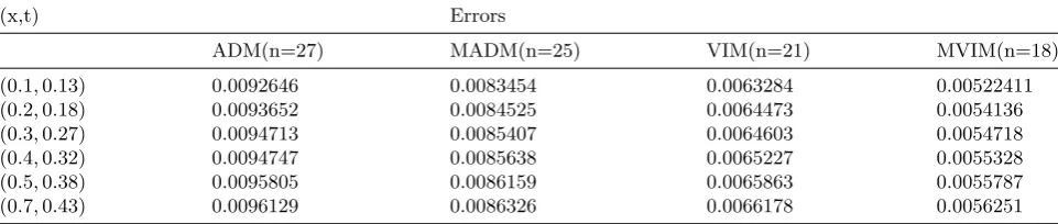
Table 1: Numerical results for Example4.1

(x,t) Errors

ADM(n=27) MADM(n=25) VIM(n=21) MVIM(n=18)

(0.1,0.13) 0.0092646 0.0083454 0.0063284 0.00522411

(0.2,0.18) 0.0093652 0.0084525 0.0064473 0.0054136

(0.3,0.27) 0.0094713 0.0085407 0.0064603 0.0054718

(0.4,0.32) 0.0094747 0.0085638 0.0065227 0.0055328

(0.5,0.38) 0.0095805 0.0086159 0.0065863 0.0055787

(0.7,0.43) 0.0096129 0.0086326 0.0066178 0.0056251

(Continue Table1).

(x,t) Errors

HPM(n=22) MHPM(n=19) HAM(n=14)

(0.1,0.13) 0.0073609 0.0054283 0.0044536

(0.2,0.18) 0.0074447 0.0055081 0.0045475

(0.3,0.27) 0.0075226 0.0056205 0.0046231

(0.4,0.32) 0.0075656 0.0056738 0.0046815

(0.5,0.38) 0.0076267 0.0057048 0.0047462

(0.7,0.43) 0.0076926 0.0057659 0.0047826

Proof.

(3.45)

un+1(x, t) =un(x, t)−Lt−1([un(x, t)−g(x)

+a

∫ t

0

F1(un(x, t))dt

+b

∫ t

0

F2(un(x, t))dt

−r

∫ t

0

un(x, t))dt]),

u(x, t) =u(x, t)

−L−_t1([u(x, t)−g(x) +a

∫ t

0

F1(u(x, t))dt

+b

∫ t

0

F2(u(x, t))dt−r

∫ t

0

u(x, t))dt]).

(3.46)

By subtracting relation3.45from3.46,

un+1(x, t)−u(x, t) =un(x, t)−u(x, t)−L−t1(un(x, t)

−u(x, t) +a

∫ t

0

[F1(un(x, t))

−F1(u(x, t))]dt

+b

∫ t

0

[F2(un(x, t))

−F2(u(x, t))]dt

−r

∫ t

0

[un(x, t)−u(x, t)]dt),

if we set,en+1(x, t) =un+1(x, t)−un(x, t),en(x, t) =

un(x, t)−u(x, t),| en(x, t∗) |=maxt | en(x, t)| then

sinceenis a decreasing function with respect totfrom

the mean value theorem we can write,

en+1(x, t) =en(x, t) +L−t1(−en(x, t)

−a

∫ t

0

[F1(un(x, t))−F1(u(x, t))]dt

−b

∫ t

0

[F2(un(x, t))−F2(u(x, t))]dt

+r

∫ t

0

[un(x, t)−u(x, t)]dt)

≤en(x, t) +L−t1[−en(x, t) +L−t1|en(x, t)|

(T(|a|L1+|b|L2+|r|)]≤en(x, t)−T en(x, η)

+T(|a|L1+|b|L2+|r|)L−t1L−

1

t |en(x, t)|

≤(1−T(1−α1)|en(x, t∗)|,

where 0≤η≤t. Hence, en+1(x, t)≤β1|en(x, t∗)| .

Therefore,

∥en+1∥=max∀t∈J |en+1|≤β1 max∀t∈J |en|

≤β1∥en∥.

Since 0< β1 <1, then ∥en∥→ 0. So, the series

con-verges and the proof is complete. 2

Theorem 3.5 The solution un(x, t) obtained from

the relation2.22using MVIM for the problem1.1 con-verges when 0< α1<1 ,0< γ1<1.

Theorem 3.6 The maximum absolute truncation er-ror of the series solution u(x, t) = ∑∞_i=0ui(x, t) to

problem1.1by using VIM is estimated to be

∥en∥≤

β₁nk′

1−β1, k

′

=max|u1(x, t)|.

Proof.

Theorem 3.7 If the series solution 2.34 of problem 1.1 using HAM convergent then it converges to the exact solution of the problem 1.1.

Proof. We assume:

u(x, t) =

∞

∑

m=0

um(x, t),F1b(u(x, t))

=

∞

∑

m=0

F1(um(x, t)),F2b(u(x, t))

=

∞

∑

m=0

F2(um(x, t)).

Where,

lim

m→∞um(x, t) = 0.

We can write,

(3.47)

n

∑

m=1

[um(x, t)−χmum−1(x, t)]

=u1+ (u2−u1) +...+ (un−un−1)

=un(x, t).

Hence, from3.47,

lim

n→∞un(x, t) = 0. (3.48)

So, using3.48and the definition of the linear operator

L, we have

∞

∑

m=1

L[um(x, t)−χmum₋1(x, t)]

=L[

∞

∑

m=1

[um(x, t)−χmum₋1(x, t)]]

= 0.

therefore from2.30, we can obtain that,

∞

∑

m=1

L[um(x, t)−χmum−1(x, t)]

=hH1(x, t)

∞

∑

m=1

ℜm−1(um−1(x, t))

= 0.

Sinceh̸= 0 andH1(x, t)̸= 0 , we have

∞

∑

m=1

ℜm−1(um−1(x, t)) = 0. (3.49)

By substituting ℜm₋1(um₋1(x, t)) into the relation

3.49and simplifying it , we have

∞

∑

m=1

ℜm−1(um−1(x, t)) =

∞

∑

m=1

[a

∫ t

0

F1(um−1(x, t))dt

+b

∫ t

0

F2(um₋1(x, t))dt

−r

∫ t

0

um−1(x, t)dt

+ (1−χm)g(x)]

=u(x, t)−g(x)

+a

∫ t

0

b

F1(u(x, t)) dt

+b

∫ t

0

b

F2(u(x, t)) dt

−r

∫ t

0

u(x, t) dt.

(3.50)

From3.49and3.50, we have

u(x, t) =g(x)−a

∫ t

0

b

F1(u(x, t)) dt

−b

∫ t

0

b

F2(u(x, t))dt+r

∫ t

0

u(x, t)dt.

Therefore,u(x, t) must be the exact solution. 2

Theorem 3.8 The maximum absolute truncation er-ror of the series solution u(x, t) = ∑∞_i=0ui(x, t)to

problem1.1by using HAM is estimated to be

∥en∥≤

αn

1k

′

1−α1, k

′

=max|u1(x, t)|.

Proof.The Proof is similar to the 3.6 Theorem.

Theorem 3.9 If|um(x, t)|≤1, then the series

solu-tion u(x, t) = ∑∞_i=0ui(x, t) of problem 1.1 converges

to the exact solution by using HPM.

Proof. We set,

ϕn(x, t) = n

∑

i=1

ui(x, t),

ϕn+1(x, t) =

n∑+1

i=1

ui(x, t).

|ϕn+1(x, t)−ϕn(x, t)

|

=D(ϕn+1(x, t), ϕn(x, t))

=D(ϕn+un, ϕn)

=D(un,0)

≤

m∑−1

k=0 |a|

∫ t

0

+|b|

∫ t

0

|F2(um₋k₋1(x, t))| dt+

|r|

∫ t

0

|um−k−1(x, t)| dt.→

∞

∑

n=0

∥ϕn+1(x, t)−ϕn(x, t)∥≤mα1|g(x)|

∞

∑

n=0

(mα1)n.

Therefore,

lim

n→∞un(x, t) =u(x, t).

Theorem 3.10 If |um(x, t)|≤1, then the series

so-lutionu(x, t) =∑∞_i=0ui(x, t)of problem1.1converges

to the exact solution by using MHPM.

Proof. The Proof is similar to the previous theorem.

Theorem 3.11 The maximum absolute truncation error of the series solution u(x, t) = ∑∞_i=0ui(x, t)to

problem1.1by using HPM is estimated to be

∥en∥≤

(nα1)n_nk′

1−α1

, k′ =max|u1(x, t)|.

Proof. The Proof is similar to the 3.6 Theorem.

4

Numerical example

In this section, we compute a numerical example which is solved by the ADM, MADM, VIM, MVIM, HPM, MHPM and HAM. The program has been pro-vided with Mathematica 6 according to the following algorithm whereεis a given positive value.

Algorithm 1: Step 1. Setn←0.

Step 2. Calculate the recursive relations 2.10 for ADM, 2.13for MADM,2.34for HAM,2.39for HPM and2.42for MHPM .

Step 3. If | un+1−un |< εthen go to step 4, else

n←n+ 1 and go to step 2.

Step 4. Printu(x, t) =∑n_i=0ui(x, t) as the

approxi-mate of the exact solution.

Algorithm 2: Step 1. Setn←0.

Step 2. Calculate the recursive relations2.20for VIM and2.21for MVIM.

Step 3. If | un+1−un |< εthen go to step 4, else

n←n+ 1 and go to step 2.

Step 4. Printun(x, t) as the approximate of the exact

solution.

Example 4.1 Consider the Black-Scholes equation as follows:

ut(x, t) +x2uxx(x, t) + 0.5xux(x, t)−u(x, t) = 0.

With initial condition:

g(x) =x3.

The exact solution is u(x, t) =x3_e−6.5t_{. ϵ= 10}−3_.

Table 1, shows that, approximate solution of the Black-Scholes equation is convergence with 14 itera-tions by using the HAM . By comparing the results of Table 1, we can observe that the HAM is more rapid convergence than the ADM, MADM, VIM, MVIM, HPM and MHPM.

5

Conclusion

The HAM has been shown to solve effectively, easily and accurately a large class of nonlinear problems with the approximations which are convergent are rapidly to exact solutions. In this work, the HAM has been successfully employed to obtain the approximate solu-tion to analytical solusolu-tion of the Black-Scholes equa-tion. For this purpose, we showed that the HAM is more rapid convergence than the ADM, MADM, VIM, MVIM, HPM and MHPM.

Acknowledgments

The authors would like to express their sincere ap-preciation to the Department of Mathematics, Islamic Azad University, Central Tehran Branch for their co-operation.

References

[1] E. Ahmed, H. A. Abdusalam,On modified Black-Scholes equation, Chaos Solitons Fractals 22 (2004) 583-587.

[2] L. Jdar, P. Sevilla-Peris, JC. Corts, R. Sala,A new direct method for solving the Black-Scholes equa-tion, Appl. Math. Lett. 18 (2005) 29-32.

[3] Marianito R. Rodrigo, Rogemar S. Mamon, An alternative approach to solving the Black-Scholes equation with time-varying parameters, Appl. Math. Lett. 19 (2006) 398-402.

[4] Joseph Stampfli, Victor Goodman, The mathe-matics of finance, in: Brooks/Cole Series in Ad-vanced Mathematics, Brooks/Cole, Pacific Grove, CA, 2001, Modeling and hedging.

[5] M. Bohner, Y. Zheng, On analytical solution of the Black-Scholes equation, Appl. Math. Lett 22 (2009) 309-313.

[6] R. Company, E. Navarro, J. R. Pintos, E. Ponsoda,

Numerical solution of linear and nonlinear Black-Scholes option pricing equations, Comput. Math. Appl. 56 (2008) 813-821.

[8] R. Company, L. Jodar, J. R. Pintos,A numerical method for European Option Pricing with trans-action costs nonlinear equation, Math. Comput. Modell. 50 (2009) 910-920.

[9] F. Fabiao, M. R. Grossinho, O. A. Simoes,Positive solutions of a Dirichlet problem for a stationary nonlinear Black Scholes equation, Nonlinear Anal. 71 (2009) 4624-4631.

[10] P. Amster, C. G. Averbuj, M. C. Mariani, Solu-tions to a stationary nonlinear Black- Scholes type equation, J. Math. Anal. Appl. 276 (2002) 231238.

[11] S. H. Behriy, H. Hashish, I. L. E-Kalla, A. Elsaid,

A new algorithm for the decomposition solution of nonlinear differential equations, Appl. Math. Com-put. 54 (2007) 459-466.

[12] M. A. Fariborzi Araghi, Sh. S. Behzadi, Solv-ing nonlinear Volterra-Fredholm integral differen-tial equations using the modified Adomian decom-position method, Comput. Methods in Appl. Math. 9 ( 2009) 1-11.

[13] A. M. Wazwaz,Construction of solitary wave so-lution and rational soso-lutions for the KdV equation by ADM, Chaos, Solution and fractals 12 (2001) 2283-2293.

[14] A. M. Wazwaz, A first course in integral equa-tions, WSPC, New Jersey; 1997.

[15] I. L. El-Kalla, Convergence of the Adomian method applied to a class of nonlinear integral equations, Appl. Math. Comput. 21 (2008) 372-376.

[16] J. H. He, X. H. Wu,Exp-function method for non-linear wave equations, Chaos, Solitons and Frac-tals 30(2006) 700-708.

[17] J. H. He, Variational principle for some nonlin-ear partial differential equations with variable coffi-cients, Chaos, Solitons and Fractals 19 (2004) 847-851.

[18] J. H. He, Wang. Shu-Qiang, Variational itera-tion method for solving integro-differential equa-tions, Physics Letters A 367 (2007) 188-191.

[19] J. H. He, Variational iteration method some re-cent results and new interpretations, J. Comp. Appl. Math. 207 (2007) 3-17.

[20] M. A. Fariborzi Araghi, Sh. S. Behzadi, Solving nonlinear Volterra-Fredholm integro-differential equations using He’s variational iteration method, International Journal of Computer Mathematics, DOI: 10.1007/s12190-010-0417-4, 2010.

[21] T. A. Abassy, El-Tawil, H. El. Zoheiry,Toward a modified variational iteration method (MVIM), J. Comput. Appl. Math. 207 (2007) 137-147.

[22] T. A. Abassy, El-Tawil, H. El. Zoheiry,Modified variational iteration method for Boussinesq equa-tion, Comput. Math. Appl. 54 (2007) 955-965.

[23] S. J. Liao, Beyond Perturbation: Introduction to the Homotopy Analysis Method, Chapman and Hall/CRC Press, Boca Raton, 2003.

[24] S. J. Liao , Notes on the homotopy analysis method: some definitions and theorems, Commu-nication in Nonlinear Science and Numerical Sim-ulation 14 (2009) 983-997.

[25] M. A. Fariborzi Araghi, Sh. S. Behzadi, Nu-merical solution of nonlinear Volterra-Fredholm integro-differential equations using Homotopy analysis method, Journal of Applied Mathematics and Computing http://dx.doi.org/10.1080/ 00207161003770394/.

[26] E. Babolian, J. Saeidian, Analytic approximate solutions to Burger, Fisher, Huxley equations and two combined forms of these equations, Commun Nonlinear Sci Numer Simulat. 14 (2009) 1984-1992.

[27] J. Biazar, H. Ghazvini, Convergence of the ho-motopy perturbation method for partial differential equations, Nonlinear Analysis: Real World Appli-cation 10 (2009) 2633-2640.

[28] M. Ghasemi , M. Tavasoli , E. Babolian, Applica-tion of He’s homotopy perturbaApplica-tion method of non-linear integro-differential equation, Appl. Math. Comput. 188 (2007) 538-548.

[29] A. Golbabai , B. Keramati,Solution of non-linear Fredholm integral equations of the first kind us-ing modified homotopy perturbation method, Chaos Solitons and Fractals 5 (2009) 2316-2321.

[30] M. Javidi, Modified homotopy perturbation method for solving linear Fredholm integral equa-tions, Chaos Solitons and Fractals 50 (2009) 159-165.

[31] M. A. Fariborzi Araghi, S. Sh. Behzadi, Numeri-cal solution for solving Burger’s-Fisher equation by using Iterative Methods, Mathematical and Com-putational Applications 16 (2011) 443-455.

[32] S. Abbasbandy, Modified homotopy perturbation method for nonlinear equations and comparsion with Adomian decomposition method, Appl. Math. Comput. 172 (2006) 431-438.

[34] S. A. Sezer, A. A.Yildirim, S. T. Mohyud-Din,

Hes homotopy perturbation method for solving the fractional KdV-Burgers-Kuramoto equation, Inter-national Journal of Numerical Methods for Heat and Fluid Flow 21 (2011) 448-458.

[35] A. A.Yildirim, Variational iteration method for modified Camassa-Holm and Degasperis-Procesi equations, International Journal for Numerical Methods in Biomedical Engineering 26 (2010) 266-272.

[36] A. A.Yildirim, Solution of BVPs for Fourth-Order Integro-Differential Equations by using Ho-motopy Perturbation Method, Computers and Mathematics with Applications 56 (2008) 3175-3180.

[37] A. A.Yildirim, The Homotopy Perturbation Method for Approximate Solution of the Modified KdV Equation, Zeitschrift fr Naturforschung A,A Journal of Physical Sciences 63 (2008) 621-626.

[38] A. A.Yildirim,Application of the Homotopy per-turbation method for the Fokker-Planck equation, International Journal for Numerical Methods in Biomedical Engineering 26 (2010) 1144-1154.

[39] Sh. S. Behzadi, The convergence of homotopy methods for nonlinear Klein-Gordon equation, J. Appl. Math. Informatics 28 (2010) 1227-1237.

[40] Sh. S. Behzadi, MA. Fariborzi Araghi,The use of iterative methods for solving Naveir-Stokes equa-tion, J. Appl. Math. Informatics 29 (2011) 1-15.

[41] S. Abbasbandy,Numerical method for non-linear wave and diffusion equations by the variational it-eration method, Q1 Int. J. Numer. Methods Eng. 73 (2008) 1836-1843.

[42] S. Abbasbandy, A. Shirzadi, The variational it-eration method for a class of eight-order bound-ary value differential equations, Z. Naturforsch 63 (2008) 745-751.

Tofigh Allahviranloo was born in the west Azarbayejan, khoy. He has got Phd degree in 2001 now he is a pro-fessor of applied mathematics. He has published more than 130 papers in in-ternational journals and he is editing more than 5 journals as an editor in chief and associated editor.