NUMERICAL SOLUTION OF A 2D- DIFFUSION REACTION PROBLEM MODELLING THE DENSITY OF DI-VACANCIES AND
VACANCIES IN A METAL
SERDAL PAMUK1, §
Abstract. A decomposition solution of a diffusion reaction problem, which models the
density of di-vacancies and vacancies in a metal is presented. The results are compared with the numerical solutions. Zero - diffusion solutions are obtained numerically and some figures are illustrated.
Keywords: Numerical solution, diffusion reaction problem, decomposition method. AMS Subject Classification: 35Kxx
1. Introduction
Diffusion is the process by which atoms move in a material. Many reactions in solids and liquids are diffusion dependent. Structural control in a solid to achieve the optimum properties is also dependent on the rate of diffusion. Diffusion can be defined as the mass flow process in which atoms change their positions relative to neighbors in a given phase under the influence of thermal and a gradient [9]. The gradient can be a compositional gradient, an electric or magnetic gradient, or stress gradient. Metals and metal oxides are important materials especially for being electrodes in most electrochemical systems. Numerous investigations on the structure, chemical composition, their optical and elec-trical properties of these materials have revealed that some defects such as presence of a vacancy in the structure can strongly affect surface morphology, which is crucial for their electrical and optical properties [6]. In general, such a defect formation, especially in metals, changes the intermolecular forces and mass transfer process. Only the atoms adjacent to vacancies can change their lattice position any given moment, thus the dif-fusion is effectively dependent on the vacancy formation energy. The magnitude of this energy is directly proportional to the vacancy concentration which is one of the important parameters for diffusion process in such a metals. In accordance to all these, there are some mathematical model studies which are aimed to explain how these defects affects the diffusivity. Sterne et al. [18] studied the electronic structure calculations of vacancies and their influence on the materials properties, using aluminum and plutonium. They concluded that diffusion and migration in aluminum are strongly dependent on the vacan-cies, and calculations show an increase in migration resistance and slow diffusion process. Meanwhile, Malik et al. [12] studied the effect of particle size on both conductivity and diffusion and show that for materials with one-dimensional atomic migration channels,
1 Department of Mathematics, University of Kocaeli, Umuttepe Campus, 41380, Kocaeli, Turkey.
e-mail: [email protected];
§ Manuscript received: June 01, 2016; accepted: January 03, 2017.
TWMS Journal of Applied and Engineering Mathematics, Vol.7 No.1; cI¸sık University, Department of Mathematics 2017; all rights reserved.
the diffusion depends on the particle size. Diffusion of vacancies and adatoms on stepped crystalline surfaces was studied by Hare et al. [7].
Diffusional processes can be either steady-state or non-steady-state. These two types of diffusion processes are distinguished by use of a parameter called flux. It is defined as net number of atoms crossing a unit area perpendicular to a given direction per unit time. For steady-state diffusion, flux is constant with time, whereas for non-steady-state diffusion, flux varies with time [3,5,9,17].
Thus under steady-state flow, the flux, Jxis independent of time and remains the same
at any cross-sectional plane along the diffusion direction. For the one-dimensional case, Ficks first law is given by
Jx=−D
dc dx =
1 A
dn
dt, (1)
where D is the diffusion constant, dcdx is the gradient of the concentration c, dndt is the number atoms crossing per unit time a cross-sectional plane of areaA. The minus sign in the equation means that diffusion occurs down the concentration gradient [3,5,9,17].
Most interesting cases of diffusion are non-steady-state processes since the concentration at a given position changes with time, and thus the flux changes with time. This is the case when the diffusion flux depends on time, which means that a type of atoms accumulates in a region or depleted from a region (which may cause them to accumulate in another region). Ficks second law characterizes these processes, which is expressed as:
dc dt =−
dJx
dx = d dx
Ddc
dx
, (2)
where dcdt is the time rate of change of concentration at a particular position, x. If D is assumed to be a constant, then [3,5,9,17]
dc dt =D
d2c
dx2. (3)
In order to understand the role of these vacancies, in the present paper we study the following mathematical model numerically, which is originally presented in [8,16]. This, in fact, models the density of di-vacanciesu and vacancies v in a metal, if two vacancies unite to form a di-vacancy with frequency proportional tov2 and a di-vacancy breaks up to form two vacancies with frequency proportional tou,
ut = Du(uxx+uyy) +v2−3u, 0 < x <1, 0< y <1, 0< t≤T0,
vt = Dv(vxx+vyy)−2v2+ 6u, 0 < x <1, 0< y <1, 0< t≤T0. (4) Here Du and Dv are diffusion coefficients of di-vacancies u and vacancies v, respectively,
andT0 is some positive number.
We assume the following boundary conditions on the unit square:
u(0, y, t) = v(0, y, t) = 1, u(1, y, t) =v(1, y, t) = 1,
u(x,0, t) = v(x,0, t) = 1, uy(x,1, t) =vy(x,1, t) = 0, (5)
and the initial conditions
2. Adomian Decomposition Method
For numerical purposes we takeDu = 1 andDv = 4, and consider the system (4) in the
form
ut = uxx+uyy+f(v)−3u,
vt = 4vxx+ 4vyy−2f(v) + 6u, (7)
with the initial and boundary data given by Eqs. (5) and (6). Here f(v) = v2. The decomposition method consists of approximating the solutions (u, v) of the above system as an infinite series
u=
∞
X
n=0
un, v=
∞
X
n=0
vn, (8)
and decomposingf as [1]
f(v) =
∞
X
n=0
An, (9)
whereAn0sare the Adomian polynomials defined by
An=
1 n! dn dλn " f ∞ X n=0 λnvn
!#
λ=0
, n= 0,1,2· · ·. (10)
Applying the decomposition method, the system (7) can be written as
Ltu = Lxu+Lyu+f(v)−3u,
Ltv = 4Lxv+ 4Lxv−2f(v) + 6u, (11)
where the notations Lt = ∂t∂, Lx = ∂ 2
∂x2, Ly = ∂ 2
∂y2 symbolize the linear differential
op-erators. We assume that the integration inverse operators Lt−1, Lx−1 and Ly−1 exist,
and they are defined as Lt−1 =
Rt
0(.)ds, Lx
−1 = Rx 0
Rx
0(.)dsds and Ly
−1 = Ry 0
Ry
0(.)dsds, respectively. Therefore, applying on both sides of the equations of the system (11) with the inverse operatorLt−1 yield [10,11,13-15]
u(x, y, t) = u(x, y,0) +Lt−1(Lxu(x, y, t) +Lyu(x, y, t)) +Lt−1(f(v)−3u(x, y, t)),
v(x, y, t) = v(x, y,0) + 4Lt−1(Lxv(x, y, t) +Lyv(x, y, t))
− Lt−1(2f(v)−6u(x, y, t)). (12)
Using Eqs.(8) and (9) it follows that
∞
X
n=0
un = u(x, y,0) +Lt−1(Lx
∞
X
n=0
un+Ly
∞
X
n=0
un) +Lt−1(
∞
X
n=0
An−3
∞
X
n=0 un),
∞
X
n=0
vn = v(x, y,0) + 4Lt−1(Lx
∞
X
n=0
vn+Ly
∞
X
n=0
vn)−Lt−1(2
∞
X
n=0
An−6
∞
X
n=0
un).(13)
Therefore, one determines the iterates in the following recursive way:
u0 = u(x, y,0),
un+1 = Lt−1(Lxun+Lyun) +Lt−1An−3Lt−1un, n= 0,1,2· · ·, (14)
and
v0 = v(x, y,0),
We then define the solutions of the system (7) as
(u, v) = lim
n→∞
n
X
k=0
uk, lim n→∞
n
X
k=0 vk
!
. (16)
We now computeun,vn and An’s as follows:
f(v) = v2 =
∞
X
n=0
An= (v0+v1+v2+...)2
= (v02) + (2v0v1) + (2v0v2+v21) + (2v0v3+ 2v1v2)
+ (2v0v4+ 2v1v3+v22) + (2v0v5+ 2v1v4+ 2v2v3) +· · · . (17) Therefore, we get the following Adomian polynomials [13-15]:
A0 = v02, A1 = 2v0v1, A2 = 2v0v2+v21, A3 = 2v0v3+ 2v1v2, A4 = 2v0v4+ 2v1v3+v22, A5 = 2v0v5+ 2v1v4+ 2v2v3,
..
. (18)
3. Another Approach for Solving IBVP’s
Since our problem is an initial-boundary value problem on a finite domain, we use a new successive initial solutionsu?n andvn? at every iteration for (4)-(6) by applying a new technique [2]
u?n(x, y, t) = un(x, y, t) + (1−x)[1−un(0, y, t)] +x[1−un(1, y, t)] + (1−y)[1−un(x,0, t)]
− yuny(x,1, t). (19)
vn?(x, y, t) = vn(x, y, t) + (1−x)[1−vn(0, y, t)] +x[1−vn(1, y, t)] + (1−y)[1−vn(x,0, t)]
− yvny(x,1, t). (20)
This method is also applicable for higher dimensional initial-boundary value problems by mixed initial and boundary conditions [2]. By choosing initial approximationsu0(x, y, t) = 1 + 10x(x−1)y(y−1)4t and v0(x, y, t) = 1−10x(x−1)y(y−1)4t, we obtain from (19) and (20) thatu?0(x, y, t) =u0(x, y, t) and v?0(x, y, t) =v0(x, y, t).
According to the Adomian decomposition method [1], we have an operator form for Eq. (7) as
Ltu =
∂2u ∂x2 +
∂2u ∂y2 +v
2−3u,
Ltv = 4
∂2v ∂x2 + 4
∂2v ∂y2 −2v
2+ 6u, (21)
where the differential operator isLt= ∂t∂, so thatLt−1 is integral operator Lt−1 =
solutionsu?n and vn? we have the following iteration formula [2]
u?n+1(x, y, t) = Z t
0
∂2u?n(x, y, s) ∂x2 +
∂2u?n(x, y, s) ∂y2 +v
?2
n (x, y, s)−3u?n(x, y, s)
ds,
v?n+1(x, y, t) = Z t
0
4∂ 2v?
n(x, y, s)
∂x2 + 4
∂2v?n(x, y, s) ∂y2 −2v
?2
n (x, y, s) + 6u?n(x, y, s)
ds.
(22)
Forn= 0, we use the initial approximations u?
0 and v?0 to get the first iteration u?1(x, y, t) = 10y(y−1)4t2+ 20x(x−1)(y−1)2(5y−2)t2−2x(x−1)y(y−1)2t
− 25x(x−1)y(y−1)4t2+ 100x2(x−1)2y2(y−1)8t3/3,
v1?(x, y, t) = −40y(y−1)4t2−80x(x−1)(y−1)2(5y−2)t2+ 4x(x−1)y(y−1)2t + 40x(x−1)y(y−1)4t2−200x2(x−1)2y2(y−1)8t3/3. (23) As a result, the two - term decomposition series solutions of the system become as follows
u(x, y, t) = 1 + 10x(x−1)y(y−1)4t+ 10y(y−1)4t2+ 20x(x−1)(y−1)2(5y−2)t2
− 2x(x−1)y(y−1)2t−25x(x−1)y(y−1)4t2+ 100x2(x−1)2y2(y−1)8t3/3· · ·, v(x, y, t) = 1−10x(x−1)y(y−1)4t−40y(y−1)4t2−80x(x−1)(y−1)2(5y−2)t2
+ 4x(x−1)y(y−1)2t+ 40x(x−1)y(y−1)4t2−200x2(x−1)2y2(y−1)8t3/3· · ·. (24)
0 0.01 0.02 0.03 0.04 0.05 0.06 0.07 0.08 0.09 0.1
0.8 0.9 1 1.1 1.2 1.3 1.4 1.5
t
u(0.5,0.5,t) v(0.5,0.5,t)
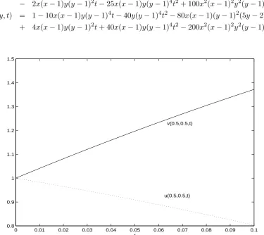
Figure 1. Two term - decomposition series solutions (u, v) with Du = 1
0 0.05 0.1 0.15 0.2 0.25 0.3 0.35 0.4 0.45 0.5 0.7
0.8 0.9 1 1.1 1.2 1.3 1.4 1.5
t
u(0.5,0.5,t) v(0.5,0.5,t)
Figure 2. Numerical solution of (4)-(6) with Du = Dv = 0 showing the
densities of di- vacancies (u) and vacancies (v).
0 0.05 0.1 0.15 0.2 0.25 0.3 0.35 0.4 0.45 0.5 0.8
0.85 0.9 0.95 1 1.05 1.1 1.15
t
u(0.5,0.5,t) v(0.5,0.5,t)
Figure 3. Numerical solution of (4)-(6) withDu = 1 andDv = 4 showing
4. Conclusion and results
In this paper, we have solved numerically a two dimensional diffusion reaction problem modelling the density of di-vacancies and vacancies in a metal. To do this, in the first we have used a decomposition method to get the series solution of the model. Further, we have obtained the numerical solution by the method of lines (MOL). MOL is a technique for solving partial differential equations in which all but one dimension is discretized. MOL most often refers to the construction or analysis of numerical methods for partial differential equations that proceeds by first discretizing the spatial derivatives only and leaving the time variable continuous. This leads to a system of ordinary differential equa-tions to which a numerical method for initial value ordinary equaequa-tions can be applied. In [8,16] the initial boundary value problem (4)-(6) has been solved by explicit and implicit methods, and stability and convergence of the problem were discussed there. However, we know that the explicit method is conditionally stable and the implicit method is time consuming.
Figure 1 shows the two-term series solution of the model obtained by Adomians polyno-mial whereas Figure 3 shows the numerical solutions obtained by MOL. We have achieved a very good approximation to the numerical solutions until approximatelyt= 0.05, which shows that the speed of convergence of decomposition method is very fast [4]. Also, one gets a very close approximation untilt= 0.5 by adding new terms to the series (24), which is tedious, so that the overall errors can be made pretty small. Therefore, the constantT0 must be chosen small for convergence purposes.
In Figure 2, we present the numerical solutions of the model with zero diffusions to see the behaviour of the densities of di-vacancies and vacancies compared to the nonzero diffusions case (drawn in Figure 3). Apparently these two figures look similar untilt= 0.05. After that time, the solutions tend to constant solutions in the nonzero diffusions case while the solutions separate in the zero diffusions case.
In conclusion, Adomians decomposition method provides very accurate numerical solu-tions for nonlinear problems in comparison with other methods [4]. It also does not require large computer memory and discretization of the variables and avoids linearization and physically unrealistic assumptions.
Acknowledgement
The author thanks to Assoc. Prof. Dr. Umit Kadiroglu of the department of chemistry of Kocaeli University/Turkey for suggesting me some nice references related to diffusion of di-vacancies and vacancies in a metal.
References
[1] Adomian,G., (1994), Solving Frontier Problems of Physics: the Decomposition Method, Kluwer Academic Publishers, Boston.
[2] Ali,E.J., (2012), A New Technique of Initial Boundary Value Problems Using Adomian Decompo-sition Method, Int. Math. Forum., 7 (17), pp. 799–814.
[3] Brandes,E.A. and Brook,G.B., (1992), Smithells Metals Reference Book, Seventh Edition, Butterworth-Heinemann, Oxford.
[4] Cherruault,Y. and Adomian,G., (1993), Decomposition methods: a new proof of convergence, Math. Comp. Model., 18, pp.103-106.
[5] Dieter,G.E., (1986), Mechanical Metallurgy, Third Edition, McGraw-Hill, New York.
[6] Dudarev,S.L., (2013), Density Functional Theory Models for Radiation Damage , Annu. Rev. Mater. Res., 43, pp.35-61.
[8] Hoang,S., Baraille,R., Talagrand,O., Nguyen,T.L., and De Mey,P., (1997), Approximation approach for nonlinear filtering problem with time dependent noises, Kybernetika., 33(5), pp.557-576.
[9] Kailas,S.V., Material Science: Diffusion.pdf. Retrieved from http://www.nptel.ac.in/courses/ 112108150/pdf/LectureNotes/MLN05.pdf
[10] Kaya,D. and Yokus,A., (2002), A numerical comparison of partial solutions in the decomposition method for linear and nonlinear partial differential equations, Math. Comput. Simulat., 60, pp.507-512.
[11] Kaya,D. and Aassila,M., (2002), An application for a generalized KdV equation by the decompo-sition method, Phys.Lett. A., 299, pp.201-206.
[12] Malik,R., Burch,D., Bazant,M., and Ceder,G. , Particle Size Dependence of the Ionic Diffusivity, DOI: 10.1021/nl1023595, Retrieved from pubs.acs.org/NanoLett.
[13] Pamuk,S. , (2005), The decomposition method for continuous population models for single and interacting species, Applied Mathematics and Computation., 163(1), pp.79-88.
[14] Pamuk,S., (2005), An application for linear and nonlinear heat equations by Adomians decompo-sition method, Applied Mathematics and Computation, 163(1), pp.89-96.
[15] Pamuk,S., (2005), Solution of the porous media equation by Adomians decomposition method, Physics Letters A., 344 (2-4), pp.184-188.
[16] Sewell,G., (1988), The numerical Solution of Ordinary and Partial Differential Equations. Aca-demic Press, New York.
[17] Shewmon,P.G., (1989), Diffusion in Solids, Second Edition, The Minerals, Metals and Materials Society, Warrendale, PA.
[18] Sterne,P.A., J. van Ek, and Howell,R.H., (1997), Electronic Structure Calculations of Vacancies and Their Influence on Materials Properties, UCRL-JC-127349, Preprint.