Engineering Volume 2, 2018, Pages 173–182
SUMO 2018- Simulating Autonomous and Intermodal Transport Systems
Route estimation based on network flow maximization
Michael Behrisch and Jakob Erdmann
Institute of Transportation Systems, German Aerospace Center, Berlin, Germany
Abstract
We present an algorithm which calculates a list of routes in a street network, approxi-mating the flows given on the streets by traffic counts. We prove optimality with respect to maximizing the flows treating the counts as constraints and show that the algorithm can cope very well with missing data using a real motorway example.
1
Introduction
One of the main problems occurring (not only) in the context of doing a microsimulation of real traffic networks which should resemble real data is traffic (or route) assignment. That is, give each car a route such that the real traffic situation is well reflected. There may be several sources of input to this problem, such as origin destination matrices, junction turn ratios, and traffic counts on individual streets and all of them may come with a different time resolution. Furthermore it is a highly dynamic problem because small changes in the traffic situation may induce completely different route choices for a lot of drivers.
The part of the problem we will solve in this article is the static subpart, if we are given traffic counts for the streets of a network. The objective is to find a list of routes such that the total number of cars driving on each street approximates the measured traffic counts best possible. The dynamics of the driving behavior is not taken into account, thus starting times and velocities do not matter, the only objective is to approximate the number of cars using each single edge in a best possible manner.
We will view the street network as a directed graphG= (V, E) with vertex (junction) set
V and edge (street) setE ⊆ V ×V, together with a set of source vertices S ⊆V and a set of target verticesT ⊆V withS∩T =∅. Let Γ+(v) denote for each vertex v ∈V the set of vertices which can reached fromv by following edges (successors) and Γ−(v) the set of vertices from whichv can be reached (predecessors).
The traffic counts are given by a function c : E → N, where N are the natural numbers
starting with 0 and including an infinite value, denoted by ∞ which stands for a number larger than any number occurring in the calculations performed withc(probably 1 +P
e∈Ec(e)
suffices).
which visit vertices and even edges twice. LetR(G) denote the set of all possible routes in the graphG, then the solution presented by the algorithm is a list d= (r1, . . . , rk) of routes with
r1, . . . , rk ∈R(G).
Let #(a, L) denote the element count function, which gives for a list of elements L = (a1, . . . , an) with a1, . . . , ak ∈A and an element a∈ A the number of occurrences of a in L, Given the route list D it is possible to calculate for each edge a load wd : E → N which is
defined as
wd(e) :=
X
r∈R
#(r, d)·#(e, r). (1)
In a slight abuse of notation and to save parentheses, we will writef(a, b) instead off((a, b)) whenever we talk about a function value of an edge pointing fromatob. Furthermore we write
h:=f −gto abbreviateh(e) :=f(e)−g(e) for alle∈E.
We will show that we can find a route list d such that the resulting loadw approximates the traffic counts well from below, precisely we will minimize
X
e∈E
c(e)−wd(e) (2)
under the condition thatwd(e)< c(e) for all edges e.
The objective function (2) has an equivalent formulation as maximizing
X
e∈E
wd(e) (3)
with respect towd(e)< c(e) for all edgese. The problem is solved in two steps.
1. Find a weight function which respects flow conservation (Kirchhoff’s law) and approxi-mates the traffic counts best.
2. Construct routes fitting the weight function.
where Kirchhoff’s law refers to the fact that for every vertex which is neither a source nor a sink, the sum of the incoming flow has to be equal to the sum of the outgoing flow.
The rest of the paper is organized as follows. After giving a short overview on related results in the rest of this section, the algorithm will be presented together with a precise statement of the results. Section3 will show, why it is possible to split the problem as stated and how to construct the routes from the weights. Afterwards (Section 4) it will be shown how to find the optimal load functionw(without knowing the route distribution) using network flow maximization techniques. We will then present the applications and extensions of the algorithm to a real motorway network. At the end there will be closing remarks on missing data and an outlook on the extensibility of the results.
1.1
Related work
The topic of route finding (or traffic assignment) has received considerable interest throughout the years. A good overview over the historical development as well as recent research concerning static and dynamic route assignment, can be found in [11,2].
In most algorithms the focus is on solving the dynamic problem either via mathematical programming, stochastical assignment (for instance using the path flow estimator [3]) or via
simulation [8]. From the static point of view there are almost always edge costs involved (see of [2, Chapter 5]) which give another piece of complexity, but the smaller problem discussed here seems to be almost unstudied. The usage of link flows to adjust routes with different algorithms has also been studied in [12].
For a good overview of the topic of network flows which are used to find the optimal route assignment the reader is referred to [1].
2
The algorithm
The main statement of this paper is as follows:
Given a directed graph G=(V,E) together with source and sink verticesS⊆V and
T ⊆V and a functionc:E→N, the algorithm FlowMax finds a route listdsuch that
X
e∈E
c(e)−wd(e)
is minimized with respect towd(e)< c(e) for all edges e∈E.
A short sketch of the algorithm looks as follows
Input: GraphG = (V, E), source set S, target set T, traffic count function
c:E→N
Output: route distributiond:R→N
FlowMax(G, S, T, c) (1) V :=V ∪ {s, t}; (2) foreachx∈S
(3) E:=E∪(s, x); (4) c(s, x) :=∞
(5) foreachx∈T
(6) E:=E∪(x, t); (7) c(x, t) :=∞
(8) w:=MaxNetworkFlow(G, s, t, c) (9) c:=c−w
(10) Mergesandtto a
(11) foreachv∈V
(12) Split the vertexvinvsandvtsuch that Γ−(vs) =∅and Γ+(vt) =∅
(13) w:=w+PositiveNetworkFlow(G, vs, vt, c)
(14) c:=c−w
(15) Mergevsandvt
(16) ConstructG0 by replacing every edgeebyw(e) unweighted edges (17) Find a Euler TourU = (e1, ..., ek) inG0
(18) d:=SplitU at all edges containinga
with a running time of less than C|V||E|2 [5]. We need a minor modification of this algo-rithm which only accepts flow increasing steps which increase the total flow in the network (PositiveNetworkFlow).
The second part of the algorithm, starting at line16will be described in more detail in the next section. The motivation for the network flow part is delayed to Section4.
3
Routes and flow conservation
It is easy to see, that for every route distributiondthe relevant weight functionwd, defined in
(1), satisfies Kirchhoff’s law for every non source or target vertex, thus if we define:
∆(u) = X
x∈Γ−(u)
w(x, u)− X
x∈Γ+(u)
w(u, x). (4)
we have
∆(u) = 0 foru∈V \(S∪T). (5)
Furthermore, we have that the amount of flow inserted at the sources is equal to the amount of flow leaving at the targets:
X
s∈S
∆(s) +X
t∈T
∆(t) = 0. (6)
Now it will be shown that in turn from every weight functionw which obeys (5) and (6) a route distributionscan be derived such that wd =w. If this is proven, the task of finding an
optimal route distribution is simplified to finding the optimal weight assignment with respect to the constraints, which is the topic of Section4.
3.1
Constructing routes from weights
Assume there is a weight function given which respects (5) and (6) If we introduce an auxiliary vertexawhich is connected to all sinks and all sourcesx∈S∪T using edges of weight ∆(x), we have a network respecting (5) in all vertices.
In order to construct the routes, we transform the weighted input graph (with the auxiliary vertex) into a directed unweighted multigraph by replacing every edge (u, v) of weight b =
w(u, v) withb edges connecting uand v. This graph has an Euler tour (a cycle which visits each edge exactly once), which can be found in linear time by repeated depth first search [4].
Having a directed tour which visits each edge once, it is possible to remove the auxiliary vertex again and end up with a number of routes which exactly resemble the weights. Note that this procedure only works because we allow for routes which contain the same edge multiple times.
4
Flow maximization
This section will show how to assign weights to the edges of the input graph such that the total weight is maximized, while w(e) < c(e) for everye ∈E(G). We will do so by describing the way the FlowMax algorithm works. The first part of the algorithm just resembles a standard technique to simplify the problem to a single source and a single sink. After having performed the first flow maximization step in line 8 the flow through the network is maximal, which means, it is not possible to increase the total number of cars driving through the network.
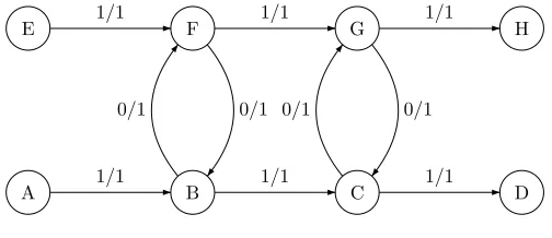
While this result respects both (5) and (6) and maximizes the flow on at least one edge, it may not maximize the flow on each individual edge, as is shown in Figure 1 where the edges are labeled with ”weight / capacity”, the sources are A and E and the sinks D and H.M. Behrisch 5
A B C D
E F G H
1/1 1/1 1/1
1/1 1/1 1/1
0/1 0/1 0/1 0/1
Figure 1A maximum net flow which does not maximize all edge flows
G. Those two cycles are obviously found in our post optimization step, which gives full saturation to all edges.
Assume now that the algorithm is in a stage where there are still edges which do not have maximal flow and the present weight assignment isw. Furthermore let ˆwdenote the weight assignment of a maximizing solution.
4.1 Missing data
It is possible to let the algorithm run without a complete set of traffic count data. If we assign∞to all edges where data is missing it will still approximate the rest of the edges
best possible as long as there is no source-sink-path and no directed cycle in the graph consisting only of edges without data. Even in this case the algorithm may still work with minor modifications to the flow maximization steps, but it is harder to proof optimality in this case.
5 Summary and Outlook
We presented an algorithm which calculates solely on the basis of traffic count data a list of routes optimally resembling this data. It employs network flow maximization as a black box which allows for the usage of highly optimized flow algorithms in the implementation of the algorithm. Furthermore it can handle the case of missing data very well, it does not even need a complete set of information for the edges surrounding sinks or sources. Finally the separation of the approximation of the traffic counts and the actual route finding allows for the optimization (or even replacement) of one of the strategies without affecting the other part, for instance to meet different objectives as discussed below.
The algorithm is already implemented as a prototype inside the simulation software package SUMO [8, 7]. The first results concerning quality and runtime are very promising, but there are not enough results on real yet, thus the practical evaluation will follow in another article. Two additional topics may be of interest for further studies, which will be discussed in the following subsections.
5.1 Self disjoint routes
Although it is a perfectly valid assumption regarding Kirchhoff’s law and is probably even found in the real world, it is often not desirable to have routes which visit vertices or even edges twice. This requirement leads to a problem, which cannot be solved optimally with
Figure 1: A maximum net flow which does not maximize all edge flows
For a motivation, why the algorithm works, please note that in the network given in Figure 1the non saturated edges come in two cycles joining B and F, respectively C and G. Those two cycles are found in our post optimization step, which gives full saturation to all edges.
4.1
Missing data
It is possible to let the algorithm run without a complete set of traffic count data. If we assign
∞to all edges where data is missing it will still approximate the rest of the edges best possible as long as there is no source-sink-path and no directed cycle in the graph consisting only of edges without data. Even in the latter case the algorithm still works with minor modifications to the flow maximization steps, which abort the search when an infinte cycle or path has been found but it is not possible to proof optimality in this case because a maximum does not exist. The feature of reconstructing missing values basically by the means of the flow conservation equation is the main feature why the algorithm should perform better than the existing dfrouter algorithm.
4.2
Tweaking the algorithm for more realistic routes
Since the algorithm to find the routes is basically looking for cycles in a multi-graph, it has the risk of finding very short routes because it employs a depth first search strategy. Furthermore it may put too much emphasis on first satisfying a single detector value before it is looking for other options simply because it comes first in its list. To overcome this limitations in the implementation of the algorithm the two steps of finding the maximum flow and determining the routes have been integrated which gives the possility to direct the route finding into edges where still much flow is missing or where the solution seems unbalanced because maybe an off-ramp attracts much more flow than the main track.
Two further points are to add articial limitations stemming from the number of lanes of an edge to direct the algorithm to realistic solutions or limiting the search to start only on edges which have measured data to avoid high inflows at unrealistic positions. Both aproaches can be used as some kind of preprocessing to start with a good solution which is still tobe optimized by the unlimited search but gives more realistic routes.
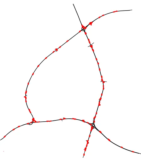
Figure 2: Street Network with induction loops in the Real-World A9 Scenario
These tweaks should not affect the general optimality result but only give better results concerning the length and overall structure of the routes. To give even more control, the implementation also allows to forbid certain routes explicitly for instance because they contain unwanted loops.
To direct the algorithm to good solutions it is useful to apply different values for the capacity functioncin the first flow maximization step and in the second edge weight maximization step. The reason to do this is that the maximization of the edge flow should only consider edges which have real detector data available and are not artificially limitted by the means described above.
5
Real world example
The algorithm has been applied to a highway network in the north of Munich which consists of three major arteria A9, A92 and A99 connected at three crosses and several on and off-ramps (see Figure2).
It is covered by 282 induction loop detectors at 118 cross sections which give data for almost every part of the network. The detector set has been cleaned manually with removing all cross sections where not all lanes of the motorway were covered or had large deviations between the lanes. Furthermore for each part of the motorway berween consecutive ramps only the cross section with the maximum measured flow was used.
The detector data used one full day of collected traffic counts from the 20th of May2014.
It has been restricted to passenger cars and split into two data sets one for the whole day and one for the morning peak hour from 7 to 8. It was always aggregated over the whole period. The algorithm is sensitive and for the whole cross section (so no lane assignment was done).
5.1
Evaluation
Since there is no data available to us on the real world route choice, the results are only compared how good they approximate the measured flow data. The problem with the comparison are the different scales of the input data where low volume ramps are up to a factor of 10 away from the high volume main tracks. So it is necessary to find a measurement which gives neither too much weight to relative errors because that favors the main track nor to absolute erros which would favor the ramps. One such measurement is the so-called GEH [6] (named after Geoffrey E. Havers) value which is calculated as
GEH(e) =
s
2(w(e)−m(e))2
w(e) +m(e) (7)
wherem(e) denotes the measurement on edgeeandw(e) the assigned weight by the algorithm. When applied to hourly measurements a GEH of smaller than 10 is usually an accepatable value while a GEH smaller than 5 is a good result.
The major feature of the presented algorithm is presumably its ability to cope with missing data. In order to validate this assumption and at the same time to give results which can be transferrable from a network being heavily covered with detector to less well equipped areas, the following setup has been chosen. Instead of calculating the routes based on all detectors, a fixed percentage of the detectors was removed before doing the calculation. Using this method a variation could be introduced as well, allowing to create multiple different data points from the same scenario by choosing different detectors to remove uniformly at random.
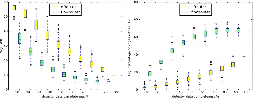
All experiments were performed iwth the same input data but a variation was only possible when detectors were removed, so the 100% sample has no variation. The following plots present box plots (showing the median and the first and the third quartile in the box) of the average GEH value on all edges which have measurements (not only on the selected detectors). The variation comes from 100 route calculation runs where different detectors (but always the given percentage) were used for calculating the routes. The comparison is always done between the dfrouter values (yellow, on the left) and the flowrouter algorithm (green, on the right).
The first experiments shown in Figure3gave mixed results where the flowrouter could only excel with very few given data points (although the resulting GEH is here already much above the point of a good fit) and with complete data. While it was at first assumed that this is due to dynamic effects (vehicles taking time to travel through the network which is not fully reflected when the data covers only an hour) the results for the full day (second plot) show the same pattern although they show smaller GEH values in general.
Figure 3: GEH values when removing random detectors in the peak hour (left) and the full day (right)
Figure 4: GEH values when removing random cross sections in the peak hour
The second plot in Figure4shows that the flowrouter is not only able to have a much smaller average GEH but also performs better on the edges which are considered to be approximated well (GEH smaller than 5).While the dfrouter can only fit less than 40% even with full data inputs, the flowrouter reaches this quality already with 40% of the input data. Our data also shows that the flowroute indeed sometimes benefits from the removal of some detectors such that it can calculate a better total approximation in terms of the GEH. While this needs further research it likely stems again from the fact that the flowrouter always takes the measurements as a maximum while the GEH allows deviations in both directions.
Our experiments show clearly that while the flowrouter can cope better with mssing data it can also get easily confused with only partially correct data (e.g. with single lane data missing fom a cross section). The good news here is that it is usually not too hard to detect such cases.
6
Summary and Outlook
We presented an algorithm which calculates solely on the basis of traffic count data a list of routes optimally resembling this data. It employs network flow maximization as a black box which allows for the usage of highly optimized flow algorithms in the implementation of the algorithm. Furthermore it can handle the case of missing data very well, it does not even need a complete set of information for the edges surrounding sinks or sources. Finally the separation of the approximation of the traffic counts and the actual route finding allows for the optimization (or even replacement) of one of the strategies without affecting the other part, for instance to meet different objectives as discussed below.
The algorithm is already implemented as a prototype inside the simulation software package SUMO [10,9]. The first results concerning quality and runtime are very promising, but thereis need for more evaluation especially in the case of single detector being missing at across section. Two additional topics may be of interest for further studies, which will be discussed in the following subsections.
6.1
Alternative objective functions
Our objective function looks quite unusual, because normally one tries to minimize something like the sum of the squared distances of the values. One way to let at least the mean flows match is to execute the algorithm repeatedly, increasing the capacity of all saturated edges by the difference of the mean traffic count and the mean flow calculated. Furthermore the algorithm woukld benefit from apriori knowledge about the expected distribution of route lengths to generate more realistic routes.
6.2
Comparison with existing tools
There are several calibration and flow estimation tools available such as the Cadyts tool ([7]) or the Path flow estimator [3]. A future project would be to compre them to the presented algorithm especially with a focus on missing data but also to extend the topic to lane precise assignment or taking delays in the traffic flow into account.
References
[1] R. K. Ahuja, T. L. Magnanti, and J. B. Orlin.Network flows: theory, algorithms and applications. Prentice-Hall, Englewood Cliffs NJ, 1993.
[2] M. O. Ball, T. L. Magnanti, C. L. Monma, and G. L. Nemhauser, editors. Network Routing. Handbooks in OR & MS, Vol. 8. Elsevier, Amsterdam, 1995.
[3] M. G. H. Bell, C. M. Shield, F. Busch, and G. Kruse. A stochastic user equilibrium path flow estimator. Transportation Research Part C: Emerging Technologies, 5(3):197–210, 1997.
[4] T. H. Cormen, C. E. Leiserson, R. L. Rivest, and C. Stein. Introduction to algorithms. The MIT Press, 2 edition, 2001.
[5] J. Edmonds and R. M. Karp. Theoretical improvements in algorithmic efficiency for network flow problems. Journal of the Association for Computing Machinery, 19(2):248–264, 1972.
[6] O. Feldman. The GEH measure and quality of the highway assignment models. Association for European Transport and Contributors, pages 1–18, 2012.
[7] G. Fl¨otter¨od, M. Bierlaire, and K. Nagel. Bayesian demand calibration for dynamic traffic simu-lations. Transportation Science, 45(4):541–561, 2011.
[9] D. Krajzewicz. SUMO homepage. http://sumo.sourceforge.net/, accessed August 1, 2007. [10] D. Krajzewicz, M. Hartinger, G. Hertkorn, E. Nicolay, C. R¨ossel, J. Ringel, and P. Wagner.
Recent extensions to the open source traffic simulation SUMO. InProceedings of the 10th World Conference on Transport Research (on CD), 2004.
[11] M. Patrikson, editor. The Traffic Assignment Problem – Models and Methods. Topics in Trans-portation. VSP, Utrecht, The Netherlands, 1994.
[12] T. Tsekeris and A. Stathopoulos. Real-time dynamic origin-destination matrix adjustment with simulated and actual link flows in urban networks. InTransportation Research Record 1857, pages 117–127, Washington, D.C., 2003. TRB, National Research Council.