https://doi.org/10.5194/gmd-12-3585-2019 © Author(s) 2019. This work is distributed under the Creative Commons Attribution 4.0 License.
Global simulation of semivolatile organic compounds – development
and evaluation of the MESSy submodel SVOC (v1.0)
Mega Octaviani1, Holger Tost2, and Gerhard Lammel1,3
1Multiphase Chemistry Department, Max Planck Institute for Chemistry, 55128 Mainz, Germany 2Institute for Atmospheric Physics, Johannes Gutenberg University of Mainz, 55099 Mainz, Germany
3Research Centre for Toxic Compounds in the Environment, Masaryk University, 62500 Brno, Czech Republic
Correspondence:Gerhard Lammel ([email protected])
Received: 21 January 2019 – Discussion started: 28 February 2019
Revised: 18 June 2019 – Accepted: 10 July 2019 – Published: 19 August 2019
Abstract. The new submodel SVOC for the Modular Earth Submodel System (MESSy) was developed and ap-plied within the ECHAM5/MESSy Atmospheric Chemistry (EMAC) model to simulate the atmospheric cycling and air–surface exchange processes of semivolatile organic pol-lutants. Our focus is on four polycyclic aromatic hydro-carbons (PAHs) of largely varying properties. Some new features in input and physics parameterizations of tracers were tested: emission seasonality, the size discretization of particulate-phase tracers, the application of poly-parameter linear free-energy relationships in gas–particle partitioning, and re-volatilization from land and sea surfaces. The results indicate that the predicted global distribution of the 3-ring PAH phenanthrene is sensitive to the seasonality of its emis-sions, followed by the effects of considering re-volatilization from surfaces. The predicted distributions of the 4-ring PAHs fluoranthene and pyrene and the 5-ring PAH benzo(a)pyrene are found to be sensitive to the combinations of factors with their synergistic effects being stronger than the direct effects of the individual factors. The model was validated against observations of PAH concentrations and aerosol particulate mass fraction. The annual mean concentrations are simulated to the right order of magnitude for most cases and the model well captures the species and regional variations. However, large underestimation is found over the ocean. It is found that the particulate mass fraction of the benzo(a)pyrene is well simulated, whereas those of other species are lower than ob-served.
1 Introduction
The atmospheric cycling of semivolatile organic compounds (SOCs) is particularly complex because of partitioning across phases and air–surface exchange processes, including multihopping (or “grasshopper effect”; Semeena and Lam-mel, 2005) and accumulation in ground compartments such as seawater, soil, vegetation, and ice/snow. Many SOCs do resist degradation in environmental compartments, and hence are persistent. In the regulation of chemical substances and in international chemicals legislation (e.g., UNEP, 2017), model-based quantifications of the overall environmental res-idence times (persistence) and the long-range transport po-tentials are requested or encouraged to be applied.
a chemistry module describes the changes in air concen-trations due to phase partitioning and chemical transforma-tions. Compared to the multimedia models, CTMs have bet-ter spatial and temporal resolutions but require more com-putational effort. They are suitable for use to investigate the variability and episodic character of environmental fate and transport. To date, pollutants addressed in model studies were persistent organic pollutants, such as dichlorodiphenyl-trichloroethane (DDT), polychlorinated biphenyls (PCBs), hexachlorocyclohexanes (HCHs), polycyclic aromatic hy-drocarbons (PAHs), and more recent so-called emerging pol-lutants (e.g., MacLeod et al., 2011).
The sensitivity of distributions to specific processes of SOC cycling and related input parameters has been the fo-cus of CTM-based studies (Semeena et al., 2006; Sehili and Lammel, 2007; Friedman and Selin, 2012; Galarneau et al., 2014; Thackray et al., 2015). Sehili and Lammel (2007), for instance, suggest that the gas–particle partitioning and particulate-phase oxidation scenarios have significant influ-ences on the long-range atmospheric transport of PAHs. This finding is supported by Friedman and Selin (2012), who fur-thermore concluded that the effects are higher than those of irreversible partitioning and of increased aerosol concentra-tions.
This study presents the new multicompartment module (submodel) SVOC for the Modular Earth Submodel Sys-tem (MESSy; Jöckel et al., 2006, 2010). MESSy provides a modular framework for simulations accounting for vari-ous degrees of complexity and to facilitate continuvari-ous fu-ture submodel improvements. The submodel has been ap-plied using the general circulation model ECHAM5 (Roeck-ner et al., 2003, 2006) as a base model. In connection with the ECHAM5/MESSy Atmospheric Chemistry (EMAC) model, SVOC encompasses a 3-D atmosphere and 2-D surface com-partments (soil, vegetation, snow, and ocean mixed layer), and considers multicompartment fate and exchange pro-cesses, such as emission, phase partitioning, wet and dry de-position of gases and particles, degradation, and air–surface gas exchange, including re-volatilization. SVOC is devel-oped and intended to be applied for the study of all po-tentially re-volatilizing and gas–particle-partitioning (hence semivolatile) compounds. Nevertheless, the focus of this sub-model development is the global distribution of four PAH species of largely varying properties. PAHs enter the atmo-spheric environment as by-products of all technological com-bustion processes (Shen et al., 2013) and of open fires (Gul-lett et al., 2008). They are ubiquitous pollutants of partic-ular environmental and health concern (WHO, 2003; Laen-der et al., 2011; Lammel, 2015) and due to their continu-ous global emissions. Here we describe the submodel devel-opment, compare the results to observations, and assess the significance of four model features to PAH distributions and fate. These features are the temporal resolution of emissions, the size discretization of particulate-phase tracers (bulk or
modal), the choice of the gas–particle partitioning scheme, and re-volatilization from surfaces.
2 Methods
2.1 Model descriptions
The global model applied in this study is the ECHAM5/MESSy Atmospheric Chemistry Climate model (EMAC), a three-dimensional Eulerian model for the simu-lations of meteorological variables, gases, aerosols, clouds, and other climate-related parameters. EMAC combines the general circulation model ECHAM5 (here version 5.3.02) (Roeckner et al., 2003, 2006) with the Modular Earth Submodel System (MESSy version 2.50; Jöckel et al., 2006, 2010). The atmospheric component of ECHAM5 derives four prognostic variables, namely vorticity, divergence, tem-perature, and the logarithm of surface pressure in truncated series of spherical harmonics, whereas specific humidity, cloud water, and cloud ice are represented in grid point space. MESSy provides a modular framework to define atmospheric dynamics, chemistry, transport, and radiative transfer processes. For a more detailed description of the EMAC model, evaluation and relevant studies, refer to Jöckel et al. (2006, 2010) and http://www.messy-interface.org (last access: 12 July 2019). The list of MESSy process-based modules, hereinafter submodels, applied in this study are summarized in Table 1.
The new MESSy submodel SVOC for simulating the fate and cycling of SOCs in the global environment is presented. Processes involved in the submodel include gas–particle par-titioning, volatilization from the surface, dry and wet de-positions, and chemical and biotic degradations. These pro-cesses are connected to other MESSy submodels. For exam-ple, deposition of gas-phase SOCs are calculated by the sub-models SCAV and DDEP, aerosol microphysics by GMXe, gas-phase chemistry mechanisms by MECCA, and ocean– air flux exchange by AIRSEA. Figure 1 illustrates the SVOC structure within the EMAC system and its interactions with other MESSy submodels. More details on some process pa-rameterizations are given in the following section. A user manual can be found in the Supplement with the list of sub-model input and output variables.
2.2 Parameterizations of cycling processes in multiple compartments
Table 1.Summary of MESSy process submodels used in this study.
Submodel Purpose Reference
AEROPT Aerosol optical properties Lauer et al. (2007)
AIRSEA Air–sea exchange Pozzer et al. (2006)
CLOUD ECHAM5 cloud and precipitation scheme as MESSy submodel Roeckner et al. (2006) and references therein CONVECT Convection parameterizations Tost et al. (2006b, 2010)
CVTRANS Convective tracer transport Tost (2006)
DDEP Dry deposition of gases and aerosols Kerkweg et al. (2006a) GMXe Aerosol dynamics and thermodynamics Pringle et al. (2010)
JVAL Rate of photolysis based on Landgraf and Crutzen (1998)
LNOX NOxproduction from lightning Tost et al. (2007)
MECCA Tropospheric and stratospheric chemistry Sander et al. (2011)
OFFEMIS Offline emissions Kerkweg et al. (2006b)
ONEMIS Online emissions Kerkweg et al. (2006b)
RAD ECHAM5 radiation scheme as MESSy submodel Roeckner et al. (2006); Jöckel et al. (2006) SCAV Scavenging of gases and aerosols Tost et al. (2006a)
SEDI Aerosol sedimentation Kerkweg et al. (2006a)
Figure 1.Overview of EMAC-SVOC model structure, the cycling processes in SVOC submodel, and its interaction with other MESSy submodels. SMIL (submodel interface layer) and SMCL (submodel core layer) are components of MESSy coding standard, see Jöckel et al. (2006) for further details.
sizes are resolved into n continuous (modal) distributions. The former will be hereinafter referred to as thebulkscheme and the latter referred to as themodalscheme. In the modal scheme, n is equal to the seven log-normal modes of the GMXe submodel, four with hydrophilic coating (ns: nucle-ation soluble, ks: Aitken soluble, as: accumulnucle-ation soluble, cs: coarse soluble) and three hydrophobic (ki: Aitken insolu-ble, ai: accumulation insoluinsolu-ble, ci: coarse insoluble) (Pringle et al., 2010). Each mode is treated as an individual tracer.
2.2.2 Partitioning between gas phase and particulate phase
Gas–particle partitioning is assumed to take place when SOC is in equilibrium between the gas and particulate phases. The concentration of the species that is bound to particles (Cparticle) is calculated with
and the particulate mass fraction (θ) is defined as
θ= Cparticle Cparticle+Cgas
= Kp×CPM 1+Kp×CPM
= K
0
p
1+K0
p
, (2)
whereCPMis the concentration of particulate matter or PM
(µg m−3),Kpis the temperature-dependent particle–air
par-tition coefficient (m3µg−1), andKp0 is the dimensionlessKp.
In a model configuration using size-resolved particles (viz. the modal scheme), each SOC tracer is introduced in the model as eight different species: seven aerosol particles in ns, ks, as, cs, ki, ai, ci modes and one in the gas phase. The par-ticulate fraction of the species in modei(θi) is calculated us-ing Eq. (2) withCPMiandKpi being the PM mass
concentra-tion and aerosol–air particoncentra-tion coefficient in the corresponding mode, respectively. The gaseous concentrationCgasis
calcu-lated using the sum of Kp values across modes, as well as
totalCparticleandCPM:
Cgas= 7 P i=1
Cparticlei/ 7 P i=1
CPMi
7 P i=1
Kpi
. (3)
It is noted that this approach may not hold the constraint of mass consistency and is thus subject to further corrections. For the current study, the effects from this problem are ex-pected to be minimal, given the fact that PAHs in the partic-ulate phase are mainly distributed in the accumulation mode (Lammel et al., 2010, and references therein).
ForKp calculation four options of gas–particle
partition-ing schemes are available in SVOC: (1) a parameterization that is based on adsorption onto aerosol surface (Junge, 1977; Pankow, 1987), (2) absorption into organic matter (Finizio et al., 1997), (3) a combination of the two ways of organic matter absorption and black carbon adsorption (Lohmann and Lammel, 2004), and (4) multiple phases of the two-way sorption system (Goss and Schwarzenbach, 2001; Endo and Goss, 2014; Shahpoury et al., 2016). Two schemes used in this study are described below.
– Lohmann–Lammel scheme. The Lohmann–Lammel scheme takes into account an adsorption onto black car-bon (BC) surface in addition to absorption into organic matter (OM) (Lohmann and Lammel, 2004). This dual-sorption theory empirically calculates Kp according to
the following relation, Kp=10−12
fOM
γoctMWoct γOM MWOM ρoct
Koa
+fBC
aatm-BC asoot ρBC
Ksa
, (4)
whereρBCis the density of BC (assumed as 1 kg L−1), ρoct is the density of octanol (0.82 kg L−1 at 20◦C),
Ksa is the partition coefficient between diesel soot and
air,aatm-BCis the available surface of atmospheric BC
(m2g−1), anda
sootis the specific surface area of diesel
soot (m2g−1). The adsorptive properties of diesel soot are selected to represent the atmospheric BC because this material is considered the most significant type of BC in polluted air.
TheKsavalue is calculated as a function of sub-cooled
liquid vapor pressurep0Lusing an estimate suggested by van Noort (2003),
logKsa= −0.85 logpL0+8.94−log 998
asoot
, (5)
whereasootin the model is set as 18.21 m2g−1.
– Poly-parameter linear free-energy relationships (ppLFER) scheme. The concept of poly-parameter linear free-energy relationships (ppLFER) for the prediction of equilibrium partition coefficients is introduced by Goss and Schwarzenbach (2001), and its application in environmental chemistry has been reviewed by Endo and Goss (2014). This approach can describe a composite of different types of interactions between gas-phase species and aerosols. In contrast, single-parameter LFERs only correlate the partition coefficient to the sub-cooled liquid vapor pressure or the octanol–air partition coefficient of the species, and hence only valid within the group of compounds for which they were developed.
In the study, the ppLFER scheme is incorporated into SVOC in which it defines Kp as the sum of
individ-ual partition coefficients representing surface adsorp-tion and bulk-phase absorpadsorp-tion processes to inorganic and organic aerosols. The formulation ofKpis adopted
from Shahpoury et al. (2016) and is described as follows
Kp=
Kp0
CPM
,
Kp0=KEC×aEC×CEC×10−6 +
K(NH4)2SO4×a(NH4)2SO4×C(NH4)2SO4×10
−6+
KNaCl×aNaCl×CNaCl×10−6 +
KDMSO×
CWSOM
ρDMSO
×10−6 +
KPU×0.2×CWIOM×10−12 +
Khexadecane×0.8×
CWIOM
ρhexadecane
×10−6, (6)
where KEC, K(NH4)2SO4, and KNaCl are the
(absorption) coefficient for the dimethyl sulfoxide– air system (LairL−DMSO1 ). KPU is the substance
par-tition (absorption) coefficient for the polyurethane– air system (m3airkg−PU1). Khexadecane is the substance
partition (absorption) coefficient for the hexadecane– air system (LairL−hexadecane1 ); aEC, a(NH4)2SO4, and
aNaCl are the adsorbent-specific surface areas: 18.21,
0.1, and 0.1 m2surfaceg−adsorbent1 , respectively.ρDMSOand ρhexadecane are the dimethyl sulfoxide and hexadecane
densities of 1.1×10⁶ and 0.77×10⁶g m−3, respec-tively. CEC, C(NH4)2SO4, CNaCl, CWSOM, CWIOM are
the concentration (µgsubstancem−air3) of elemental carbon
(here black carbon), ammonium sulfate, sodium chlo-ride, water-soluble organic matter, and water-insoluble organic matter, respectively.
The ppLFER scheme calculates the sorptive partition coefficient for every aerosol system, as summarized in Table S1 in the Supplement. Each coefficient requires information on system parameters (e,s,a,b,v,l), and the constantc, as shown in Table S2. The Abraham so-lute descriptors (E,S,A,B,V, andL) are substance specific; for the species selected in this study, refer to Table S6. All the predicted partition constants are ad-justed to environmental temperature using the van ’t Hoff equation
lnK(T )=lnK(T0)−
1H R
1 T −
1 T0
, (7)
where1H is the enthalpy of solvent–air phase trans-fer in joules per mole (J mol−1). This variable is system specific and calculated by applying the ppLFER equa-tions given in Table S3 and input parameters given in Table S4. The sequence ofKpcalculation from ppLFER
analysis in SVOC is illustrated in Fig. S1 in the Supple-ment.
2.2.3 Volatilization 1. Soil
For soil volatilization, two parameterization schemes are implemented in the SVOC submodel: the Jury scheme (Jury et al., 1983, 1990) and the Smit scheme (Smit et al., 1997). The latter was applied in the study which is based on the volatilization of pesticides from the surface of fallow soils (Smit et al., 1997). The volatilization occurs upon partitioning over three soil phases (solid, gas, and liquid). The concentration of the chemical in the soil system (kg m−3) is formulated as
Csoil=Q×Cvapor, (8)
and the capacity factorQis given by
Q=ψ+ϕKwa+ρsoilKwaKsl, (9)
whereψandϕare the volume fractions of air and mois-ture, respectively;ρsoil is the soil density; Kwa is the
water–air partition coefficient whereKwa=1/Kaw; and Kslis the solid–liquid partition coefficient.Kawis
cal-culated based on the Henry’s law constant:
Kaw=1/ (H RT ) and (10)
H=kH×exp −
1Hsoln
R 1
T − 1 T0
, (11)
where H is the temperature-adjusted Henry coef-ficient (M atm−1), R is the dry air gas constant (8.314 J mol−1K−1),T is the environment temperature (K),1Hsolnis the enthalpy of dissolution (J mol−1). Ksl can be set equal to the sorption coefficient to soil
organic matterKomtimes the fraction of organic carbon
in soilfOMs. SinceKomdata are not available, the
coef-ficient for sorption to soil organic carbonKocwas used
to estimateKsl:
Ksl=0.56KocfOMs . (12)
Mackay and Boethling (2000) has suggested a rea-sonably good regression relationship betweenKoc and
octanol–water partition coefficientKowfor PAHs:
log(Koc/1000)=0.823 log(Kow/1000)−0.727 . (13)
where the factor of 1000 is needed becauseKocandKow
are expressed in cubic meter per kilogram (m3kg−1), whereas in the original regression they used milliliter per gram (mL g−1).
OnceQis computed, the dimensionless fraction of the chemical in the gas phaseFgasis then calculated as
Fgas= ψ
Q . (14)
In the Smit scheme, an empirical relation was estab-lished betweenFgas and cumulative volatilization (CV
in percent of substance deposit). CV was determined based on field and greenhouse experiments with numer-ous pesticides at 21 d after application. For normal to moist field conditions, CV is expressed as
CV=71.9+11.6 log(100Fgas);
6.33×10⁻⁹< Fgas≤1, (15)
and for dry field conditions CV=42.3+9.0 log(100Fgas);
2. Vegetation
Smit et al. (1998) derived an equation for the cumula-tive volatilization, CV, from plants against vapor pres-surePv(mPa) at 7 d after application based on field and
climate chamber experiments of pesticide volatilization (Eq. 17).
CV=101.528+0.466 logPv;P
v≤10.3. (17)
For compounds withPvabove 10.3 mPa, CV is set at
100 % of deposit. Temperature adjustments were made forPvusing the Clausius–Clapeyron equation:
d(lnPv)
dT = − 1Hvap
RT2 . (18)
3. Snow and glaciers
The parameterization of substance loss by volatiliza-tion from snow pack follows Wania (1997), whereby the process is calculated using a consecutive cycle of an equilibrium partitioning among four phases followed by a contaminant loss. The four phases considered are liquid water, organic matter contained in the snowpack, snow pores (air), and an ice–air interface. Fugacity ca-pacity factors for these phases are expressed with the following relations:
air(mol m−3Pa−1), Za=1/RT ; (19a)
water(mol m−3Pa−1) ,
Zl= Kwa/RT =Kwa Za ; (19b)
organic carbon(mol m−3Pa−1) ,
Zo= Zl 0.41Kow0 ; (19c)
ice–air interface(mol m−2Pa−1) ,
zi= Kia/RT =Kia Za; (19d)
where R is the dry air gas constant (8.312 J mol−1K−1), T is the air temperature (K),Kwa is the water–air
par-tition coefficient (unitless), Kow0 is the dimensionless octanol–water partition coefficient, and Kia is the ice
surface–air partition coefficient (m).Kiaat 20◦C is
es-timated usingKwaand water solubilityCws (mol m
−3),
logKia 20◦C= −0.769 logCsw−5.97+logKwa , (20)
and further extrapolated to other temperatures using en-thalpy of condensation of solid (1Hsublin J mol−1),
logKia(T )=logKia 20◦C +0.8781Hsubl
2.303 R 1
T − 1 293
. (21)
An equilibrium fugacityfsis thereby determined by fs=
Msp
Za va+Zl vl+zi Asnowρmw+Zovo
, (22)
where Msp is the amount of chemical contained in
snowpack (the model here applies snow burden of the chemical in kg m−2) and va, vl, and vo are the
vol-ume fractions of air, liquid water, and organic matter in snowpack (m3m−3), respectively. For this study,vaand vlvalues are set to 0.3 and 0.1, respectively, whereasvo
is zero assuming no polluted snow. Asnow is the
spe-cific snow surface area (m2g−1). In Daly and Wania (2004), a value of 0.1 m2g−1 for Asnow was used for
snow accumulation period and a linear decrease from 0.1 to 0.01 m2g−1 was used during the snowmelt pe-riod. In SVOC submodel, a value of 0.025 m2g−1 is adopted forAsnowto represent a fairly aged snowpack. ρmwis the density of snowmelt water and here is taken
as 7×10⁵g m−3.
Volatilization rate (kg m−2s−1) is calculated by apply-ing
dMsp
dt =
1
1
U7 Za+ 1
U5 Zl +U6 Za
×fs hs
, (23)
wherehs is the snow depth (m),U5is the snow–water
phase diffusion mass transfer coefficient (m h−1),U6is
the snow–air phase diffusion mass transfer coefficient (m h−1), andU7 is the snow–air boundary layer mass
transfer coefficient (m h−1).U5 andU6 are calculated
from molecular diffusivities in air and water (Eqs. 24 and 25), whereas a typical value of 5 m h−1is adopted forU7.
U5=Bw
vl10/3/(va+vl)2
ln 2hs
, (24)
U6=Ba
v10a /3/(va+vl)2
ln 2hs
, (25)
where Bw and Ba are the molecular diffusivities
(m2h−1) in water and air, respectively. In the model, Bais derived from the molecular weight (MW) asBa=
1.55 MW0.65cm
2s−1, whereasB
wis set as 1×10⁴less than Ba, following Schwarzenbach et al. (2005).
4. Ocean
et al., 2006). Note that no ocean and sea-ice dynamics were included in the simulations.
Sorption of SOCs in water to suspended particulate mat-ter (colloidal or sinking detritus) is neglected. There-fore, SOC concentration in surface seawater, and hence volatilization from sea surface, is overestimated, in par-ticular for very lipophilic (logiKow>6) substances.
This bias is negligible for the substances studied here (PAHs), which are less lipophilic or volatilization is lim-ited by vapor pressure (e.g., benzo(a)pyrene). Forces from strong winds and dissolved or particulate organics in seawater are transferred to air via sea spray, which adds to particulate OM in air over the ocean (O’Dowd et al., 2008; Qureshi et al., 2009). This process is ne-glected in the model.
2.2.4 Dry deposition
Dry deposition is simulated using deposition velocities. For gas-phase SOCs, the velocities are calculated by the DDEP submodel (Kerkweg et al., 2006a), whereas particulate-bound SOCs are assumed to deposit at similar rates to other aerosols whose velocities are also computed by DDEP. If the
modal scheme is selected (see Sect. 2.2.1), the particle de-position velocityvdSOCat modeiis equal to the aerosol de-position velocity vaerd at the respective mode. On the other hand, for thebulkscheme,vdSOC, is computed as a weighted average ofvaerd from the four BC modes (ki, ks, as, and cs) where the weight is the surface area of BC. This approach is most relevant for PAHs as they are assumed to be predomi-nantly transported by sorption to BC. The above relations are formulated as
modal scheme: vSOCd,i =vdaer,i ; (26a)
bulk scheme: vdSOC,bulk= 4 P i=1
SBCi×vdaer,i
4 P i=1
SBCi
; (26b)
and the BC surface area per unit volume,SBC(cm2cm−3), is
given by SBCi=4π
h riexp
ln2σgi
i2 Ni×
CBCi Caeri
, (27)
where Ni is the number concentration for mode i (cm−3), ri is the number radius (cm),σgi is the geometric standard
deviation,CBCiis the BC concentration (µg m
−3) in modei,
and Caeri is the sum of aerosol concentrations in the same
mode (µg m−3).
2.2.5 Wet deposition
Wet deposition is applied to both gas and particulate SOCs. The gaseous fraction is scavenged into cloud and rain
droplets according to diffusion limitation, Henry’s law equi-librium, and accommodation coefficient, and this process is parameterized and solved empirically in the SCAV submodel (Tost et al., 2006a). Particulate-phase SOCs are scavenged in convective updrafts, rainout and washout, and cloud evapora-tion, with the rate being proportional to BC wet scavenging; hence the change in SOC concentration is described as modal scheme: 1CSOCi
1t =
µSOCi µBCi
×1CBCi
1t ; (28a)
bulk scheme: 1CSOC
1t =
µSOC 4 P i=1
µBCi ×
4 X i=1
1CBCi
1t ; (28b)
where µ is the particle volume mixing ratio (molSOC/BCmol−air1) and 1t is the model time step (s).
Note that Eq. (3a) imposes a restrictive prerequisite, namely BC and the particle-bound SOC have similar size distri-butions. When this condition is not met, there is a high possibility of an artificial mass being produced, usually to the largest aerosol mode. To solve this problem, a correction factor is applied and defined as a function of the ratio of positive fluxes to negative fluxes integrated across levels and modes.
2.2.6 Atmospheric degradation
The atmospheric degradation of SOCs in the gas phase as well as within aerosol particles are explicitly treated in SVOC. The gas-phase chemical mechanism is calculated within the MECCA submodel (Sander et al., 2011). SOC gaseous degradation is from photochemical reactions with OH, NO3, and O3 radicals, which follow a second-order
transformation, with the rate constants k(2) obtained from laboratory studies. The k(OH2) value is typically higher, sug-gesting that oxidation with OH radical is the dominant loss pathway.
Most models do not consider oxidation rate of particulate-phase SOCs as experimental aerosols studied in laboratory cover only a small part of relevant atmospheric aerosols. For PAHs, such as benzo(a)pyrene, which stays mostly in the particulate phase, the degradation is more efficient by surface reactions with O3 (Shiraiwa et al., 2009, and
ref-erences therein) with the rate depending on the substrate. The SVOC submodel includes the degradation process of PAHs on aerosol particles from the O3reaction with one
as-sumption; that is, the heterogeneous reaction does not lead to a change in the oxidant concentration. Due to a lim-ited number of kinetic studies of heterogeneous reactions of PAHs, only two species are considered (phenanthrene and benzo(a)pyrene). Nevertheless, the submodel structure pro-vides a relatively straightforward approach to allow more species in the future.
labora-tory experiments using chemically unspecific model aerosol (silica) with PAH surface coverage of less than a mono-layer (Perraudin et al., 2007). To this end, the second-order rate coefficient, k(2), in cm4molec−1s−1 was de-rived from the reported phenanthrene (PHE) decay ki-netics, kO(2)
3,het (cm
3molec−1s−1), as k(2)=k(2)
O3,het/
S V
= (6.2±4.8)×10−17 cm4molec−1s−1, with VS (cm−1) be-ing the experimental aerosol surface concentration (0.56± 0.43 cm−1in Perraudin et al., 2007). In the submodel,kO(2)
3,het
(cm3molec−1s−1) is calculated using the ambient aerosol surface concentration. As for benzo(a)pyrene, the pseudo-first-order rate coefficient,k(O1)
3,hetin reciprocal seconds (s
−1),
was derived from surface-adsorbed benzo(a)pyrene reaction with O3 on solid organic and salt aerosols following the
Langmuir–Hinshelwood mechanism (Kwamena et al., 2004). 2.2.7 Biotic and abiotic degradations
Biotic and abiotic processes in surface compartments con-tribute to the degradation of chemicals and are strongly de-pendent on local environmental conditions, e.g., nutrient con-tents, water, temperature, PH, and light. In SVOC, these fac-tors are not explicitly quantified. The degradation is alterna-tively described as following a first-order decay law (Eq. 29). The 10 K temperature warming is assumed to double the rate of degradation (Eq. 30), following recommendations in chemical risk assessment (European Commission, 2000) and consistent with findings, such as a two-time increase in the growth of hydrocarbon-degrading microbes found in soils (Thibault and Elliott, 1979).
∂CSOCs
∂t = −ksfc×CSOCs , (29)
ksfc(T )=ksfc(Tref)×2 T−Tref
10 , (30)
whereCSOCs is the substance concentration (kg m
−3) in
sur-face compartments (i.e., soil, vegetation, or ocean) andksfc
is the first-order decay rate (s−1).Trefis the reference
tem-perature, i.e., 298 K for soil and 273 K for ocean. Note that the degradation in vegetation is calculated assuming the same ksfcfor the soil compartment.
2.3 Input data
2.3.1 Kinetic and physicochemical properties
The model simulations were performed for four PAH species: phenanthrene (PHE), pyrene (PYR), fluoranthene (FLT), and benzo(a)pyrene (BaP). To simulate the fate and environmental distribution of these species, the model re-quires some physicochemical properties as summarized in Table S5 of the Supplement. These include equilibrium par-tition coefficients and their related energies of phase trans-fer. The characteristics from PHE to BaP are indicated by decreasing volatility (as molar mass increases), increasing
Koa andKow, and decreasing water solubility (as Cws and
Henry’s coefficients decrease). The properties also include the second-order rate coefficients for homogeneous oxidation with OH, O3, and NO3except for BaP where the gaseous
re-action is switched off. Heterogeneous oxidation by O3is
sim-ulated only for PHE and BaP. Furthermore, the model also requires compound solute parameters for simulations using the ppLFER gas–particle partitioning scheme (Table S6). 2.3.2 Emissions and other model input
As model input, several emission datasets were employed in the study. Emission estimates for PAHs were obtained from the annual mean inventory of Shen et al. (2013) for the year 2008. They applied regression and technology split methods to construct country-level emissions for six categories (coal, petroleum, natural gas, solid wastes, biomass, and an indus-trial process category) or six sectors (energy production, in-dustry, transportation, commercial/residential sources, agri-culture, and deforestation/wildfire) before further regridding the emissions to a 0.1◦×0.1◦grid.
Emissions of aerosol species such as organic carbon (OC), black carbon (BC), mineral dust (DU), and sea salt (SS) were included. For BC and OC, the Representative Con-centration Pathway (RCP) 6.0 emission scenario of the IPCC (Intergovernmental Panel on Climate Change) (van Vuuren et al., 2011) was used and accessible via ftp:// ftp-ipcc.fz-juelich.de/pub/emissions/gridded_netcdf (last ac-cess: 15 February 2018). Emissions are calculated for an-thropogenic, biomass burning, ship, and aircraft. The RCP database provides a seasonality only for the biomass burn-ing and ship emissions. In this study, seasonal-scale fac-tors were applied to the anthropogenic emission whereby the seasonality was based upon the monthly variation of the Hemispheric Transport of Air Pollutants (HTAP) v2.2 an-thropogenic emission inventory (Janssens-Maenhout et al., 2015). BC emissions from all sectors were assumed to be hydrophobic. For OC, it was assumed to be 65 % hydrophilic and 35 % hydrophobic upon biomass burning emissions and to be 100 % hydrophobic upon anthropogenic and ship emis-sions. Both OC and BC were emitted at Aitken mode, which spans the size range from about 5 to 50 nm in diameter. A fac-tor of 1.724 was used to scale the OC emissions to primary organic matter (OM). It is noteworthy that the formation of secondary organic aerosols (SOAs) from atmospheric oxida-tion and condensaoxida-tion of volatile organic compounds (VOCs) were not treated in the simulations. In the model, particulate organic matter is emitted and transported as a bulk aerosol species (OM).
accumula-tion (50–500 nm) and coarse (>500 nm) modes. In ONE-MIS, the fluxes are determined from precalculated lookup tables following the Guelle et al. (2001) parameterization. SVOC submodel accounts for OM fraction in the SS mass fluxes (JSS), and the fraction is estimated using a 10 m wind
(v10)-dependent empirical relationship derived from Fig. 2a
in Gantt et al. (2011). Equation (31) below is used to calcu-late the OM mass fluxes,JOM, in kg m−2s−1.
JOM=JSS×
1 2
0.78
1+0.03 exp(0.48v10)
+ 0.24
1+0.05 exp(0.38v10)
. (31)
Emissions of other gases including volatile organic species (SO2, CO, NH3, NO, CH4, and non-methane hydrocarbon
(NMHC)) were prescribed using the IPCC RCP6.0 dataset (van Vuuren et al., 2011). Global estimates for the soil prop-erties dry bulk density and organic matter fraction were ob-tained from Dunne and Willmott (1996) and Batjes (1996), respectively.
2.4 Observational data
The observation data used for model performance evaluation were collected from several surface monitoring networks: the European Monitoring and Evaluation Programme (EMEP) (Tørseth et al., 2012), the Arctic Monitoring and Assessment Program (AMAP) (Hung et al., 2005), the Great Lakes In-tegrated Atmospheric Deposition Network (IADN) (IADN, 2014), the Department for Environment, Food and Rural Af-fairs (DEFRA) UK-AIR (Air Information Resource) pro-gram (DEFRA, 2010), and the MONitoring NETwork in the African continent (MONET-Africa) (Klánová et al., 2008). These data were screened and quality controlled according to the description in the Supplement Sect. SIII. Final stations with reliable monthly data are depicted in Fig. 2, with 3 sta-tions in the Arctic, 19 in the northern midlatitudes, and 6 in the tropics. The availability of data differs by station, species, and variable of interest; see the site-specific information in Table S10 for total concentration and Table S11 for particu-late mass fraction (θ).
The study also compared simulated concentrations in the marine atmosphere to two ship cruise measurement cam-paigns: (1) on a west to east transect across the tropical At-lantic Ocean (Lohmann et al., 2013) and (2) along the Asian marginal seas, the Indian Ocean, and the Pacific Ocean (Liu et al., 2014). The monthly mean modeled values were com-pared to daily measurements at each sampling point. 2.5 Experiment design
2.5.1 Model configuration
The model was run on a spectral T42 grid in the horizontal (approximately 2.8◦in a lat–long grid) and 19 unevenly
dis-tributed layers in the vertical with the top level at 10 hPa. The vertical layers are discretized using a hybrid coordi-nate (the lowest level follows the terrain and become a sur-face of constant pressure in the stratosphere). All simulations were run for a 3-year period (i.e., 2007–2009), with a 1-year spinup (i.e., 2006), and nudged toward the European Centre for Medium-range Weather Forecasts (ECMWF) reanalysis data (Dee et al., 2011). Note that the simulation period was selected based on the representative year of PAH emissions (i.e., 2008) and the availability of reliable observation data (see the Supplement Sect. SIII).
2.5.2 Sensitivity to the temporal resolution of emissions and process parameterizations
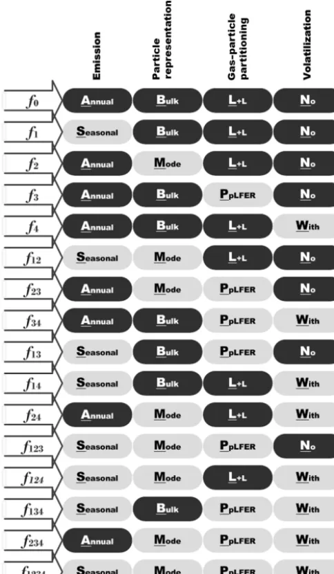
Factor separation analysis (Stein and Alpert, 1993) was used to quantitatively evaluate the contributions to changes in a particular output variable that result from changing com-ponents of model input and physics parameterizations. The model sensitivity to four model components (hereinafter, “factors”) was tested. The four factors were the following:
1. Temporal resolution of emissions (hereinafter, fac1).
The PAH emission inventory of Shen et al. (2013) was based on 2008 annual emission totals from all sectors (see Sect. 2.3.2). The emissions were divided over the year using monthly factors derived from BC anthro-pogenic emissions. Two sets of simulations were carried out to test the sensitivity of model output to the seasonal profile of emission. The first set used constant emissions throughout the simulations, whereas the second set used a monthly emission interval.
2. The size-discretization of particulate-phase PAHs (here-inafter, fac2). The two options for this factor were tested: bulk versus modal (Sect. 2.2.1). Note that with regards to BaP, 95 % of the emissions were assumed to be in particulate phase and for the modal-scheme sce-nario, all of the emitted particles are treated as the hy-drophobic Aitken (ki) tracers.
3. The choice of gas–particle partitioning scheme (here-inafter, fac3). The present study focuses on the com-parison between the Lohmann–Lammel and ppLFER schemes for gas–particle partitioning.
4. The influence of re-volatilization (hereinafter, fac4).
Model runs with the volatilization process switched off are compared to those runs which have volatilization switched on.
Figure 2.Locations of monitoring stations used in the study. The initial letter of each station ID refers to the individual monitoring network (E: EMEP and AMAP, D: DEFRA, I: IADN, M: MONET-Africa)
annual emission (A), the bulk scheme (B), the Lohmann– Lammel scheme (L), and no re-volatilization (N) were ap-plied. SMPW (i.e., Seasonal emission+ Modal scheme+ PpLFER scheme +With re-volatilization) is referred to as thetargetsimulation (f1234) in which the more sophisticated
choice of the four features (factors) was tested. The total (gas +particle) concentration at the lowest model level was se-lected for its higher relevance with all the factors (compared to, for example, atmospheric burden) and to facilitate direct comparison with observations.
3 Results and discussion 3.1 Sensitivity tests
The analysis of the factor separation results is given be-low. For each factor, the analysis includes the assessment of direct effects (fˆi) and total interaction effects (6fˆij+ 6fˆij k+ ˆf1234) on near-surface PAH concentrations in two
seasons, i.e., December–January–February (DJF) and June– July–August (JJA). Figure 4 shows the respective effects for all factors as relative to the seasonal means of the base ex-periment (f0). A positive value indicates a concentration
in-crease with respect to f0, whereas a negative indicates a
decrease. The spatial distributions off0andf1234seasonal
mean concentrations for the four species are shown in the Supplement Sect. SVI Figs. S4 and S5, respectively.
We studied the relative effects in five climate zones (Arc-tic, northern midlatitudes, the tropics, southern midlatitudes,
and Antarctica) The global distributions of the relative ef-fects are presented in Figs. S6–S13, whereas Figs. S14–S21 present the relative interaction effects from the individual combination of factors. In the following, we do not look to interpret concentration responses to each interaction term. The reasons for this are that (1) accounting for all such in-teractions is complicated given the number of factors and (2) higher-order interactions (combinations of more than two factors) are hard to physically interpret.
We further investigate the factor effects on model per-formance by comparing the predicted seasonal mean near-surface concentrations from 16 experiments against observa-tion data in the Arctic and northern midlatitudes (Supplement Sect. SVII).
3.1.1 Effects of seasonality of emissions
Figure 4a shows that using monthly emissions increases PAH concentrations in DJF and decreases the concentrations in JJA over the areas from the middle to high latitudes of the Northern Hemisphere (NH). This result is expected and is attributed to emissions during the northern winter (summer) being higher (lower) than annual means and photochemistry being less (more) active. Over the Arctic, the relative changes (fˆ1/f0) in DJF show a median increase of approx. 30 % for
PHE, PYR, and FLT, and 7 % for BaP, whereasfˆ1/f0in JJA
Figure 3.List of experiments performed for the factor separation analysis to study sensitivity to temporal variation in emission and process parameterizations (particulate-phase representation, gas– particle partitioning scheme, and volatilization); L+L: Lohmann– Lammel; PpLFER: poly-parameter linear free-energy relationships.
effect is more pronounced in the middle latitudes rather than in high latitudes (Supplement Sect. SVII, Fig. S22).
In general,fˆ1/f0becomes smaller over the northern
mid-latitudes by around half. The upper (lower) quartile offˆ1/f0
in DJF (JJA) indicates that about one-quarter of the areas of the temperate and polar regions experience an at least 40 % increase (decrease), most were located in northeastern Eura-sia (see the left panels of Figs. S6 and S7). Notefˆ1/f0over
the tropics are small to negligible (±1 %) mainly due to lit-tle variation in emissions from anthropogenic sectors. PAH concentrations may be higher in dry season due to increased amounts of biomass burning, but they are poorly represented
in the current inventory. In southern middle and high lati-tudes, the direct effects of emission change are substantially opposite in sign to the effects seen in the northern latitudes, being negative in DJF (median ranges from−4 % to−32 %) and positive in JJA (7 %–25 %).
The total interactions betweenfac1and other factors gen-erally produce opposite signals tofˆ1over middle and high
latitudes in the two seasons. This result indicates that the changes in other factors tend to buffer the influence of monthly emission on increasing or decreasingf0
concentra-tions. Some exceptions are seen over parts of East Asia in DJF for all species (Fig. S6, right panels) and over the South-ern Ocean in JJA for BaP (Fig. S7, right panels) where the interactions work to reinforce the direct effects. In DJF, the degree of interactions is smaller or comparable to the size offˆ1for the Arctic and northern midlatitudes but becomes
stronger by at least double for Antarctica. The opposite ten-dency is seen in JJA but only applies to PYR and FLT. In agreement tofˆ1, the interaction effects are less apparent over
the tropics. Note that the positive effects infˆ14 during local
summer tend to be more dominant than the effects in other combinations for PHE, PYR, and FLT (Figs. S18–S20). In the simulation, the presence of re-volatilization in summer tends to suppressfˆ1by promoting more gases available for
long-range transport, and thus implies a negative feedback. 3.1.2 Effects of size discretization of particulate-phase
tracer
The direct effects of the modal scheme (fˆ2) vary among
species (Fig. 4c).fˆ2is almost absent for PHE as the species
resides almost completely in the gas phase. For PYR and FLT,fˆ2 is negative during DJF over northern midlatitudes
(fˆ2/f0 quartiles range from−5 % to −30 %) and the
Arc-tic (−50 % to−75 %), whereas it is hardly visible in JJA or over other regions. Further analysis reveals stronger particle deposition results when the aerosol phase is discretized into different modes (not shown). In long-range transport under modal aerosol representation, the aerosols are more associ-ated with larger particles, hence particle deposition becomes more effective. The choice of size discretization has only mi-nor effects for atmospheric levels, except for BaP, especially during DJF, for which overestimates are significantly com-pensated for (Fig. S25). Actually, for BaP, the modal scheme generally decreases the concentrations in the Arctic (as me-dian, −35 % in DJF and −15 % during JJA) and increases (approx. 5 %) those over the mid- and low-latitude landmass (Figs. S8d and S9d, left panels).
Figure 4.Direct and interaction effects on seasonal-mean near-surface PAH concentrations of(a, b)monthly emissions (i=1),(c, d)the modal scheme (i=2),(e, f)the ppLFER scheme (i=3), and(g, h)volatilization (i=4). The direct effects(a, c, e, g)are expressed as the difference between two distributions (fˆi=fi−f0), whereas the interaction effects(b, d, f, h)are expressed as the sum of two (6fˆij,i6=j), three (6fˆ
ij k,i6=j6=k), and all (fˆ1234) factor interactions. They are presented as relative to concentrations from the base (f0) simulation.
from−20 % to−75 %) and in JJA (−6 % to−120 %). It is interesting to note that the interaction between the modal and ppLFER schemes has a major influence on the negative sig-nal (Figs. S15, S16, S19, S20), suggesting that the decrease in simulated concentration associated with the change from bulk to modal could be intensified when the ppLFER scheme is used. In the remaining areas, the interaction effects vary in sign spatially as illustrated in the right panels of Figs. S8b and c to S9b and c. Nevertheless, it shows for both species that maximum influences occur over the Southern Ocean in DJF (where the effects may reach 2 orders of magnitude) and midlatitude landmass in JJA (more than a factor of 5). As for BaP, the median effects are negative (−7 % to−30 %) in both seasons, although some positive signals are appar-ent in parts of high latitudes while the tropical oceans bear small synergistic effects. Similar to other species, the degree of interactions is stronger thanfˆ2by more than a factor of 3
for the majority of grid cells (Figs. S8d–S9d, right panels). The large fractions of the effects are dominated by 2-factor and 3-factor combinations related to the interaction with the ppLFER scheme and/or re-volatilization (Figs. S17, S21). 3.1.3 Effects of the choice of gas–particle partitioning
scheme
Figure 4e shows that the direct effects of the ppLFER scheme (fˆ3) show little spatial heterogeneities in both seasons and
for all species. The effects are barely important for PHE due to a low gas–aerosol partition constant (Kp);fˆ3 is positive
for PYR and FLT over polar regions and northern midlati-tudes especially in winter when low temperature favors par-titioning to aerosols (higherKp). The median offˆ3/f0varies
from 1 % to 25 % with some parts of Antarctica showing an increase larger than 50 %. For BaP, the effects are overall negative (by at least−5 %) withfˆ3/f0reflecting a positive
north–south gradient (increasing from the Arctic to Antarc-tica), associated in part with stronger signals over oceans (Figs. S10d and S11d, left panels). In particular under the modal size discretization, the choice of gas–particle parti-tioning scheme has only minor effects for atmospheric levels, except for BaP for which model overestimates are compen-sated by the choice of the ppLFER scheme (Fig. S25). Under the bulk size discretization, the ppLFER scheme tends to en-hance some of the overestimates in the Arctic summer (FLT, PYR; Figs. S23–S24). The application of ppLFER increases Kpas this module is calculated from not only interaction with
BC and OM (as in Lohmann–Lammel scheme) but also with some other aerosol matrices. HigherKpindicates higher
par-ticle mass fraction. For PYR and FLT, this leads to an in-crease in total atmospheric lifetime as the aerosol phase is not degraded, and can therefore be transported over a larger distance. For BaP, the additional particles are subject to de-positions and heterogeneous oxidation by ozone, particularly in regions away from sources. The factor influence is notably too small for PHE as oxidations occur in both phases.
The effects fromfac3interactions vary by region and are relatively stronger thanfˆ
3(Fig. 4f). This finding is common
to all species and seasons. The degree of effects is weaker for PHE compared to that for other species. However, the in-teractions increase polar concentrations in local summer by 20 % to a factor of 5, mainly associated with the coupled ef-fect of ppLFER and volatilization (fˆ34, Figs. S14 and S18).
For PYR and FLT, there is a high spatial variability over ex-tratropical regions in local summer, as indicated by the in-terquartile range (distance between the third and first quar-tiles). With regard to synergistic terms, ppLFER interactions with themodalscheme and re-volatilization, in 2- or 3-factor combinations, are more important than other contributions (Figs. S15–S16 and S19–S20). For BaP, the interaction ef-fects show negative signals similar tofˆ3, suggesting a
posi-tive feedback. The interactions exert a stronger influence on the concentrations of the oceans than on that of land, except in the tropics (Figs. S10d and S11d, right panels). The me-dian of relative effects ranges from−1 % to a factor of−10, minimum (maximum) in the northern (southern) extratrop-ics. Two second-order interactions likely make major contri-butions, i.e.,fˆ34 which dominates the response over oceans
andfˆ23which dominates over land (Figs. S17 and S21).
3.1.4 Effects of re-volatilization
The direct effects of re-volatilization (fˆ4) are illustrated in
Fig. 4g. fˆ4 is positive in the tropics in both seasons, with
the medianfˆ4/f0 ranging from 5 % to 50 %. Intensive
re-volatilization in this region would increase net surface fluxes, thereby increasing concentrations. For PHE, positivefˆ4
val-ues are more localized over the tropical landmass, whereas negative fˆ4 values are predicted over the tropical ocean
(Figs. S12a and S13a; left panels). The positive (negative) effects over land (ocean) areas are also apparent at higher lat-itudes during most of the year. This reflects the fact that the negative effects on concentrations over ocean act contrary to the positive effects on net surface fluxes, mainly caused by the nonlinear relationships of air–sea gas exchange (deposi-tion and volatiliza(deposi-tion), air and surface burden, atmospheric oxidation, and emissions. Accounting for re-volatilization compensates for a significant part of underestimates of PHE in the Arctic during summer, but adds to overestimates in midlatitudes (Fig. S22).
for≈60 % of PYR underestimation (Fig. S23) and explains most of, ≈60 %–80 %, the FLT overestimation (Fig. S24). For BaP, fˆ4is positive consistently across regions and
sea-sons (fˆ4/f0 ranges from 20 % to a factor of 10), with
sub-stantial effects occurring over oceans (Figs. S12d–S13d; left panels). Accounting for re-volatilization creates some over-estimates in the Arctic during summer (Fig. S25). It should be noted that the parameterization adopted here to describe volatilization from soils (the Smit scheme) is derived from an experimental study on mid-polar-to-polar pesticides and there is a need to validate and eventually sophisticate the pa-rameterization to apolar substances.
The interactions generally point toward positive effects for the high-to-medium volatility species (Fig. 4h), despite some negative effects present over parts of the southern (northern) oceans in DJF (JJA) (Figs. S12–S13; right panels). As for BaP, the effects are uniformly negative, inferring the interac-tions work in opposition to fˆ4. The negative response is
al-most entirely caused by the negativefˆ34, i.e., the 2-factor
in-teraction between re-volatilization and the ppLFER scheme (Figs. S17, S21). Compared tofˆ4, the degree of interactions
is weaker for PHE, except in polar regions during local sum-mer where the interactions could amplifyfˆ4. The above
im-plies that fˆ4 may point in the right direction regardless of
the influences from other factor changes. In contrast, the de-gree of interactions is overall comparable tofˆ4for the other
species.
3.2 Model evaluation
Model performance using the sophisticated realization of the four features (factors), i.e., Seasonal emission + Modal scheme +PpLFER scheme+With re-volatilization (SMPW), is presented below. Two predicted variables are evaluated, i.e., total (gas+particle) concentrations and aerosol particulate mass fraction at the lowest model level. The metrics applied are listed in the Supplement Sect. SV. 3.2.1 Near-surface air concentration
Firstly, the comparison to land monitoring stations is as fol-lows.
– Central tendency. Table 2 shows statistical indices for near-surface concentrations of atmospheric PAHs from observations and simulations and their comparisons, av-eraged across stations in the Arctic, northern midlati-tudes, and the tropics. We can see that observed mean concentrations are higher for PHE and smaller for BaP over all regions. Furthermore, the Arctic concentrations are lower than those in the northern midlatitudes by a factor of around 20 and those in the tropics by ap-prox. 2 orders of magnitude. The model captures well these species and regional variations, but the magni-tudes are both underestimated and overestimated. In the Arctic, it underestimates PHE (MB= −0.060 ng m−3)
and BaP (MB = −0.006 ng m−3) concentrations but slightly overestimates PYR (MB=0.001 ng m−3) and
FLT (MB=0.04 ng m−3). In the NH midlatitudes, the
model overestimates the three species predominantly occurring in the gas phase (MB=0.077–0.867 ng m−3) but underestimates BaP (MB= −0.58 ng m−3). Nega-tive bias is seen in the tropics for three PAHs (MB= −3.443 to−6.851 ng m−3). Nevertheless, the compari-son of model and observations at individual monitoring stations can be different from the regional mean statis-tics, as described in the Supplement Sect. SVIII. Com-paring all four PAHs, a larger degree of bias is found for BaP, which increases from the northern midlati-tudes (NMB= −0.58, NMBF= −1.40, FAC2=0.31, FAC10=0.79) to the Arctic (NMB = −0.92, NMBF = −12.17, FAC2=0.17, FAC10=0.33).
– Dispersion of monthly concentrations. In the following, the coefficient of variation (CoV) is used to compare the dispersion of concentrations among species of dif-ferent ranges. CoV was calculated by dividing the stan-dard deviation (SD) of all data points by its mean value (x). The observations show high variability (CoV>1) with CoV ranging between 1.12 and 2.14. The simu-lated concentrations appear to be less dispersed than the observations (CoV=0.78–1.93) except for the Arctic PHE and PYR concentrations. The degree of underes-timation is larger in the tropics with CoV being 30 %– 50 % smaller than the observations. Furthermore, corre-lations between predicted and observed concentrations are weaker than those in other regions wherer varies between 0.29 and 0.63 (the model reproduces 8 %–40 % of the variance in observed concentrations). Comparing the four species, the simulated BaP shows greater un-derpredictions of the variability where CoV values are less than half of those observed and correlations are less than 0.2 (accounting not over 4 % of observed variance). Higher variability in BaP measurements (than in model results) can be influenced by strongly varying emissions in source regions that are not reflected in the emission inventory (Matthias et al., 2009).
Figure 5.Seasonal mean total (gas+particle) concentrations of PAHs (ng m−3) from observations (solid lines) and simulations (dashed lines) averaged over all stations in the(a)Arctic,(b)northern midlatitudes, and(c)the tropics. Note that a logarithmic scale has been used for BaP concentrations in the Arctic.
Table 2.Statistics comparison of model simulation and observations of total (gas+particle) concentrations of PAHs from stations in the Arctic, northern midlatitudes, and the tropics.N: Number of observed-simulated monthly data pairs;x: mean; Q2x: median; SDx: standard deviation; GMx: geometric mean;x: simulated (M) or observed (O) data; MB: mean bias; RMSE: root mean square error; NMB: normalized mean bias; NMBF: normalized mean bias factor; FAC2: factor of 2; FAC10: factor of 10;r: correlation coefficient.
Arctic NH midlatitudes Tropics
Metrics Unit PHE PYR FLT BaP PHE PYR FLT BaP PHE PYR FLT
N months 89 89 89 46 361 328 372 405 34 34 34
N<LOQ months 0 0 0 30 0 0 0 0 0 0 0
O ng m−3 0.107 0.024 0.039 0.007 2.193 0.408 0.803 0.141 11.818 6.431 6.843 Q2O ng m−3 0.034 0.014 0.012 0.002 1.301 0.194 0.360 0.037 3.608 2.106 2.181
SDO ng m−3 0.162 0.027 0.054 0.015 2.956 0.582 1.135 0.253 16.598 10.141 10.217
GMO ng m−3 0.051 0.014 0.018 0.003 0.968 0.221 0.383 0.046 3.733 1.369 1.726
M ng m−3 0.046 0.025 0.079 5.2×10⁻⁴ 2.270 1.086 1.670 0.059 4.966 2.005 3.400 Q2M ng m−3 0.010 0.007 0.034 1.9×10⁻⁵ 0.840 0.500 0.736 0.022 4.274 1.236 2.012
SDM ng m−3 0.089 0.040 0.099 6.5×10⁻⁴ 2.955 1.225 2.007 0.085 3.897 2.019 3.462
GMM ng m−3 0:012 0.008 0.041 3.4×10⁻⁵ 1.144 0.635 0.913 0.028 2.816 1.038 1.788
MB ng m−3 −0.060 0.001 0.040 −0.006 0.077 0.679 0.867 −0.083 −6.851 −4.426 −3.443 RMSE ng m−3 0.118 0.038 0.099 0.016 3.564 1.404 2.383 0.279 16.005 10.631 10.392 NMB – −0.56 0.06 1.04 −0.92 0.04 1.66 1.08 −0.58 −0.58 −0.69 −0.50 NMBF – −1.30 0.06 1.04 −12.17 0.04 1.66 1.08 −1.40 −1.38 −2.21 −1.01
FAC2 – 0.20 0.28 0.30 0.17 0.40 0.39 0.30 0.31 0.26 0.23 0.29
FAC10 – 0.82 0.90 0.94 0.33 0.90 0.84 0.83 0.79 0.97 0.79 0.85
concentration is overestimated by up to a factor of 3 in summer while PYR is quite well predicted. In the NH midlatitudes, the model underestimates the amplitude but overestimates the concentrations of PHE, PYR, and FLT (by typically a factor of 2), whereas a systematic negative bias is found for BaP. In the tropics, both the amplitude and magnitude are too low in the model (for magnitude, by a factor of 2–5).
Additional findings are discussed in the Supplement Sect. SIX related to the comparison between EMAC model results and those from other global PAH modeling studies.
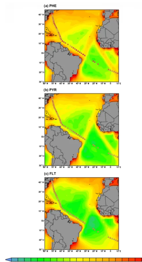
Secondly, the comparison to ship cruise measurements is as follows. Measurements of PHE, PYR, and FLT concentra-tions over the Atlantic Ocean were taken during a cruise in July 2009 (Lohmann et al., 2013). Figure 6 shows the ship sample concentrations overlaying the simulated PAH con-centrations. Sample arithmetic (geometric) means during the whole cruise transect are 322 (209), 95 (88), and 128 (111) pg m−3 for PHE, PYR, and FLT, respectively. The model poorly reproduces the remote marine environments and over-all underestimates the observations, except at 3 locations along the North American coast. The simulated means across sampling positions are 23 (7), 20 (3), and 39 (2) pg m−3, re-spectively, and the underestimation ranges from a factor of 2 to 1000. The degree of bias is most apparent over the tropical South Atlantic at latitude band 5–15◦S.
As reported in Liu et al. (2014), the measured concentra-tions of BaP over the Asian marginal seas, the Indian Ocean, the South Pacific Ocean, and North Pacific Ocean are 131 (45), 14 (3), 9 (2), and 8 (3) pg m−3, respectively, for the arithmetic (geometric) means of all samples. Similar to other species, the model also underestimates the BaP concentra-tions with mean values being 75 (15), 4 (0.05), 0.09 (0.03), and 0.2 (0.06) pg m−3, respectively. The discrepancy appears relatively smaller over the Asian marginal seas as compared to other locations (Fig. 7). A substantial degree of bias is seen over the Indian Ocean covering approximately the area bounded by 70–90◦E and 10–30◦S, with simulated values being more than 2 orders of magnitude smaller than the ob-served.
The model tendency to underestimate the marine air con-centrations may likely be due to several factors. (a) The grid resolution is not sufficient to reproduce fine-scale processes at the grid points close to shipping tracks; (b) high uncertain-ties associated with the air–sea gas exchange parameteriza-tions still exist, most notably in the estimation of gas transfer velocity; (c) the global inventory (Shen et al., 2013) may sig-nificantly underestimate emissions from ocean shipping and does not well characterize the spatial and temporal variabil-ity of biomass burning plumes as another potential point of origin of pollutants in the marine air (Nizzetto et al., 2008); and (d) PAH concentration over remote oceans is controlled by atmospheric components (e.g., temperature, wind speed, boundary layer height, photochemical degradation) and the
Figure 6. Simulated concentrations of PHE, PYR, and FLT (pg m−3) over the Atlantic ocean overlaid with concentrations from a ship cruise measurement campaign during July 2009 (triangles). Land grid cells are depicted in gray shades.
Figure 7.Simulated BaP concentrations (pg m−3) over the four ocean margins overlaid with concentrations from a ship cruise measurement campaign (triangles). Land grid cells are depicted in gray shades.
3.2.2 Particulate mass fraction
Measurements of particulate mass fraction (θ) were available only from the E3 station in Europe and IADN stations (I1–I7) in North America (see Table S11). Table 3 presents summary statistics on monthly mean θ from observations and simu-lations including some performance metrics. The observed mean θ is smaller for PHE (0.051±0.035) and higher for BaP (0.949±0.067). This result is expected as volatility de-creases (henceθ increases) from (lighter) PHE to (heavier) BaP. Theθvalues for PYR and FLT are larger by over 5 times than those for PHE and lower by around one-third than those for BaP. The model reproduces well the distinct differences among species but underestimates the observed θ for PHE, PYR, and FLT. The degree of negative bias is relatively large in PHE (NMB= −0.910 and NMBF= −10.145), whereas for the isomer pair of PYR and FLT, the model exhibits a similar performance with a slight improvement in PYR (NMB = −0.410 and NMBF = −0.694). With regard to BaP, there is a satisfactorily small bias (MB=0.015, RMSE =0.074, NMB=0.016, and NMBF=0.016) although the observed and simulated values have a very weak correlation (r=0.03).
Table 3.Statistics comparison of model simulation and observa-tions of particulate mass fraction (θ) from a subset of surface sta-tions, as listed in Table S11.N: Number of observed-simulated monthly data pairs;x: mean; SDx: standard deviation;x: simulated (M) or observed (O) data; MB: mean bias; RMSE: root mean square error; NMB: normalized mean bias; NMBF: normalized mean bias factor; FAC2: factor of 2; FAC10: factor of 10;r: correlation coef-ficient.
Metrics PHE PYR FLT BaP
N 63 63 99 93
O 0.051 0.359 0.268 0.949
SDO 0.035 0.150 0.162 0.067
M 0.005 0.212 0.106 0.964
SDM 0.005 0.138 0.086 0.027
MB −0.046 −0.147 −0.162 0.015 RMSE 0.057 0.214 0.225 0.074 NMB −0.910 −0.410 −0.604 0.016 NMBF −10.145 −0.694 −1.523 0.016
FAC2 0.00 0.56 0.30 1.00
FAC10 0.38 1.00 0.94 1.00
Figure 8.Seasonal mean particulate mass fraction (θ; unitless) from observations (solid lines) and simulations (dashed lines).
Figure 8 shows the seasonal meanθaveraged over 3 years for all PAHs. Observations show thatθ for BaP varies less than those for 3–4-ring PAHs. Although the model ade-quately reproduces this feature as well as seasonal variation of individual species, the simulatedθof PHE, PYR, and FLT is generally lower than the observations (except for PYR in winter). For BaP, differences between model and observa-tions are less than 10 % in all months. The SVOC submodel describes the gas–particle partitioning of atmospheric SOCs as a function of temperature and aerosol phase composition. The underestimation might be related to the fact that the sub-model assumes the particle to be fully in equilibrium with the gas phase at all times. It neglects kinetic limitations of molecular diffusivity that could lead to the trapping of par-ticles inside viscous (or semisolid) organic aerosol coatings. This shielding effect increases equilibration times of the par-ticles, thereby reducing part ofθfrom the mass available for gas–particle partitioning. Deviations from measurements can also be partly attributed to the locations of some stations that are within, or close to, residential and industrial area (namely I4, I6, and I7) where the scale and gradient in anthropogenic emissions are not resolved by the model grid resolution nor represented by the emission inventory.
4 Conclusions
The submodel SVOC has been developed and operated within the EMAC model for the application to global dis-tribution and environmental fate of SOCs. In this first de-velopment, the focus was set on the predictions of four PAH species: phenanthrene (PHE), pyrene (PYR), fluoran-thene (FLT), and benzo(a)pyrene (BaP). Multicompartmen-tal fate and air–surface exchange processes were included in SVOC. Some novel features in PAH modeling were tested, including seasonality in emissions, the modal scheme for particulate-phase tracer representation, the ppLFER scheme
for gas–particle partitioning, and re-volatilization from sur-faces. The results indicate that using seasonal emission com-pensates for model biases in the predictions of more volatile species (PHE), whereas the effects of the modal and ppLFER schemes are of less significance. Re-volatilization increases the near-ground concentrations in air, which is found most significant for species of mid semivolatility (PYR and FLT). The attribution of model response to individual features (fac-tors) is blurred by the nonlinear interactions between two or more factors. The effects of these interactions are found to both reinforce (positive feedback) and suppress (hence nega-tive feedback) the effects of the individual factors.
For near-surface concentrations, model bias varies by re-gion and/or species, being negative (positive) in the Arc-tic within typically a factor of 2–13 (6 % to a factor of 2) for PHE and BaP (PYR and FLT); positive in the northern midlatitudes for PHE, PYR, and FLT by up to a factor of 3; negative in the tropics (by a factor of 2–3); and largely over ocean up to 3 orders of magnitude. The model ade-quately reproduces the seasonal variation of the particulate mass fraction (θ), but underestimatesθfor high-to-medium-volatility PAHs. This might be related to a systematic under-estimation of OC by the model, which neglects secondary organic aerosols (SOA). The latter may cause significant un-derestimation of the overall atmospheric aerosol burden and θof SOCs, in particular over ocean. Since recently a MESSy submodel, ORACLE, dedicated to the simulations of SOA (Tsimpidi et al., 2014) based on lumping organic species in volatility bins is available. It should be included in future SOC simulations using EMAC.
Moreover, the implicit assumption of instantaneous gas– particle equilibrium for SVOC may cause both over- and un-derestimates ofθ, as interphase mass transfer my be kineti-cally limited to gaseous sources (hence overestimate ofθ) or within the particle bulk (hence underestimateθ), as the PAHs may become trapped within particles during transport (Fried-man et al., 2014; Zelenyuk et al., 2012; Mu et al., 2018). For multidecadal studies, the coupling of a 3-D ocean model (coupled with a marine biogeochemistry module) would be needed since the present model application does not allow for horizontal and vertical transports in the deep ocean. For the same reason, contaminant remobilization within deep soil layers should also be introduced. To this end, a multilayer (3-D) soil compartment would be needed to replace the 2-D soil compartment used here.
in-formation can be found at http://www.messy-interface.org (MESSy Consortium, 2018). The SVOC submodel will be incorporated into the next release version of the ECHAM/MESSy (EMAC) model (v2.55) and will therefore be made publicly available (with respect to the EMAC license regulations).
Supplement. The supplement related to this article is available on-line at: https://doi.org/10.5194/gmd-12-3585-2019-supplement.
Author contributions. MO and GL conceived the study and de-signed the experiments. MO developed the SVOC submodel with input from all co-authors. MO performed model simulations and data analyses. MO and GL discussed the results. MO wrote the ar-ticle with contributions from all co-authors.
Competing interests. The authors declare that they have no conflict of interest.
Acknowledgements. This study was supported by the Max Planck Institute for Chemistry. We thank the MESSy community and MESSy submodel developers for providing technical support. The model simulation was performed at the Max Planck Computing and Data Facility (MPCDF), Garching.
Financial support. The article processing charges for this open-access publication were covered by the Max Planck Society.
Review statement. This paper was edited by Havala Pye and re-viewed by two anonymous referees.
References
Batjes, N.: Total carbon and nitrogen in the soils of the world, Eur. J. Soil Sci., 47, 151–163, https://doi.org/10.1111/j.1365-2389.1996.tb01386.x, 1996.
Dalla Valle, M., Codato, E., and Marcomini, A.: Cli-mate change influence on POPs distribution and fate: A case study, Chemosphere, 67, 1287–1295, https://doi.org/10.1016/j.chemosphere.2006.12.028, 2007. Daly, G. L. and Wania, F.: Simulating the influence of snow on the
fate of organic compounds, Environ. Sci. Technol., 38, 4176– 4186, https://doi.org/10.1021/es035105r, 2004.
de Boyer Montégut, C., Madec, G., Fischer, A. S., Lazar, A., and Iudicone, D.: Mixed layer depth over the global ocean: An examination of profile data and a profile-based climatology, J. Geophys. Res.-Oceans, 109, C12003, https://doi.org/10.1029/2004JC002378, 2004.
Dee, D. P., Uppala, S. M., Simmons, A. J., Berrisford, P., Poli, P., Kobayashi, S., Andrae, U., Balmaseda, M. A., Balsamo, G., Bauer, P., Bechtold, P., Beljaars, A. C. M., van de Berg, L., Bid-lot, J., Bormann, N., Delsol, C., Dragani, R., Fuentes, M., Geer,
A. J., Haimberger, L., Healy, S. B., Hersbach, H., Hólm, E. V., Isaksen, L., Kållberg, P., Köhler, M., Matricardi, M., McNally, A. P., Monge-Sanz, B. M., Morcrette, J.-J., Park, B.-K., Peubey, C., de Rosnay, P., Tavolato, C., Thépaut, J.-N., and Vitart, F.: The ERA−Interim reanalysis: configuration and performance of the data assimilation system, Q. J. Roy. Meteor. Soc., 137, 553–597, https://doi.org/10.1002/qj.828, 2011.
DEFRA: UK Department of Environment, Food and Rural Af-fairs, Polycyclic Aromatic Hydrocarbons (PAH) data, available at: https://uk-air.defra.gov.uk/data/pah-data (last access: 15 Au-gust 2017), 2010.
Dunne, K. A. and Willmott, C. J.: Global distribution of plant-extractable water capacity of soil, Int. J. Clima-tol., 16, 841–859, https://doi.org/10.1002/(SICI)1097-0088(199608)16:8<841::AID-JOC60>3.0.CO;2-8, 1996. Endo, S. and Goss, K.-U.: Applications of polyparameter linear free
energy relationships in environmental chemistry, Environ. Sci. Technol., 48, 12477–12491, https://doi.org/10.1021/es503369t, 2014.
European Commission: Guidance document on persistence in soil, Technical Report 9188/VI/97 in relation to Council Directive No. 97/57/EC, EC Directorate General for Agriculture, 2000. Finizio, A., Mackay, D., Bidleman, T., and Harner, T.: Octanol−air
partition coefficient as a predictor of partitioning of semi-volatile organic chemicals to aerosols, Atmos. Environ., 31, 2289–2296, https://doi.org/10.1016/S1352-2310(97)00013-7, 1997. Friedman, C. L. and Selin, N. E.: Long-range atmospheric transport
of polycyclic aromatic hydrocarbons: global 3-D model analysis including evaluation of Arctic sources, Environ. Sci. Technol., 46, 9501–9510, https://doi.org/10.1021/es301904d, 2012. Friedman, C. L., Pierce, J. R., and Selin, N. E.: Assessing the
influence of secondary organic versus primary carbonaceous aerosols on long-range atmospheric polycyclic aromatic hy-drocarbon transport, Environ. Sci. Technol., 48, 3293–3302, https://doi.org/10.1021/es405219r, 2014.
Galarneau, E., Makar, P. A., Zheng, Q., Narayan, J., Zhang, J., Moran, M. D., Bari, M. A., Pathela, S., Chen, A., and Chlum-sky, R.: PAH concentrations simulated with the AURAMS-PAH chemical transport model over Canada and the USA, At-mos. Chem. Phys., 14, 4065–4077, https://doi.org/10.5194/acp-14-4065-2014, 2014.
Gantt, B., Meskhidze, N., Facchini, M. C., Rinaldi, M., Ce-burnis, D., and O’Dowd, C. D.: Wind speed dependent size-resolved parameterization for the organic mass fraction of sea spray aerosol, Atmos. Chem. Phys., 11, 8777–8790, https://doi.org/10.5194/acp-11-8777-2011, 2011.
Gong, S. L., Huang, P., Zhao, T. L., Sahsuvar, L., Barrie, L. A., Kaminski, J. W., Li, Y. F., and Niu, T.: GEM/POPs: a global 3-D dynamic model for semi-volatile persistent organic pollutants – Part 1: Model description and evaluations of air concentrations, Atmos. Chem. Phys., 7, 4001–4013, https://doi.org/10.5194/acp-7-4001-2007, 2007.
Goss, K.-U. and Schwarzenbach, R. P.: Linear free en-ergy relationships used to evaluate equilibrium partition-ing of organic compounds, Environ. Sci. Technol., 35, 1–9, https://doi.org/10.1021/es000996d, 2001.