Evaluating performance of meta-heuristic algorithms and decision tree models in simulating water level variations of dams’ piezometers

Journal of Hydraulic Structures

J. Hydraul. Struct., 2018; 4(2):60-80 DOI: 10.22055/jhs.2018.27833.1092

Evaluating performance of meta-heuristic algorithms and

decision tree models in simulating water level variations of

dams’ piezometers

Rezvan Salajegheh1 Amin Mahdavi-Meymand2 Mohammad Zounemat-Kermani3

Abstract

Monitoring the seepage, particularly the piezometric water level in the dams, is of special importance in hydraulic engineering. In the present study, piezometric water levels in three observation piezometers at the left bank of Jiroft Dam structure (located in Kerman province, Iran) were simulated using soft computing techniques and then compared using the measured data. For this purpose, the input data, including inflow, evaporation, reservoir water level, sluice gate outflow, outflow, dam total outflow, and piezometric water level, were used. Modeling was performed using multiple linear regression method as well as soft computing methods including regression decision tree, classification decision tree, and three types of artificial neural networks (with Levenberg-Marquardt, particle swarm optimization, PSO, and harmony search learning algorithms, HS). The results of the present study indicated no absolute superiority for any of the methods over others. For the first piezometer the ANN-PSO indicates better performance (correlation coefficient, R=0.990). For the second piezometer ANN-PSO shows better results with R=0.945. For the third piezometers MLR with R=0.945 and ANN-HS with R=0.949 indicate better performance than other methods. Furthermore, Mann-Whitney statistical analysis at confidence levels of 95% and 99% indicated no significant difference in terms of the performance of the applied models used in this study.

Keywords: Data driven models; dam surveillance; soft computing, heuristic algorithms, dam engineering.

Received: 8 December 2018; Accepted: 26 December 2018

1. Introduction

Seepage is one of the major issues in various engineering levees and dams, so that in most of

1 _{Department of Civil Engineering, Baft Branch, Islamic Azad University, Baft, Iran.} 2 _{Department of Water Engineering, Shahid Bahonar University of Kerman, Kerman, Iran}

the cases, the problems related to these structures are associated, either directly or indirectly, with seepage; therefore, monitoring and identifying the seepage behavior play important role in the safety and security of the engineering levees and dams [1-3]. Piezometric devices installed and used in certain sections of the dam to measure the seepage based on water level. In relation to monitoring and investigating the issue of seepage, numerous studies have been conducted to date, most of which have been focused on investigating the seepage rate and seepage monitoring in different sections of dams [4]. Although concrete dams are considered impenetrable, they have been encountering serious seepage-related problems due to their specific construction conditions [2]. In practice, in order to monitor seepage, some piezometers are improvised in certain parts of the dam [5, 6].

In addition, some other physical methods (drilling boreholes and using dye trace test) as well mathematical models and numerical methods can be also used to identify the seepage path and solve the seepage path problems [7].

In recent decades, regarding the successful application of data-based methods for simulating various kinds of engineering problems, the soft computing methods have been widely used for solving the dam engineering problems. Several studies have evaluated the performance of these methods in predicting the dam location variation, dam section optimization, and fracture in arch dams [1].

In order to predict water level in piezometers, Tayfur et al. [8] used ANN, and considered the upstream and downstream water levels as the input data. Gholizadeh and Seyedpoor [9] used neural network and PSO (particle swarm optimization) and GA (genetic algorithm) to show the impact and importance of soft computing in achieving the optimal arch dam design geometry, which can provide stability of the dam against natural pressures.

Zhou et al. [5] used a compound method, consisted of orthogonal design (OD), ANN, FE, and GA, for modelling the leakage and seepage problems. Zhou et al. [5] used BPNN (back-propagation neural network) to depict the implicit map of environmental parameters in order to investigate the impermanent seepage flow's response at dam monitoring points. Stojanovic et al. [10] presented a self-tuning system for dam behavior modelling based on ANN with genetic algorithm (ANN/GA) compared to MLR, the results of which implied superiority of the ANN-GA method over other methods. Xiang et al. [4] used PSO algorithm to optimize the seepage model parameters, the results of which indicated the higher precision and accuracy of this method compared to previous statistical methods.

Nourani et al. [11] used neural network and ANFIS (adaptive network-based fuzzy interference system) to investigate contamination concentration over time in porous environments. Studies have shown that the complexity of the underground water flow and transmission of contamination have caused the use of black box methods, such as neural networks and ANFIS.

The present study is aimed to simulate the water level in piezometers of Jiroft double-curvature arch dam in Kerman province, Iran, using three samples of MLP artificial neural networks (with Levenberg-Marquardt training algorithm as well as PSO and HS algorithms), and to compare the results obtained from the MLR, classification decision tree, and regression decision tree methods. To best of the authors’ knowledge, assessing the performance of classification regression tree, regression decision tree, ANN-PSO and ANN-HS to predicting the water level in piezometers has not been studied in past researches. Hence, the application of these soft computing models is the novelty and the contribution of this study.

2. Materials and methods

2.1. Case study and dataset

Jiroft dam is a double-curvature arch concrete dam operated in 1991, which is located in the study zone of Hamun-e-Jaz Murian at the central basin and is fed by Halilriver in the northeast of the Jiroft city in the narrow valley of Narab (Figure 1). This dam has been constructed with the aim of generating electricity and supplying the water requirement of agricultural and environmental sectors; besides, it is also used as a secondary target for supplying drinking water. The electricity generation capacity of this dam is 80 GW, and it features reservoir volume of 336 m3, dam height of 128 m, height above its foundation of 132 m, crest length of 250 m, and lake length of 12 km; also, the spillway is of middle and surface sluice type [12].

(a) (b)

Figure 1. (a) Aerial image of Jiroft double-curvature arch concrete dam in Kerman province, Iran; (b) Schematic image of cross section of dam and location of piezometers used in this study, which

are situated at left bank retain wall in the body and rock (rock is the foundation) of the dam.

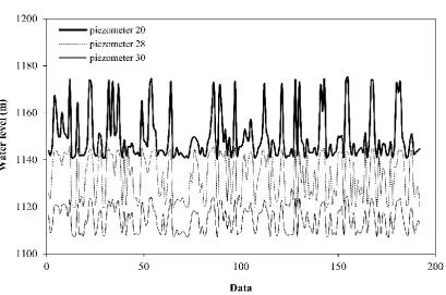
Figure 2. Historical variations of water level in the three studied piezometers in this research.

Figure 2 shows the historical variations of water level in the three piezometers. As could be expected from the location of piezometers (see Figure 1), the average values of surface water level in Piezometer 20 is more than the other two piezometers. Also total variations in Piezometer 28 is less than the other two piezometers. In this study the hold-out method is used as the method of sampling. In this respect, datasets are divided into two categories of training (80%) and testing (20%) phases for modelling implementation. Training data are used for the learning process of the models, while testing data are used to evaluate the performance of the models. A summary of the statistical characteristics of the measurement data of the output vector (reservoir water level variations) and input vector is provided in Tables (1) and (2).

Table 1- Statistical analysis of piezometers’ water level data used in the present study

SK CV

SD Ave (m)

Min (m) Max (m)

Piezometer

1.472 0.008

10.235 1149.657

1140.9 1175.1

20

-0.150 0.00

9.442 1132.954

1119.84 1145.55

28

0.175 0.004

5.473 1114.459

1107.07 1124.48

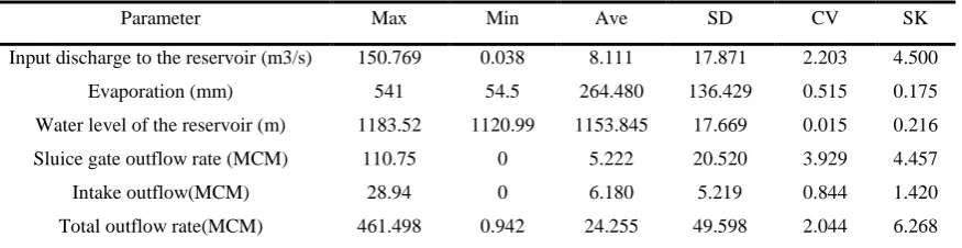
Table 2 - Statistical analysis of input parameters of data driven models SK CV SD Ave Min Max Parameter 4.500 2.203 17.871 8.111 0.038 150.769

Input discharge to the reservoir (m3/s)

0.175 0.515 136.429 264.480 54.5 541 Evaporation (mm) 0.216 0.015 17.669 1153.845 1120.99 1183.52

Water level of the reservoir (m)

4.457 3.929 20.520 5.222 0 110.75

Sluice gate outflow rate (MCM)

1.420 0.844 5.219 6.180 0 28.94 Intake outflow(MCM) 6.268 2.044 49.598 24.255 0.942 461.498

Total outflow rate(MCM)

2.2 Data driven models used in this study

2.2.1 MLR model

Multiple (multivariate) linear regression is a method in which two or more independent variables contribute to the variations of a variable, and is one of the most effective prediction methods; thus, it is widely used in researches that are aimed to investigate and predict a specific phenomenon. In such researches, regarding the independent variables, a regression relation is extracted, based on which the dependent variable is predicted. The general form of the equation is as follows [1, 10]:

0 1 1 2 2 N N

WLβ β u β u β u (1)

where, WL stands for the piezometer’s water level (dependent parameter) and βi represents coefficients of the independent parameters and is estimated by sum of square error, and ui indicates the input variable vector [13].

2.2.3 Decision tree models

A decision tree represents a structure in which the leaves indicate classes (categories), and the branches indicate combinations of the attributes resulting in these classes. Decision trees classify the samples by sorting them in the tree from the root toward leaf nodes. Each internal node in the tree tests an attribute of the sample, and each branch coming out of that node corresponds to a possible value for that attribute. Each leaf node represents a class. Each sample begins from the root and after testing the attribute in this node, moves in the corresponding branch with regard to the attribute, and finally is placed in an appropriate class. This process is repeated regressively for each sub tree. The regression is completed when further separation is not useful anymore or a classification cannot be applied to all the samples existing in the obtained subset [14, 15].

Decision trees are capable to generate attributes from the relations in a dataset, which are perceivable for human and can be used for classification and prediction. Decision trees are divided into four main groups, including classification trees, regression trees, classification-regression trees, and cluster trees. In the present study, two types of these trees, namely classification and regression trees are used [15-17].

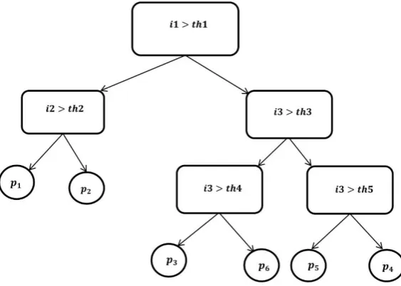
2.2.3.1 Regression decision tree (RDT)

The output of a medium decision tree is the observed output variable in each group. When there is more than one predictor, the best separator (distinction) point is calculated for each of them, and the factor resulting in the highest error reduction rate is selected; therefore, the inappropriate (irrelevant) predictors are automatically eliminated by the algorithm, so that error reduction for a separator in a low-importance predictor will be generally less than that in a more useful one. Other dominant characteristics of the regression decision trees include [17] : they are robust against outliers, require little data preprocessing, can handle numerical and categorical predictors, and are appropriate for modelling nonlinear relations, as well as interaction among predictors.

Figure 3. Schema of structure of a regression decision tree

Figure 3 shows a profile of a regression decision tree [15] . In order to improve precision of prediction, it calculates the re-substitution error, test sample error, and cross-validation error. The error is estimated by applying the data used for determining the structure of the predictor p and is calculated as the MSE (mean square error).

 



 



i i

i 1

1

E p u p v

N 





Where, (ui, vi) indicates training samples, and i=1,2,3,…,N is divided into K subsamples in order to estimate the re-substitution error of sample X with size of N. Also, X1,X2,…,XK with approximate size of N1,N2,…NK from X-XK subsamples are used for making the predictor p. Finally, this error of the sample XK is calculated using the following formula:

 

 

 

_{ }





1

i i k

k cv

i i

k u v x

k

E

P

v

p

u

N



 



 

  2





2

2

1

i i

N ts

i ui

u v X

E

p

v

p

N







where, x2 is a subsample that is not used in the prediction structure.

Finally, the output of each decision tree is calculated via the following formula:

 

_{ }



 



i i i

i t w

R t w f u v t N t _





Where, Nw(t) is the weight of data at t, wi is the value of the weighting variable for case i, fi is the value of the frequency variable, vi is the value of the response variable, and v

-(t) is the weighted mean for node t.

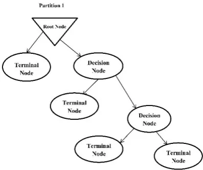
2.2.3.2 Classification decision tree (CDT)

Classification decision trees are used to predict discrete data (Figure 4). In order to have a better classification tree, the classification process must have error freedom as much as possible. This means that final nodes of the tree should be as homogenous as possible regarding the predicted variable. For this purpose, a step-wise algorithm creates an optimal classification of the training data, in which both categorical and prediction variables are known and clear. At each step, all of the possible branches are tested and compared based on each explanatory variable. And finally, the selected branch introduces the optimal subset [16, 18, 19].

Figure 4. Schema of a classification decision tree

2 1 N i split i i N GINI GINI 









1

1

GINI

p







Where, GINIi is the GINI index of the child node i, Ni is the number of samples at the child node i, N is the number of samples at the parent node, Pj is the probability of class j at node i, and k is the number of classes.

2.2.3 Artificial neural networks (ANNs)

ANNs, with considerable ignorance, can be called the electronic models of the human brain's neural structure. In fact, the aim of creating a software neural network is, rather than simulating the human brain, to create a mechanism for solving the engineering problems inspired by the behavioral pattern of biological networks. These networks are capable to distinguish between the input patterns; thus, they can be used in a wide range of complex problems, including recognition of patterns, nonlinear models, classifications, etc. ANNs are divided into two main groups, namely recurrent networks, in which the loop occurs, and feed-forward neural networks, the structure of which lacks loops. Selecting the network's structure depends on the learning algorithm used for training of the network. A specific type of neural networks, known as FNN 3-layer neural network, has been widely used for solving many of the civil engineering and water engineering problems[1 , 20].

2.2.3.1 Back propagation feed forward neural network

There are various types of neural networks, the most important of which is the back propagation feed forward neural networks (BPFNN). Similar to other types of neural network, FNNs are composed of simple components, which are called neurons. Neurons are located in layers, and neurons of the adjacent layers are interconnected to each other via connectors of an independent unit (synapses), which transfer the information from one neuron to other ones. The input data are stored in neurons of the first layer (input layer), and the outputs are displayed by neurons of the last layer (output layer). All the layer located between the input and output layers are known as the hidden layers (Honric, 1991).

The activation function is associated with layers, and its role is to scale and classify the output data of the layers. The most common types of activation functions include linear and sigmoid types. The linear activation functions are represented by the following general form:

 

f y



y

Two common types of sigmoid activation functions, which are used in these networks, include hyperbolic tangent function and logistic function.

 

1

0

1

f

e





 

 (10)

Output =

f y

 

Where 1 k

i i

i

y w x b







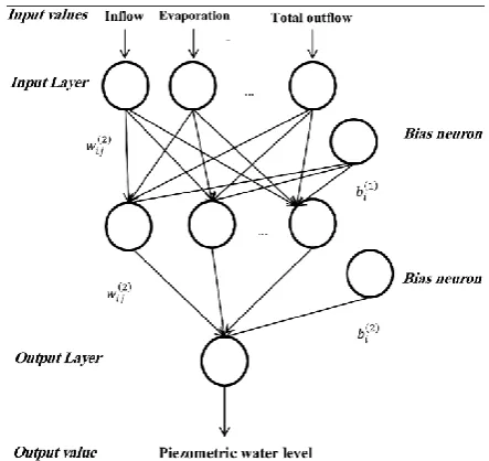
and b is the bias component. Figure (5) shows an FNN with 3 layers and S neurons in the input layer. The inputs are x=(x1,x2,…xk), which are collected at the hidden nodes along with weights. At the nodes, first, the signal is collected and then a nonlinear function is applied (e.g. hyperbolic tangent); finally, the output y appears under a linear function at the output nodes.

Figure 5. Three-layer neural network used in the present study

 

   

 

1 1

1

2 2

( )

1

1

1

s i ij i j

k

ij i

x w b

i

y

w

b

e













where, s is the number of inputs, k is the number of hidden neurons, xj indicates j input elements,

𝑤_𝑖𝑗(1) is the weight of the first layers between i hidden neurons and j inputs, 𝑤_𝑖𝑗(2) is the weight of

the second layer between i hidden neurons and the output neuron, 𝑏_𝑖(1) is the base weight for i

hidden neurons, and 𝑏_𝑖(2) is the base weight for the output neurons [1,21].

2.2.4 Optimization methods

Optimization is indeed a method for utilizing the linear and nonlinear capability of the formulas in order to solve a wide range of problems and analyze the solutions [22]. In the present study, in order to optimize the weight values of the neurons of the ANN, the Levenberg-Marquardt mathematical optimization method as well as PSO and HS meta-heuristic optimization methods was used.

2.2.4.1 Levenberg-Marquardt mathematical algorithm

function, which is used as a standard method for solving the least square problem for nonlinear functions. It is widely used in FNNs in order for reducing the errors by point reduction of the error curve's slope [23-25].

Due to its effective role in accurate calculation of the weights' error, this algorithm has been considered and investigated as the most well-known and prominent training structure, and is currently used for generalizing the delta role (variations) in nonlinear activation functions and multi-layer networks. In Marquardt algorithm, the error function is minimized, while the size of the computational steps is small; accordingly, in order to reassure accuracy of the linear approximations, this objective was accomplished by the following modified error function [22].

 









2 2

1

1 2

ek

j j j j j

wi

E _e  w _ w _ 





  (13)

Where,  is the parameter representing the step size, the minimum error, with regard to w(j+1) is expressed as following:

 1  





T T

j

j j

W



W



Z Z





I Z e

High values of  cause declination of the standard gradient, and its lower value inclines toward Newton method.

2.2.4.2 PSO algorithm

PSO algorithm was created by Kennedy & Eberhart [26] based on the collective movement of birds or a group of fish. PSO is an optimization sample capable to model the human population for processing the science, which is rooted in two main components of methodology, namely artificial life (such as groups of birds, schools of fish) and evolutionary counting (evolutionary computations). PSO algorithm is based on the assumption of the potential of movement in a space full of high-speed particles toward the optimal solution. It is a populated search method for optimizing the nonlinear functions [27] Furthermore, PSO extracts the best cooperation status, and uses it for optimizing the engineering problems. The particles simply follow the set of predetermined roles. PSO calculates the particles based on the performance capability, and then selects the particle with the best solution. The particle with best capability is selected as the trainer; subsequently, all the particles are trained by the selected particles. No two particles are similar, and instead they utilize other particles' attributes to improve their own performance [28].

For each particle, two values of position and speed is defined, which are modeled by a location vector and a speed vector, respectively. These particles move repeatedly in the n-dimensional space of the problem. Dimensions of the problem are determined by the number of parameters of the problems. The general form of the algorithm's equation is represented below [29]:



1



 



 

 





 

 



ij ij ij ij gi ij

v t



 

wv t





c



p t





x t





c



p

t





x t





1



 



1



ij ij ij

x t



 

x t





v t





𝑣_𝑖𝑗 ∈ [−𝑣_𝑚𝑎𝑥. 𝑣_𝑚𝑎𝑥], and if the search space is limited to [−𝑥_𝑚𝑎𝑥. 𝑥_𝑚𝑎𝑥], then 𝑣_𝑚𝑎𝑥 = 𝑘𝑥_𝑚𝑎𝑥 with 0.1 ≤ k ≤ 1. Also, 𝑝_𝑖𝑗(𝑡́) − 𝑥𝑖𝑗(𝑡́) represents the distance between the current location and

optimal location of the ith particle, and 𝑝_𝑖𝑗(𝑡́) − 𝑥_𝑖𝑗(𝑡́) indicates the distance between the current location and the optimal location of the ith particle in the group.

2.2.4.3 HS (harmony search) algorithm

Harmony search, which is a heuristic algorithm imitating the musicians' structure for finding the best harmony, is widely used for solving the complex problems that cannot be solved by old methods. It has several advantages over previous optimization methods. It applies the last absolute mathematical features such as differentiability, continuity, and convexity [30]. According to the definition presented by Geem et al. [31], the HS algorithm is based on the minimum mathematical requirements and begins from probable random search; therefore, it does not require much secondary information. The vector introduces the final solution with regard to all the resulted vectors.

In HS algorithm, the musician looks for the best harmony that has been arranged aesthetically. Accordingly, the optimizer algorithms look for the best status with regard to the objective function. Each musician is associated with the decision variable, and the musical instruments' beats are sorted based on the importance of the decision variable. The musical harmony at a certain time is associated with the leader vector in a certain repetition. The hearer's enjoyment is the final objective (output of the harmony). Furthermore, just like the stepwise improvement of the musical harmony, the solution vector in the algorithm moves toward the optimal solution in each repetition [32].

Each musician has three options: (1) playing each pitch based on his own memory, (2) playing something similar to the given music, and (3) playing a new or random note. These explanations are generally expressed by the following formula [33]:



2

1



new old p

x



x



b



rand



 

 



 

 



x i



x

i



x

i



x

i



rand

Where, xnew is the new solution after a certain beat, xold is the solution from memory of harmony,

𝑟𝑎𝑛𝑑 ∈ [0,1], bp is the bandwidth vector, i is equal to 3, and xmin(i) and xmax(i) are the minimum and maximum values of i, respectively.

3. Implementing and executing the model

3.1 Preparing data

3.2 Evaluating model’s performance

In the present study, in order for evaluating the performance of the used models, several statistical indices, including MSE (mean square error), MAE (mean absolute error), and RMSE (root mean square error), and correlation coefficient (R) were used.















y

y

m

m

R

y

y

m

m

  





















1

i i

i O

MSE

y

m

N







O N i i i 1 O

1

MAE

y

m

N











1

RMSE

y

m

N







where, yi and mi represent the network's output and measured data for i elements, respectively, and y̅ and m̅ represent the mean of parameters, and NO indicates the number of them.

3.3 Setting up the models

In the present study, in order to predict the water level in piezometers 20, 28, and 30, the 3-layer neural network, regression decision tree, classification decision tree, and multivariate linear regression were used. Precision of any model is directly dependent on the input parameters; therefore, the input parameters included the monthly gathered data, including: evaporation, inflow, reservoir water level, sluice gate outflow, outflow, dam total outflow, and read water level of piezometers. The training data were considered as the basis of modelling for all the models. In order for modelling using neural networks, several neural networks with different architectures were taken into consideration. By considering different numbers of neurons in the network, the best state of the network was identified. Finally, by considering three neurons in the middle layer, the intended neural network was built, and performance of different transmission functions was compared. The neural network's parameters (weights and biases) were optimized using LM, PSO and HS algorithms. By initiating the weights and biases, the final values of these coefficients were extracted using the above-mentioned algorithms, and then these extracted values were used for modelling the neural network. The results obtained for different transmission function, considering three neurons in the middle layer, were evaluated so that these methods can be compared in the same conditions. In order for modelling via classification and regression decision trees, the intended models were constructed using the training data as the inputs; then, the performance of these models was evaluated using the test data.

4. Results and discussion

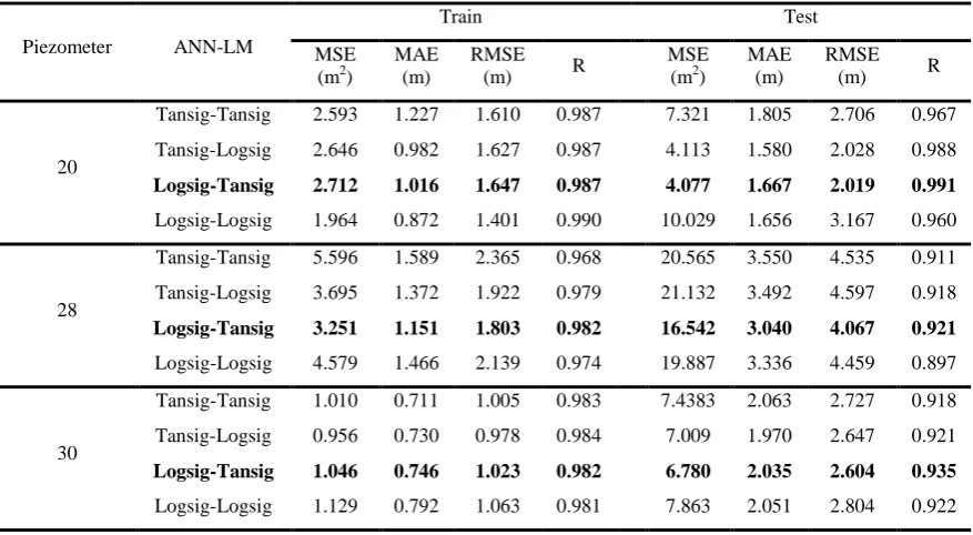
Table 3- Results of modelling ANN-LM in order to simulate water level variations of piezometers of Jiroft Dam

Piezometer ANN-LM

Train Test

MSE (m2)

MAE (m)

RMSE

(m) R

MSE (m2)

MAE (m)

RMSE

(m) R

20

Tansig-Tansig 2.593 1.227 1.610 0.987 7.321 1.805 2.706 0.967

Tansig-Logsig 2.646 0.982 1.627 0.987 4.113 1.580 2.028 0.988

Logsig-Tansig 2.712 1.016 1.647 0.987 4.077 1.667 2.019 0.991

Logsig-Logsig 1.964 0.872 1.401 0.990 10.029 1.656 3.167 0.960

28

Tansig-Tansig 5.596 1.589 2.365 0.968 20.565 3.550 4.535 0.911

Tansig-Logsig 3.695 1.372 1.922 0.979 21.132 3.492 4.597 0.918

Logsig-Tansig 3.251 1.151 1.803 0.982 16.542 3.040 4.067 0.921

Logsig-Logsig 4.579 1.466 2.139 0.974 19.887 3.336 4.459 0.897

30

Tansig-Tansig 1.010 0.711 1.005 0.983 7.4383 2.063 2.727 0.918

Tansig-Logsig 0.956 0.730 0.978 0.984 7.009 1.970 2.647 0.921

Logsig-Tansig 1.046 0.746 1.023 0.982 6.780 2.035 2.604 0.935

Logsig-Logsig 1.129 0.792 1.063 0.981 7.863 2.051 2.804 0.922

Table 4- Results of combining ANN-PSO in order to simulate water level variations of piezometers of Jiroft Dam

Piezometer ANN-PSO

Train Test

MSE (m2)

MAE (m)

RMSE

(m) R

MSE (m2)

MAE (m)

RMSE

(m) R

20

Tansig-Tansig 4.926 1.567 2.219 0.976 3.614 1.494 1.901 0.991

Tansig-Logsig 4.621 1.300 2.149 0.977 2.533 1.194 1.592 0.990

Logsig-Tansig 9.422 2.275 3.069 0.953 8.796 2.355 2.966 0.974

Logsig-Logsig 4.739 1.457 2.177 0.977 3.965 1.477 1.991 0.992

28

Tansig-Tansig 4.599 1.421 2.145 0.974 13.455 2.898 3.668 0.938

Tansig-Logsig 4.721 1.473 2.173 0.973 16.013 3.105 4.002 0.913

Logsig-Tansig 5.701 1.656 2.387 0.968 14.379 3.090 3.792 0.930

Logsig-Logsig 5.611 1.511 2.369 0.968 11.549 2.736 3.398 0.945

30

Tansig-Tansig 3.475 1.424 1.864 0.956 3.253 1.374 1.803 0.948

Tansig-Logsig 3.505 1.486 1.872 0.943 3.626 1.432 1.904 0.942

Logsig-Tansig 3.043 1.389 1.745 0.949 3.412 1.444 1.847 0.945

Logsig-Logsig 2.922 1.361 1.709 0.952 3.329 1.386 1.824 0.948

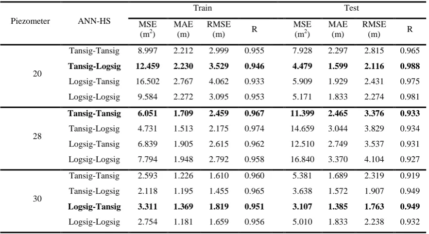
Table 5- Results of combining ANN-HS in order to simulate water level variations of piezometers of Jiroft Dam

Piezometer ANN-HS

Train Test

MSE (m2)

MAE (m)

RMSE

(m) R

MSE (m2)

MAE (m)

RMSE

(m) R

20

Tansig-Tansig 8.997 2.212 2.999 0.955 7.928 2.297 2.815 0.965

Tansig-Logsig 12.459 2.230 3.529 0.946 4.479 1.599 2.116 0.988

Logsig-Tansig 16.502 2.767 4.062 0.933 5.909 1.929 2.431 0.975

Logsig-Logsig 9.584 2.272 3.095 0.953 5.171 1.833 2.274 0.981

28

Tansig-Tansig 6.051 1.709 2.459 0.967 11.399 2.465 3.376 0.933

Tansig-Logsig 4.731 1.513 2.175 0.974 14.659 3.044 3.829 0.934

Logsig-Tansig 6.839 1.905 2.615 0.962 12.510 2.749 3.537 0.931

Logsig-Logsig 7.794 1.948 2.792 0.958 16.840 3.370 4.104 0.927

30

Tansig-Tansig 2.593 1.226 1.610 0.960 5.381 1.689 2.319 0.919

Tansig-Logsig 2.118 1.195 1.455 0.965 3.638 1.572 1.907 0.949

Logsig-Tansig 3.311 1.369 1.819 0.951 3.107 1.385 1.763 0.949

Logsig-Logsig 2.754 1.181 1.659 0.956 5.010 1.833 2.238 0.932

concluded that the regression decision tree had the best performance for all three piezometers (Table 6).

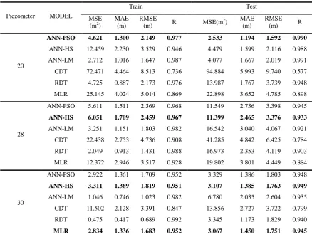
The results obtained from all methods are summarized in Table (6). The results shown for all methods calculated statistical parameters are at the suitable level, which implies that all soft computing technics predict water levels with high accuracy.

Table 6- Comparing the performance of all the applied methods used in this study

Piezometer MODEL

Train Test

MSE (m2)

MAE (m)

RMSE

(m) R MSE(m

2₎ MAE

(m)

RMSE

(m) R

20

ANN-PSO 4.621 1.300 2.149 0.977 2.533 1.194 1.592 0.990

ANN-HS 12.459 2.230 3.529 0.946 4.479 1.599 2.116 0.988

ANN-LM 2.712 1.016 1.647 0.987 4.077 1.667 2.019 0.991

CDT 72.471 4.464 8.513 0.736 94.884 5.993 9.740 0.577

RDT 4.725 0.887 2.173 0.976 13.987 1.767 3.739 0.948

MLR 25.145 4.024 5.014 0.869 22.898 3.652 4.785 0.898

28

ANN-PSO 5.611 1.511 2.369 0.968 11.549 2.736 3.398 0.945

ANN-HS 6.051 1.709 2.459 0.967 11.399 2.465 3.376 0.933

ANN-LM 3.251 1.151 1.803 0.982 16.542 3.040 4.067 0.921

CDT 22.438 2.753 4.736 0.908 41.285 4.842 6.425 0.784

RDT 2.049 0.913 1.431 0.988 16.973 2.353 4.119 0.903

MLR 12.372 2.946 3.517 0.928 19.802 3.801 4.449 0.884

30

ANN-PSO 2.922 1.361 1.709 0.952 3.329 1.386 1.803 0.948

ANN-HS 3.311 1.369 1.819 0.951 3.107 1.385 1.763 0.949

ANN-LM 1.046 0.746 1.023 0.982 6.780 2.035 2.604 0.935

CDT 11.502 2.128 3.391 0.847 13.856 2.727 3.722 0.799

RDT 0.475 0.417 0.689 0.992 3.345 1.173 1.829 0.940

MLR 2.834 1.336 1.683 0.952 3.067 1.450 1.751 0.945

The obtained results indicate that for piezometer 20, the best performance was related to the ANN-PSO method, while piezometer 28 and 30 exhibited their best performance with ANN-HS and MLR methods, respectively.

(a) (b) (c)

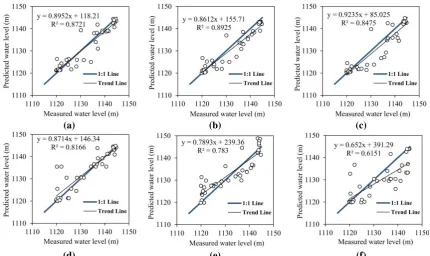
(d) (e) (f)

Figure 6. Results obtained from data-driven models in test stage for simulating piezometer 20 level variations; (a) ANN-PSO, (b) ANN-LM, (c) ANN-HS, (d) RDT, (e) MLR, (f) CDT

(a) (b) (c)

(d) (e) (f)

(a) (b) (c)

(d) (e) (f)

Figure 8. Results obtained from data-driven models in test stage for simulating piezometer 30 level variations; (a) MLR, (b) ANN-HS, (c) ANN-PSO, (d) RDT, (e) ANN-LM, (f) CDT

For piezometer 20, the best performance was obtained by combination ANN-PSO algorithm (considering RMSE criterion), while piezometer 28 exhibited its best performance in combination of ANN-HS algorithm. Besides, piezometer 30 showed its best performance by applying MLR method.

The Man-Whitney test can be used to investigate two groups' dependence or independence from the observed data. The initial hypothesis (H0) is that the two groups of data are equal, and the hypothesis-1 is that the average of the two groups of data are not statistically equal at a certain confidence level. The correct hypothesis can be determined by calculating the p-value at the given confidence level (α); so that, if the p-value is smaller than α, the H0 (equality of the two groups) will be rejected, and otherwise it will be accepted. In the present study, in order to answer the question that whether or not different soft computing methods used in the study have statistically significant differences, it was attempted to statistically investigate the case and perform the Man-Whitney test, the results of which are provided in Table (7).

Table 7- Statistical investigation of results obtained via Man-Whitney method

Piezometer Model p-value Significantly different

(95%)

Significantly different (99%)

20

Observed vs. ANN-LM 0.142 NO NO

Observed vs. ANN-HS 0.156 NO NO

Observed vs. ANN-PSO 0.872 NO NO

Observed vs. CDT 0.136 NO NO

Observed vs. RDT 0.979 NO NO

Observed vs. MLR 0.433 NO NO

28

Observed vs. ANN-LM 0.483 NO NO

Observed vs. ANN-HS 0.921 NO NO

Observed vs. ANN-PSO 0.491 NO NO

Observed vs. CDT 0.135 NO NO

Observed vs. RDT 0.815 NO NO

Observed vs. MLR 0.659 NO NO

30

Observed vs. ANN-LM 0.123 NO NO

Observed vs. ANN-HS 0.736 NO NO

Observed vs. ANN-PSO 0.533 NO NO

Observed vs. CDT 0.106 NO NO

Observed vs. RDT 0.921 NO NO

Observed vs. MLR 0.831 NO NO

In Table (7), the results of the data driven models obtained by various methods were evaluated using Man-Whitney test. The results in Table (7) indicate that in all the models used in this study there was no significant difference between the modelling methods.

In this study, the hydraulics of governing equations for modelling the piezometric are actually captured by the black-box nature of the ANN models by adjusting synaptic weights in their structure. It is highly recommended to compare the results of numerical/mathematical methods for predicting the piezometric with the soft computing models. However, due to the limitation of having precise databases (such as hydraulic conductivity coefficient in the body of dam/foundation) for setting up numerical/mathematical, this could not be achieved in this study.

4. Conclusion

Soft computing is of special importance for solving the nonlinear problems. In this regard, the ANNs as well as their combination with meta-heuristic algorithms are highly regarded in solving the engineering problems. These networks are indeed powerful tools for optimizing the learning and generalizing the training samples; besides, they are among the most important soft computing sub-branches of the decision trees, which are commonly capable to predict and classify the quantitative and qualitative data and are widely used for solving the hydraulic and non-hydraulic problems.

relevant problems; therefore, dam seepage monitoring and also dam surveillance are of special importance for the safety of the dam. On this basis, the present study attempted to investigate the prediction of water level of piezometers of double-curvature arch dam using feed-forward multi-layer artificial neural network (FNN) with Levenberg-Marquardt optimization algorithm as well as PSO and HS algorithms along with classification and regression decision trees and multivariate linear regression model. Despite the appropriate performance of the methods used in simulating the piezometric water level variations, analysis of the statistical results of the used methods revealed the superiority of none of the method over the other ones.

References

1. Rankovic, V. Novakovic, A. Grujovic, N. Divac, D. & Milivojevic, N. 2014

Predicting piezometric water level in dam via artificial neural network. Neural Computing & Applications 24 (5), 1115-1121.

2. Li, M. C. Guo, X. Y. Shi, J. & Zhu, Z. B. 2015 Seepage and stress of anti- seepage structures constructed with different concrete materials in an RCC gravity dam.Water Science and Engineering 8 (4), 326-334.

3. Tan, X. Wang, X. Khoshnevisan, S. & Hou, X. 2017 Seepage analysis of earth dams considering spatial variability of hydraulic parameters. Engineering Geology 228, 260-269.

4. Xiang, Y. Fu, Y. S. Zhu, K. Yuan, H. & Fang, Z. Y. 2017 Seepage safety monitoring model of an earth rock dam under influence of high-impact typhoons on particle swarm optimization method. Water science and Engineering 10 (1), 70-77.

5. Zhou, C. B. Liu, W. Chen, Y. F. Hu, R. & Wei. K. 2015 Inverse modeling of leakage through a rockfill dam foundaction during its construction stage using transient flow model, neural network and genetic algorithm. Engineering Geology 187, 183-195.

6. Su, H. Tian, S. Kang, Y. Xie, W. & Chen, J.2017 Monitoring water seepage velocity in dikes using distributed optical fiber temperature sensors. Automation in Construction 76, 71-84.

7. Turkmen, S. Ozguler, E. Taga, H. & Karaogullarindan, T. 2002 Seepage problems in the karstic limestone foundation of the Kalecik Dam (south Turkey). Engineering Geology 63 (3-4), 247-257.

8. Tayfur, G. Swiatek, D. Wita, A. & Singh, V.P. 2005 Case study: finite element method and artificial neural network models for flow through Jeziorsko Earthfill Dam in Poland. Journal of Hydraulic Engineering 131 (6), 431-440.

10. Stojanovic, B. Milivojevic, M. Milivojevic, N. & Antonijevic, D. 2016 A self-tuning system for dam behavior modeling based on evolving artificial neural network. Advances in Engineering Software 97, 85-95.

11. Nourani, V. Mousavi, S. Sadikoglu, F. & Singh, V. 2017 Experimental and AI-based numerical modeling of contaminant transport in porous media.Journal of Hydrology 205, 78-95.

12. Peymab Company. 1991 Report of Jiroft Dam Study.

13. Zounemat-Kermani, M., 2012 Hourly predictive Levenberg–Marquardt ANN and multi linear regression models for predicting of dew point temperature. Meteorology and Atmospheric Physics, 117(3-4),181-192.

14. Breiman, L. Friedman, J. H. Olshen, R. A. & Stone, C.J. 1984 Classification and regression tree. Chapman & Hall/CRC.

15. Swetapadma, A., & Yadav, A. (2017). A novel decision tree regression-based fault distance estimation scheme for transmission lines. IEEE Transactions on Power Delivery, 32(1), 234-245.

16. Lagacherie, P. & Holmes, S. 1997 Addressing geographical data errors in a classification tree for soil unit prediction. International Journal Geographical Information Science 11 (2),183-198.

17. Salazar, F. Toledo, M. A. Onate, E. & Suarez, B.2016 Interpretation of dam deformation and leakage with boosted regression tree. Engineering Structures 119, 230-251.

18. Nerini, D. Durbec, J. P. Mante, C. Garcia, F. & Ghattas, B. 2000 Forecasting physicochemical variables by a classification tree method application to the Berre Lagoon (South France). Acta Biotheoretica 48 (3-4), 181-196.

19. Paensuwan, N. Yokoyma, A. Verma, S.C. & Nakachi, Y. 2011 Application of Decision Tree Classification to the Probabilistic TTC Evaluation. Journal of International Council on Electrical Engineering 1 (3), 223-330

20. Seyedashraf, O. Rezaei, A. & Akhtari, A. A. 2017 Dam break flow solution using artificial neural network. Ocean Engineerig 142, 125-132.

21. Zounemat-Kermani, M., 2014 Principal component analysis (PCA) for estimating chlorophyll concentration using forward and generalized regression neural networks. Applied Artificial Intelligence, 28(1), pp.16-29.

23. Alsmadi, M. K. S. Omar, K. B. & Noah, S.A. 2009 Back Propagation Algorithm: The Best Algorithm among Multi-layer Perceptron Algorithm. International Journal of Computer Science and Network Security. 9,378-383.

24. Hamid, N. A. Nawi, N. M. GhaZali, R. & Salleh, M. N. M . 2011 Accelerating Learning Performance of Back Propagation Algorithm by Using Adaptive Gain Together with Adaptive Momentum and Adaptive Learning Rate on Classification Problems. International Journal of Software Engineering and its Applications 5, 31-44.

25. Zounemat-Kermani, M., Kisi, O. and Rajaee, T., 2013. Performance of radial basis and LM-feed forward artificial neural networks for predicting daily watershed runoff. Applied Soft Computing, 13(12), pp.4633-4644.

26. Kennedy, J. Eberhart, R. 1995 Particle swarm optimization. In: Proceedings of the 1995 IEEE I nternational Conference on Neural Networks, Perth, 4, 1942-1948.

27. Chau, K.W. 2006 Particle swarm optimization training algorighm for ANNs in stage prediction of Shing Mun River. Journal of Hydrology 329 (3-4), 363-367.

28. Gyanesh, D. Prasant, K. P. & Sasmita, K. P. 2014 Artificial Neural Network trained by particle swarm optimization for non-linear channel equalization. Expert Systems with Application 41 (7), 3491-3496.

29. Xiang, Y. Fu, Y. S. Zhu, K. Yuan, H. & Fang, Z. Y. 2017 Seepage safety monitoring model of an earth rock dam under influence of high-impact typhoons on particle swarm optimization method. Water science and Engineering 10 (1), 70-77.

30. Mun, S. & Cho, Y. H. 2012 Modified harmony search optimization for constrained design problems. Expert Systems Applications 39 (1), 419-423.

31. Geem, Z. W. Kim, J. & Loganathan, G. 2002 Harmony search optimization: Application to pipe network design. International Journal of Model Simulation 22, 125-133.

32. Yadav, P. Kumar, R. Panda, S. K. Chang, C.S. 2012 An Intelligent Tuned Harmony Search algorithm for optimization. Information science 196, 47-72.

33. Ruby, M. & Botez, R. M. 2016 Trajectory Optimization for vertical navigation using the Harmony Search algorithm. IFAC-PapersOnLine 49 (17), 11-16.