Lattice Boltzmann Methods for Fluid Structure Interaction

(1)

Calhoun: The NPS Institutional Archive

Theses and Dissertations Thesis Collection

2012-09

Lattice Boltzmann Methods for Fluid Structure Interaction

Blair, Stuart R.

Monterey, California. Naval Postgraduate School

(2)

MONTEREY, CALIFORNIA

DISSERTATION

LATTICE BOLTZMANN METHODS FOR FLUID STRUCTURE INTERACTION

by Stuart R. Blair September 2012

Dissertation Supervisor: Young Kwon

(3)

(4)

REPORT DOCUMENTATION PAGE Form Approved OMB No. 0704-0188

Public reporting burden for this collection of information is estimated to average 1 hour per response, including the time for reviewing instruction, searching existing data sources, gathering and maintaining the data needed, and completing and reviewing the collection of information. Send comments regarding this burden estimate or any other aspect of this collection of information, including suggestions for reducing this burden, to Washington headquarters Services, Directorate for Information Operations and Reports, 1215 Jefferson Davis Highway, Suite 1204, Arlington, VA 22202-4302, and to the Office of Management and Budget, Paperwork Reduction Project (0704-0188) Washington DC 20503.

1. AGENCY USE ONLY (Leave blank) 2. REPORT DATE

September 2012

3. REPORT TYPE AND DATES COVERED

Dissertation

4. TITLE AND SUBTITLE: Lattice Boltzmann Methods for Fluid Struc-ture Interaction

5. FUNDING NUMBERS

6. AUTHOR(S): Stuart R. Blair

7. PERFORMING ORGANIZATION NAME(S) AND ADDRESS(ES) 8. PERFORMING ORGANIZATION REPORT NUMBER

9. SPONSORING/MONITORING AGENCY NAME(S) AND ADDRESS(ES) 10. SPONSORING/MONITORING AGENCY REPORT NUMBER

11. SUPPLEMENTARY NOTES: The views expressed in this thesis are those of the author and do not reflect the official policy or position of the Department of Defense or the U.S. Government. IRB Protocol Number: NA.

12a. DISTRIBUTION / AVAILABILITY STATEMENT

Approved for public release; distribution is unlimited

12b. DISTRIBUTION CODE

A

13. ABSTRACT (maximum 200 words)

The use of lattice Boltzmann methods (LBM) for fluid flow and its coupling with finite element method (FEM) structural models for fluid-structure interaction (FSI) is investigated. A body of high performance LBM software that exploits graphic processing unit (GPU) and multiprocessor programming models is developed and validated against a set of two- and three-dimensional benchmark problems. Computational performance is shown to exceed recently reported results for single-workstation implementations over a range of problem sizes. A mixed-precision LBM collision algorithm is presented that retains the accuracy of double-precision calculations with less computational cost than a full double-precision implementation. FSI modelling methodology and example applications are presented along with a novel heterogeneous parallel implementation that exploits task-level parallelism and workload sharing between the central processing unit (CPU) and GPU that allows significant speedup over other methods. Multi-component LBM fluid models are explicated and simple immiscible multi-Multi-component fluid flows in two-dimensions are presented. These multi-component fluid LBM models are also paired with structural dynamics solvers for two-dimensional FSI simulations. To enhance modeling capability for domains with complex surfaces, a novel coupling method is introduced that allows use of both classical LBM (CLBM) and a finite element LBM (FELBM) to be combined into a hybrid LBM that exploits the flexibility of FELBM while retaining the efficiency of CLBM.

14. SUBJECT TERMS

lattice Boltzmann method, fluid-structure interaction

15. NUMBER OF PAGES 161 16. PRICE CODE 17. SECURITY CLASSIFICATION OF REPORT Unclassified 18. SECURITY CLASSIFICATION OF THIS PAGE Unclassified 19. SECURITY CLASSIFICATION OF ABSTRACT Unclassified 20. LIMITATION OF ABSTRACT UU

NSN 7540-01-280-5500 Standard Form 298 (Rev. 2-89)

(5)

(6)

Approved for public release; distribution is unlimited

LATTICE BOLTZMANN METHODS FOR FLUID STRUCTURE INTERACTION

Stuart R. Blair

Commander, United States Navy B.S., United States Naval Academy, 1994 M.S., Massachusetts Institute of Technology, 2003 Nuclear Eng., Massachusetts Institute of Technology, 2003

Submitted in partial fulfillment of the requirements for the degree of

DOCTOR OF PHILOSOPHY IN MECHANICAL ENGINEERING

from the

NAVAL POSTGRADUATE SCHOOL September 2012 Author: Stuart R. Blair Approved By: Young W. Kwon Distinguished Professor

Dept. of Mech. & Aero. Engineering Dissertation Committee Chair

Garth V. Hobson Professor

Dept. of Mech. & Aero. Engineering

Joshua H. Gordis Associate Professor

Dept. of Mech. & Aero. Engineering

Clyde L. Scandrett Professor

Dept. of Applied Mathematics

Francis X. Giraldo Professor

Dept. of Applied Mathematics Approved By:

Knox T. Millsaps, Professor & Chair, Dept. of Mechanical & Aerospace Engineering Approved By:

(7)

(8)

ABSTRACT

The use of lattice Boltzmann methods (LBM) for fluid flow and its coupling with finite el-ement method (FEM) structural models for fluid-structure interaction (FSI) is investigated. A body of high performance LBM software that exploits graphic processing unit (GPU) and multiprocessor programming models is developed and validated against a set of two- and three-dimensional benchmark problems. Computational performance is shown to exceed recently reported results for single-workstation implementations over a range of problem sizes. A mixed-precision LBM collision algorithm is presented that retains the accuracy of double-precision calculations with less computational cost than a full double-precision im-plementation. FSI modelling methodology and example applications are presented along with a novel heterogeneous parallel implementation that exploits task-level parallelism and workload sharing between the central processing unit (CPU) and GPU that allows signifi-cant speedup over other methods. Multi-component LBM fluid models are explicated and simple immiscible multi-component fluid flows in two-dimensions are presented. These multi-component fluid LBM models are also paired with structural dynamics solvers for two-dimensional FSI simulations. To enhance modeling capability for domains with com-plex surfaces, a novel coupling method is introduced that allows use of both classical LBM (CLBM) and a finite element LBM (FELBM) to be combined into a hybrid LBM that exploits the flexibility of FELBM while retaining the efficiency of CLBM.

(9)

(10)

LIST OF FIGURES

Figure 1. The D2Q9 lattice. . . 7

Figure 2. Commonly used lattice topologies for LBM in three dimensions. . . . 8

Figure 3. Schematic of lattice point on west domain boundary. . . 15

Figure 4. Streaming off2 across a North/South periodic boundary. . . 15

Figure 5. Application of on-grid bounce-back boundary condition. . . 16

Figure 6. Half-way bounceback solid boundary condition schematic. . . 17

Figure 7. Groups of density distributions on west boundary lattice point. . . 19

Figure 8. Scaling from physical units, to dimensionless units to LBM units. . . 24

Figure 9. Schematic diagram of channel flow example problem. . . 25

Figure 10. LBM time step flowchart. . . 29

Figure 11. Velocity magnitude, pressure, and vorticity magnitude for example flow case after 50,000 time steps. . . 30

Figure 12. Poiseuille flow configuration. . . 32

Figure 13. Poiseuille flow convergence with On-Grid bounce-back boundary con-ditions. . . 34

Figure 14. Poiseuille flow convergence with half-way bounce-back boundary con-ditions in single precision. . . 35

Figure 15. Poiseuille flow convergence with half-way bounce-back boundary con-ditions in double precision. . . 35

Figure 16. Poiseuille flow convergence with half-way bounce-back boundary con-ditions using mixed-precision arithmetic. . . 36

Figure 17. Relative performance of single precision (SP), mixed precision (MP) and double precision (DP) computational routines for Poiseuille flow. The lattice refinement parameter refers to the number of lattice points placed across in the dimension of the channel opening. . . 37

Figure 18. Stabilization time for Poiseuille flow, Re=10, _τ1 = ω = 1.3. Top figure, Ny=30, bottom figure, Ny=480. . . 38

Figure 19. Backward step flow separation behavior. Image taken from [34] . . . 40

Figure 20. Schematic of domain and boundary conditions for Backward-Step benchmark in 2D. . . 40

Figure 21. Backward-Step simulation. Step height = 0.25m, outlet width=0.5m, Re=100. . . 41

Figure 22. Comparison of primary vortex re-attachment length normalized by step height with results reported in [35]. . . 41

(15)

Figure 23. Schematic of the two-dimensional lid-driven cavity problem. . . 42

Figure 24. Lid-driven cavity in two dimensions with 1600x1600 lattice showing

from left-to-right streamlines, vorticity contours and pressure con-tours for Re=1000. Top set of figures is LBM from this work. Bottom set of figures is from [36]. . . 43

Figure 25. Lid-driven cavity in two dimensions with 1600x1600 lattice showing

from left-to-right streamlines, vorticity contours and pressure con-tours for Re=5000. Top set of figures is LBM, bottom set of figures is from [37]. . . 43

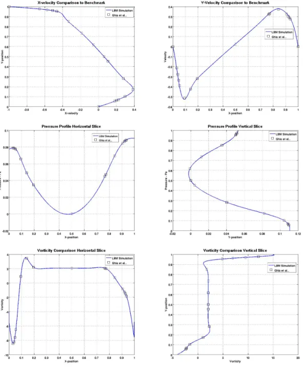
Figure 26. Comparison of velocity, pressure and vorticity to benchmark values

for Re=1000. . . 45

Figure 27. Channel with cylindrical obstacle 2D problem. . . 46

Figure 28. Streamline visualization of trailing vortex at Re=20 (top) and Re=40

(bottom). . . 47

Figure 29. Vorticity plot for cylinder in 2D flow at Re=100. . . 48

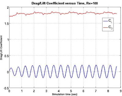
Figure 30. Drag and lift coefficient for cylinder in uniform flow. Re=100. . . 49

Figure 31. Strouhal number computed from the energy spectra of the lift

coeffi-cient at Re=100. . . 49

Figure 32. Historical trends for CPU and GPU memory bandwidth and compute

performance (From [52]). . . 52

Figure 33. Memory bandwidth requirement versus desired computational

through-put for a typical LBM implementation. Modern CPU and GPU hard-ware are memory bandwidth limited for LBM. . . 53

Figure 34. Simplified schematic of NVIDIA GPU. . . 54

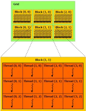
Figure 35. Hierarchy of threads in a CUDA program. Threads are organized into

blocks; blocks are organized into a grid (From [52]). . . 55

Figure 36. Schematic of data layout schemes. (a) depicts the array of structures

(AoS), (b) depicts the structure of arrays (SoA). Superscripts indicate lattice node number, subscripts indicate the lattice velocity. . . 61

Figure 37. When using SoA, load instructions executed by consecutive threads

read from consecutive locations in memory . . . 61

Figure 38. Schematic of the dual lattice scheme used to support a unified time

step kernel. On even time steps, the Even Lattice is active and it

collides and streams to the Odd Lattice; vice versa for odd time steps. 63

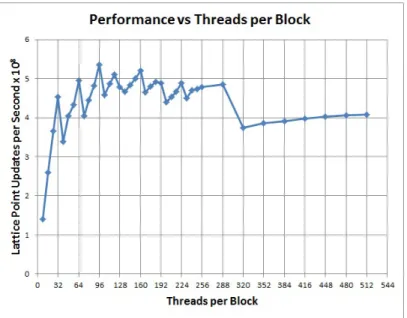
Figure 39. LBM performance on GTX-580 for three-dimension lid-driven cavity

as a function of threads per block. . . 65

Figure 40. Performance benchmark for lattice Boltzmann method (LBM) on a

(16)

Figure 41. LBM on a 3D lid-driven cavity with various number of threads per

block. . . 69

Figure 42. Lid-driven cavity using a D3Q15 lattice with5003_{points using CUDA} and OpenMP. . . 71

Figure 43. Schematic LBM time step for distributed computing with MPI. Scal-ability is achieved by interleaving communication with computation. . 72

Figure 44. Weak scaling using MPI for LBM simulation of three-dimensional Poiseuille flow. . . 73

Figure 45. Weak scaling using CUDA and MPI for LBM simulation of three-dimensional Poiseuille flow. . . 74

Figure 46. Euler-Bernoulli Beam. . . 80

Figure 47. Schematic of 2D converging and diverging duct. . . 82

Figure 48. Converging and diverging duct displacement, velocity and accelera-tion at beam midpoint. Re = 5, glycerin with cork beam. . . 83

Figure 49. Converging and diverging duct with combined beam response. Re=5, glycerin with cork beam. . . 84

Figure 50. Converging and diverging duct with varying fluid viscosity. Starting from top left, fluid viscosity is νglycerin 4 , νglycerin 2 andνglycerin . . . 85

Figure 51. Converging and diverging duct with varying beam elastic modulus. From left to right elastic modulus is Ecork 2 andEcork. . . 85

Figure 52. Schematic diagram of lid-driven cavity FSI problem geometry. . . 86

Figure 53. Results for two-dimensional lid-driven cavity. . . 87

Figure 54. Final bottom displacement. . . 88

Figure 55. Cylinder with elastic fin benchmark . . . 88

Figure 56. Results for two-dimensional cylinder with elastic trailing fin at Re=200. 89 Figure 57. Displacement, velocity and acceleration for cylinder with elastic fin. Re=200. . . 91

Figure 58. Illustration of task-level decomposition in parallel implementation of FSI problem. In the lower figure, a further level of task-level paral-lelism is exploited by overlapping the structural dynamics computa-tion on the CPU with LBM calculacomputa-tions on domain areas remote from the elastic structure on the GPU. . . 92

Figure 59. Decomposition of FSI problem domain for task-level heterogeneous parallelism. . . 93

Figure 60. Schematic of Hybrid LBM time step. Methodology differs only in implementation of the particle streaming phase. . . 99

(17)

Figure 61. Schematic Hybrid Lattice on regular domain. Assignment follow-ing streamfollow-ing in the CLBM domain and advection in the FELBM domain is only made to the interior of each respective sub-domain. Data drawn from the lattice points on the halo facilitates communica-tion between each sub-domain. . . 99

Figure 62. Interface region for CLBM and FELBM domains on a uniform mesh.

Lattice points with both the asterisk and circle belong to the interface. 100

Figure 63. Mid-channel normalized velocity profile for Poiseuille flow using CLBM,

FELBM and HLBM. . . 102

Figure 64. Hybrid lattice mesh around a circular obstacle. Lattice points with

as-terisk are in the CLBM sub-domain, those circled are in the FELBM sub-domain. Those with both markings are members of the interface halo of the two regions. . . 103

Figure 65. Normalized velocity contour plot for fluid flow around circular

obsta-cle at Reynolds number = 5 using CLBM . . . 104

Figure 66. Normalized velocity contour plot for fluid flow around circular

obsta-cle at Reynolds number = 5 using Hybrid LBM. . . 105

Figure 67. Normalized velocity profile at 30 percent channel length, Reynolds

number = 5. . . 106

Figure 68. Normalized velocity profile at 60 percent channel length, Reynolds

number = 5. . . 107

Figure 69. Schematic Hybrid Lattice on regular domain. Assignment

follow-ing streamfollow-ing in the CLBM domain and advection in the FELBM domain is only made to the interior of each respective sub-domain. Data drawn from the lattice points on the halo facilitates communica-tion between each sub-domain. . . 108

Figure 70. Illustration of inter-particle forces in the nearest neighborhood of a

lattice point. . . 112

Figure 71. Two immiscible components. G = -1.2 . . . 115

Figure 72. Two immiscible components. G = -0.2. Note that the weak interaction

parameter renders the fluids miscible. . . 116

Figure 73. Density for Fluid 1 of a two-component immiscible fluid flow in a

lid-driven cavity. Initial configuration. . . 117

Figure 74. Fluid 1 results for a two-component immiscible fluid flow in a

lid-driven cavity. Sequence of images shows flow progression from top to bottom corresponding respectively to early in the simulation to its final steady state. . . 118

(18)

Figure 75. Fluid 1 results for a two-component immiscible fluid flow in a lid driven cavity. The higher viscosity and density of fluid 2 results in its confinement in the bottom-half of the cavity domain. . . 119

Figure 76. Fluid 1 results for a two-component immiscible fluid flow in a lid

driven cavity. The higher viscosity and density of fluid 2 results in its confinement in the bottom-half of the cavity domain. . . 119

Figure 77. Schematic representation of a lid-driven cavity with an elastic beam

attached to the lower surface. . . 120

Figure 78. Single-component fluid flow in cavity with beam. Streamlines show

development of three distinct vortex regions. . . 121

Figure 79. Momentum and density fields for fluid 1 at steady-state; Re=1000. . . 122

Figure 80. Plot of displacement, velocity and acceleration at the tip of the elastic

beam. . . 122

Figure 81. Final beam displacement for multi-component FSI. Beam

(19)

(20)

LIST OF TABLES

Table 1. Geometry and fluid parameters for Poiseuille flow test case. . . 32

Table 2. Comparison of trailing vortex length to benchmark values. . . 46

Table 3. Comparison of Strouhal number to benchmark values. . . 48

Table 4. Memory bandwidth of various CUDA memory spaces on an NVIDIA

GTX-580 GPU . . . 64

Table 5. Properties of GPU devices used in benchmark computations in Figure

40 . . . 67

Table 6. Selected structural material properties used for fluid-structure interaction

(FSI) simulations. . . 81

Table 7. Selected fluid properties for FSI simulations. . . 81

Table 8. Performance improvement from using overlapped execution depicted

in lower half of Figure 58 versus the non-overlapped scheme in the top half of Figure 58. The lattice was 22 x 337 x 526 D3Q19 using MRT collision operator. The structural model was a sheer-deformable plate with 2883 degrees of freedom. . . 94

(21)

(22)

LIST OF ACRONYMS AND NOMENCLATURE

API application programming interface

AoS array of structures

BGK Bhatnagar-Gross-Krook

CLBM classical lattice Boltzmann method

CUDA Compute Unified Device Architecture

DEM discrete element method

LBM lattice Boltzmann method

FELBM finite element lattice Boltzmann method

FEM finite element method

FSI fluid-structure interaction

FVM finite volume method

GB gigabytes

GFLOPS billion floating point operations per second

GPU graphical processing unit

HLBM hybrid lattice Boltzmann method

IB immersed boundary

LBGK lattice Bhatnagar-Gross-Krook

MPI message passing interface

MRT multiple relaxation time

SM Streaming Multiprocessor

SP Scalar Processors

SoA structure of arrays

(23)

cs lattice Boltzmann method lattice sound speed

eα lattice velocity

fα particle density distribution function

feq

α equilibrium density distribution function

M particle moment transformation operator

ν kinematic viscosity

Ωα collision operator

p macroscopic pressure

ρ macroscopic density

R particle moment space

S multiple relaxation time relaxation matrix

τ relaxation time

u macroscopic velocity

ω single relaxation-time relaxation operator

(24)

I. INTRODUCTION

The present thesis investigates the use of the lattice Boltzmann method (LBM) to solve for the flow of viscous, incompressible fluids while accounting for the effect these fluid flows have on surrounding elastic structures. From waves slapping against ship struc-tural members, cooling water passing over heat-exchanger tubes to blood flowing within veins and arteries among many others, FSI has applications that span the engineering and life sciences. Towards the goal of simulating such physical behavior, several intermediate steps were required. These intermediate steps start with the development of a robust and highly capable software tool for simulating and analyzing flow of incompressible viscous fluids and continue through to integration of these tools with structural dynamics solvers.

A. OBJECTIVES AND ORGANIZATION

The first objective is to develop software tools required for a LBM flow solver that can reliably and accurately simulate fluid flow problems of interest. The theory and formulation of the LBM, including detailed considerations of stability, accuracy and proper scaling of simulation variables to allow modeling of specific fluid systems is provided in Chapter II.

With a detailed understanding of the theory, software tools can be developed to simulate fluid flows of interest. Such software is developed and subjected to a collection of validation benchmarks in Chapter III. The second-order convergence of the LBM along with select boundary conditions is demonstrated along with a demonstration of the potential impacts of the wide use of single-precision arithmetic on this convergence rate. A mixed-precision LBM implementation is introduced that provides for second-order convergence for select boundary conditions while retaining some of the performance benefits of using single precision number representation and arithmetic.

(25)

In order to increase the accuracy of a LBM simulation, the spatial and temporal dis-cretization is refined. Smaller time steps and a more refined lattice both lead to increased computational demand. In order to execute LBM simulations in a reasonable amount of time, the programs are written to be executed in parallel. In Chapter IV the Compute Uni-fied Device Architecture (CUDA) programming model is introduced and the implementa-tion of the LBM programs for parallel execuimplementa-tion on a graphical processing unit (GPU) is described. The achieved performance is compared with recently published benchmarks. Two hybrid programming models are also demonstrated that use a combination of CUDA and OpenMP in one case and CUDA and message passing interface (MPI) in another. Collectively, Chapter IV describes the development of a scalable high-performance LBM solver.

Once reliable fluid simulation tools are in place, the second objective is to couple this fluid solver with an appropriate structural dynamics model. These software compo-nents are then used as coupled FSI simulation tools. The key ingredients of computing forces and moments along the fluid-structure interface and accounting for their exchange and integrating with a structural dynamics solver for a coordinated FSI simulation are dis-cussed. The specific methods and algorithms for doing this along with example applications in both two and three dimensions are presented in Chapter V.

The aforementioned software tools were all developed based on the classical LBM theory. A recently developed modification, termed the finite element lattice Boltzmann method (FELBM), allows use of unstructured non-uniform finite element grids in lieu of the regular structured grid from classical lattice Boltzmann method (CLBM). The FELBM gains this flexibility at the expense of some computational efficiency on a per-lattice-point basis. An algorithm and associated software tool has been developed resulting in a hybrid lattice Boltzmann method (HLBM) whereby both CLBM and FELBM are used on disjoint sub-domains of an overall simulation. This hybrid tool leverages the simplicity and effi-ciency of the CLBM while also benefiting from the geometric flexibility of the FELBM. The overall system is able to simulate fluid flow over the combined domain with less

(26)

com-putational effort than the FELBM while reducing the memory requirements of an equiv-alent simulation using only CLBM. The theory and algorithms for accomplishing this is provided in Chapter VI.

The last objective of this model is to take advantage of the flexible and physically intuitive methods for modeling multi-component fluid systems using LBM. A discussion of the standard LBM theory for multi-component fluids as well as example problems in fluid flow and FSI are demonstrated in Chapter VII.

In Chapter VIII, conclusions and prospects for future research are discussed.

B. STATEMENT OF CONTRIBUTIONS

The principal contributions of this thesis are:

• A body of software tools that provide LBM modeling capability for

single-component incompressible viscous flows in two and three dimensions.

• A new mixed-precision LBM implementation that retains most of the

ac-curacy of double precision while requiring only the memory of single pre-cision.

• A GPU-accelerated implementation of LBM with highly competitive

per-formance against recently published benchmarks.

• A new method to simulate two-way FSI that exploits task-level

concur-rency for a heterogeneous-parallel algorithm using both GPU for the fluid domain and central processing units for the solid domain.

• A novel method for combining CLBM and FELBM into a HLBM.

• LBM flow and FSI modeling capability for multi-component flows in two

(27)

(28)

II. LATTICE BOLTZMANN METHOD

The LBM is an increasingly popular way to simulate fluid flow. In contrast to more conventional methods such as finite difference methods (FDM) control volume meth-ods (CVM) and finite element methmeth-ods (FEM), the LBM begins not with the picture of the fluid as a continuous medium, but instead as a collection of particles. These parti-cles move and undergo local interactions with other partiparti-cles in accordance with simple rules. Macroscopic physical phenomena such as those conservation laws described by the Navier-Stokes equations emerge from the large number of these local interactions. The microscopic level of description provides an intuitive basis for generalization to complex systems such as porous media ([1]-[3]), two-phase flow ([4]-[6]) and magnetohydrodynam-ics ([7]-[9]) among others. By judiciously altering the formulation, other partial differen-tial equations of interest have been modeled by a similar procedure including the Burgers Equation [10], the Korteweg-de Vries equation [11], the Brinkman equation [12] and the Schr¨odinger equation [13]. For a concise review of the current state of the art in LBM, an excellent survey can be found in [14] with a recent update in [15]. A recently published analysis of LBM theory, which includes a thorough critique and comparison with tradi-tional computatradi-tional fluid dynamics techniques, can be found at [16]. In this work, the LBM will be used for the solution of the Navier-Stokes equations for single-component fluid flows as well as a limited number of multi-component fluid flows.

This chapter will start with a brief overview of the historical development of the LBM. This will be followed by a description of each element of a LBM simulation in-cluding typical lattice structures with lattice velocities and associated weights, collision operators, boundary conditions, body forces and scaling requirements. The chapter will be concluded with a detailed example application of the LBM to two-dimensional channel flow over a cylindrical obstacle.

(29)

A. LITERATURE REVIEW AND INTRODUCTION

Historically, the LBM is derived from the concepts of the cellular automaton [17], [18]. Space is described by a regular array of interconnecting lattice sites and time is di-vided into equally spaced time-steps. The cellular automata model is specified by stating the rules by which each lattice site shall be updated for the next time step. Depending on these rules, complex physical phenomena emerge [19]. A classical example of complex be-havior emerging from simple rules is Conway’s Game of Life. In some cases, the CA with associated sets of update rules have become useful as a model for real physical behavior and have become a means to gaining more fundamental understanding. Examples include traffic flow [20], population dynamics [21], and earthquake prediction [22] to name but a few.

The CA model underlying a fluid dynamics model incorporates movement of par-ticles from one lattice site to another along discrete lattice directions. The rule for lattice site update is applied to all particles arriving at a given lattice site in a given time step and is represented formally in Equation 1,

Nα(x+δxeα, t+δt) =Nα(x, t) + Ωα(N) (1)

whereNα is a Boolean variable indicating the presence or absence of a fluid particle

trav-eling along lattice direction eα at position x. The rules for update—referred to as the

Collision Operator—are formally denoted byΩα(N). One advantage of this formulation

using Boolean variables is the absence of round-off errors; all arithmetic is exact. Unfor-tunately, though the mathematical operations are simple and exact, it has been found that they are required in enormous numbers to overcome statistical noise in the results. Ad-ditionally, it has been found that further lattice symmetry requirements need to be met in order to provide Galilean invariance.

The LBM emerged from the solutions presented to these difficulties [18], [23]. The LBM seeks to solve the discrete Boltzmann equation which, in the absence of external

(30)

forces is:

∂fα

∂t +eα· ∇fα = Ωα , α∈[0, . . . , q] ,eα ∈R

d ₍₂₎

wherefαis the particle velocity distribution function for lattice directionα;eα is the set of

lattice velocities; andΩαis the collision operator. Additionally, initial values for allfαmust

be supplied on the problem domain and boundary conditions must be applied appropriately. In the following sections, each of these issues will be addressed in turn so that a simulation of fluid flow may be undertaken using the LBM.

B. LATTICE STRUCTURES

In the LBM, this solution is sought on a regular lattice. A lattice is defined by a

sound speedcs, a set ofd-dimensional lattice velocitieseα whereα ∈ [0, . . . , q]and a set

of weightswα. The usual notation to specify a lattice is given as DdQq. A lattice commonly

used in two dimensions has nine velocities and is denoted D2Q9 and is illustrated in Figure 1. The sound speed, weights and lattice velocities for this model are given in Equation 3.

(31)

c2_s = 1₃ w0 = 2₉ w1−4 = 1₉ w5−8 = ₃₆1 e0 = (0,0) e1 = (1,0) e2 = (0,1) e3 = (−1,0) e4 = (0,−1) e5 = (1,1) e6 = (−1,1) e7 = (−1,−1) e8 = (1,−1) (3)

Commonly used lattices for three-dimensional problems are shown in Figure 2. Sets

of lattice speeds are given for theD3Q15lattice are given in Equation 4, and those for the

D3Q19andD3Q27are shown respectively in Equations 5 and 6.

Figure 2: Commonly used lattice topologies for LBM in three dimensions.

c2_s = 1₃ w0 = 2₉ w1−6 = 1₉ w7−14= ₇₂1 e0 = (0,0,0) e1 = (1,0,0) e2 = (−1,0,0) e3 = (0,1,0) e4 = (0,−1,0) e5 = (0,0,1) e6 = (0,0,−1) e7 = (1,1,1) e8 = (−1,1,1) e9 = (1,−1,1) e10 = (−1,−1,1) e11= (1,1,−1) e12= (−1,1,−1) e13 = (1,−1,−1) e14 = (−1,−1,−1) (4)

(32)

c2_s = 1₃ w0 = 1₃ w1−6 = ₁₈1 w7−19 = ₃₆1 e0 = (0,0,0) e1 = (1,0,0) e2 = (−1,0,0) e3 = (0,1,0) e4 = (0,−1,0) e5 = (0,0,1) e6 = (0,0,−1) e7 = (1,1,0) e8 = (−1,1,0) e9 = (1,−1,0) e10 = (−1,−1,0) e11 = (1,0,1) e12= (−1,0,1) e13= (1,0,−1) e14 = (−1,0,−1) e15 = (0,1,1) e16= (0,−1,1) e17= (0,1,−1) e18 = (0,−1,−1) (5) c2 s = 1 3 w0 = ₂₇8 w1−3,14−16 = ₂₇2 w10−13,23−26= ₅₄1 w4−9,17−22 = ₂₁₆1 e0 = (0,0,0) e1 = (−1,0,0) e2 = (0,−1,0) e3 = (0,0,−1) e4 = (−1,−1,0) e5 = (−1,1,0) e6 = (−1,0,−1) e7 = (−1,0,1) e8 = (0,−1,−1) e9 = (0,−1,1) e10 = (−1,−1,−1) e11= (−1,−1,1) e12= (−1,1,−1) e13 = (−1,1,1) e14 = (1,0,0) e15= (0,1,0) e16= (0,0,1) e17 = (1,1,0) e18 = (1,−1,0) e19= (1,0,1) e20= (1,0,−1) e21 = (0,1,1) e22 = (0,1,−1) e23= (1,1,1) e24= (1,1,−1) e25 = (1,−1,1) e26 = (1,−1,−1) (6)

The values of cs, wα and the vectors eα are all selected so as to satisfy a set of

symmetry conditions given in Equation 7.

P αwα = 1 P αwαcαi = 0 P αwαcαicαj =c 2 sδij P_αwαcαicαjcαl= 0 P αwαcαicαjcαkcαlcαm = 0 P αwαcαicαjcαlcαm =c 4 s(δijδlm+δilδjm+δimδjl) (7)

(33)

These symmetry conditions play an important roll in the theory of LBM. In particular, they are needed to show the correspondence between the LBM and the incompressible Navier-Stokes equation. It can be shown that all of the lattices introduced satisfy these conditions. The discrete Boltzmann Equation shown in Equation 2 is in the general form of an

advection equation. The momentum space is discretized along theq lattice speeds which,

with the advection equation analogy, are the characteristic speeds. The right hand side of

Equation 2 is the collision operatorΩαwhich determines what happens to the particle

pop-ulationsfα as they traverse the lattice in their respective characteristic directions. Instead

of numerically integrating the temporal and spatial derivative operators, the LBM handles them discretely in time and space by “streaming” particle distributions from a source lattice site to neighboring lattice site in each direction. This process is illustrated schematically

with the arrows in in Figure 1 and is formally expressed in Equation 8 whereris the

posi-tion vector for a given lattice point andtis the current time in lattice units.

fα(r+eα, t+ 1)−fα(r, t) = Ωα. (8)

The simplest and most popular form for the collision operator is the Bhatnagar-Gross-Krook (BGK), shown in Equation 9, which gives a single-parameter relaxation to equilibrium:

ΩBGK_α =−1

τ (fα−f

eq

α ) (9)

whereτ is a relaxation parameter, f_αeq is a function of the macroscopic parameters of the

fluid represented byfαgiven by Equation 10.

f_αeq =ρwα " 1 + (eα·u) c2 s +(eα·u) 2 c4 s − 1 2 (u·u) c2 s # (10)

(34)

computed as moments of the particle distribution functionfαas shown in Equations 11 and

12. When required for physical modeling, the fluid pressure pcan also be obtained from

Equation 13. ρ= q−1 X α=0 fα (11) u = 1 ρ q−1 X α=0 fαeα (12) p=ρc2_s (13)

The relaxation parameterτ can be related to the fluid kinematic viscosityν. This

relation-ship is given in Equation 14 with all units expressed in lattice units.

τ = ν c2

s

+1

2 (14)

Frequently in the literature, and periodically in this thesis, the inverse ofτ is used

as the relaxation parameter and is conventionally named ω. Since for real fluids, ν must

be non-negative, τ is constrained to be greater than or equal to 1₂. In notation employing

ω, this implies 0 ≤ ω ≤ 2. In a later section of this thesis where dimensional scaling

and stability are discussed, it will be demonstrated that the numerical stability of any given

LBM simulation can be characterized by the value ofτ orω. Systems where the combined

fluid properties, boundary conditions and LBM spatial and temporal discretizations result in

the value ofωto be close to 2, or converselyτ approaching 1₂, tend to become numerically

unstable.

C. MULTIPLE RELAXATION TIME COLLISION OPERATOR

While the single relaxation time lattice Bhatnagar-Gross-Krook (LBGK) operator is easy to implement and computationally efficient within the context of a single LBM time

(35)

step, it is known to suffer from severe stability problems. When these stability problems can be overcome while still using LBGK, it is often only obtained at the expense of an increase in lattice density and hence, increase in computational effort. The LBGK has other deficiencies including an implied fixed Prandtl number of one and a fixed ratio between kinematic and bulk viscosity. In order to provide a means for tuning the stability properties of a given simulation while also a mechanism for altering more specific fluid properties, alternative collision operators have been developed.

The multiple relaxation time (MRT) collision operator, also referred to as the gener-alized lattice Boltzmann equation, was first presented in [24]. Its objectives were to resolve the fixed Prandtl number defect of LBGK, and allow for varying kinematic and bulk vis-cosities as well as introduce a mechanism for increasing simulation stability. The MRT

projects the density distribution functionsfαonto an orthogonal vector space of momenta

of the vector space using the operator M. The particular momenta depend on the lattice

structure chosen but all include a combination of the mass density, kinetic energy,

mo-mentum flux, energy flux and viscous stress tensor. They are expressed in the vectorR.

Relaxation occurs over the momentum space using the relaxation times given inSand the

result is transformed back to the density spacefα using the inverse ofM.

For the D2Q9 lattice, the momentum space and transformation matrix are given in Equations 15 and Equation 16, respectively.

RD2Q9 =

h

ρ e jx qx jy qy pxx qxy

iT

(36)

MD2Q9 =                        1 1 1 1 1 1 1 1 1 −4 −1 −1 −1 −1 2 2 2 2 4 −2 −2 −2 −2 1 1 1 1 0 1 0 −1 0 1 −1 −1 1 0 −2 0 2 0 1 −1 −1 −1 0 0 1 0 −1 1 1 −1 −1 0 0 −2 0 2 1 1 −1 −1 0 1 −1 1 −1 0 0 0 0 0 0 0 0 0 1 −1 1 −1                        (16)

where R = Mfα and ρ is fluid density, e is the energy, is related to the square of the

energy, jx and jy are mass fluxes, qx and qy correspond to energy flux and pxx and pxy

correspond to the diagonal and off-diagonal components of the viscous stress tensor. The coefficients for relaxation over this momentum space are given in a diagonal matrix as in Equation 17.

S =diag(0, s2, s3,0, s5, s7, s8, s9) (17)

In [25] it was shown that the same fluid viscosity is given in the fluid flow whens8 =s9 =

1

τ. The other parameters in Equation 17 can be set as desired so as to promote solution

stability or as required to further tailor fluid behavior. If all non-zero coefficients ofSare

set to 1_τ, LBGK single-relaxation time is recovered. Having specified the coefficients ofS,

the LBM collision operator is as shown in Equation 18,

ΩMRT =−M−1SM(f−feq) (18)

where all values offα are relaxed with a single matrix collision operator. In the software

developed for this work, it has been observed that use of MRT significantly promotes simu-lation stability. While the MRT requires more computations per time-step, it has been found

(37)

that simulations are able to be conducted with much lower lattice density. Furthermore, fewer time steps are typically required for flows to overcome the noise of nonequilibrium initial conditions and reach accurate flow configurations.

D. BOUNDARY CONDITIONS

The fluid flow problems which we hope to solve using LBM are initial boundary value problems. As such, the handling of initial and boundary conditions should be central to any discourse on numerical solution methods.

One problem with LBM is that the physically relevant and observable macroscopic flow features such as velocity and pressure are not the dependent variables in the governing equation; rather they are functions of the dependent variables. While it is possible to find a

reasonable set offα corresponding to a particular pressure and velocity there is in general

no unique way to do this.

Despite this difficulty, researchers have formulated numerous schemes that try to view the boundary lattice points in a manner consistent with every other lattice point with the exception that, for certain lattice directions there is no updated data streamed in from the previous time step. This condition is illustrated schematically in Figure 3.

The boundary condition schemes described in this section represent answers to the dual questions:

1. What value should be given for each fα for which there is not a

corre-sponding neighbor?

2. How can this be done so as the desired macroscopic boundary condition

will be enforced?

The boundary conditions discussed in this section answer these questions. The dis-cussion will not survey all available methods, but only those implemented for this research. Each method will be examined on the basis of stability and implementation effectiveness.

(38)

Figure 3: Schematic of lattice point on west domain boundary.

1. Periodic Boundaries

Periodic boundary conditions are a common and easy to implement boundary con-dition with LBM. For nodes along a periodic boundary, the node along the corresponding periodic boundary is assigned as the nearest neighbor for streaming purposes. The density distribution for that direction is replaced accordingly as is shown in Figure 4.

(39)

2. Solid Boundaries

Solid boundaries appear in a wide variety of applications. The LBM solution to a flat no-slip boundary is the so-called “bounce-back” boundary condition in which all

unknown values of fα are replaced with the values that are known, but from the opposite

direction. Additionally, directions parallel to the solid boundary are also reversed, resulting in the exchange of density distribution values for all opposing directions. This is illustrated in Figure 5. Solid boundaries implemented in this fashion are often referred to as “dry-nodes” because they do not undergo the collision process. This simplifies implementation and execution efficiency considerably since macroscopic values need not be computed at these nodes nor must the equilibrium distribution be evaluated. This so-called “on-grid” version of the bounce-back boundary conditions has been shown to be first-order accurate in [26].

Figure 5: Application of on-grid bounce-back boundary condition.

In [27], Ladd introduced an alternate scheme where the lattice points are arranged so that the physical wall is actually located exactly half-way between the first fluid point inside the domain and the corresponding solid node representing the wall. This scheme is illustrated in Figure 6 and has been shown to exhibit second-order convergence.

(40)

Figure 6: Half-way bounceback solid boundary condition schematic.

3. Moving Solid Boundaries

This boundary condition seeks to apply an appropriate redistribution to the den-sity distribution to achieve a prescribed velocity to the moving solid while maintaining mass conservation. It finds practical application in fluid-structure interaction problems as described in [28] as well as pure benchmark problems such as the lid-driven cavity.

During each collision step, the values offαare modified according to Equation 19.

fα =fα+

ρwαeα·(ubc−u)

c2

s

(19)

Due to the symmetry of the lattice vectorseαand weightswα, the total density at the

lattice is invariant through the execution of Equation 19 but the distributions are adjusted

to achieve the prescribed boundary velocityubc.

To the best of this author’s knowledge, no formal analysis has been done regarding the stability or accuracy properties of this procedure. As a heuristic method for achieving a desired momentum input to the fluid system under simulation while maintaining conser-vation of mass, it is very appealing. It is generally formulated for any lattice structure or

(41)

location within the domain and in fluid simulations where it has been used for this work, it has shown excellent stability properties. As for accuracy, it was used in the lid-driven cav-ity benchmark discussed in Chapter III where it is shown to allow for excellent agreement with both experimental and computational data reported in the literature.

4. Prescribed Velocity or Pressure Boundaries

Prescribed velocity and pressure boundary conditions constitute an indispensable tool for fluid modeling problems. As with other boundary condition schemes, the methods

to be described in this section all seek to assign suitable values to fα for lattice points

along a boundary so that the desired macroscopic conditions are realized. An excellent review paper can be found at [29] that formally analyzes several methods. Details included in this section are drawn largely from this reference. A common theme among boundary conditions of this type is that specification of either density—which in the LBM framework is equivalent to pressure by using Equation 13—or velocity, the other macroscopic variable

can be determined based solely on the known values offα.

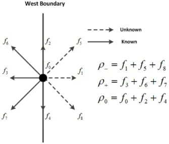
Referring to Figure 7, the contributors to the macroscopic density at a lattice point

can be grouped into three categories: those stationary or parallel to the boundaryρ0-f0,f2,

andf4in this case; those known density distributions pointed into the boundaryρ+-f3,f6,

andf7; and those pointed out from the boundaryρ−-f1,f5andf8. Every straight boundary

will have this grouping. Comparing this with Equation 11, it can be seen that Equation 20 is an identity. Additionally, considering the lattice velocities it is easy to demonstrate that the velocity component perpendicular to the straight boundary can be expressed as in Equation 21.

ρ=ρ−+ρ0+ρ+ (20)

ρu⊥=ρ+−ρ− (21)

Given Equations 20 and 21, given either the value for the velocity component into the

domain,u⊥ orρ, it is always possible to determine the other using only the density

(42)

Figure 7: Groups of density distributions on west boundary lattice point. Equations 22 and 23. ρ= 1 1 +u⊥ (2ρ++ρ0) (22) u⊥ =−1 + (2ρ++ρ0) ρ (23)

Once the value for ρ and u are known on the boundary, this information can be used to

judiciously assign values either to the unknown density distributions as in the Zou-He type boundary conditions [30] or, in the case of the regularized boundary conditions introduced in [31], to all distributions.

a. Zou-He Boundaries

The Zou-He scheme for prescribed pressure or velocity seek to find suitable values only for the unknown density distributions at the boundary lattice point. For this ex-ample, the case of a prescribed-velocity boundary condition on the West domain boundary as depicted in Figure 7 will be used.

(43)

For the condition depicted, when accounting for the prescribed velocity on

the boundary, there remain four unknowns: ρ, f1, f5 andf8. Balanced against these four

unknowns is the known relation for density given in Equation 11, and two equations for momentum given by Equation 12. In order to provide closure, a fourth relationship is nec-essary. The Zou-He boundary conditions develop this relationship by assuming “bounce-back” of the non-equilibrium part of the density distribution directed perpendicular to the boundary. In this case, this gives us Equation 24.

f1−f1neq =f3 −f3neq (24)

Applying Equation 10 along with the knownρanduand appropriate lattice vectorse1and

e3 and weightsw1,w3, the above relation simplifies to Equation 25

f1 =f3+

2

3ρux (25)

In two dimensions, this provides closure and values of the remaining unknown density distribution functions can be determined. For this example, the expressions are given as Equation 26 and Equation 27.

f5 =f7+ 1 2(f4−f2) + 1 2ρuy+ 1 6ρux (26) f8 =f6 − 1 2(f4−f2)− 1 2ρuy + 1 6ρux (27)

For prescribed pressure, the procedure is the same, except that givenρ, we solve foru⊥

-in this caseux.

For three dimensions, there are still more unknowns; using the D3Q15 lat-tice and applying a boundary condition to the west domain boundary, In addition to one of

ρoru⊥, there are five density distributions that are unknown: f1,f7,f9,f11 andf13. In the

(44)

The idea demonstrated in [32] is to apply the non-equilibrium bounce-back

as used in Equation 24 to all unknown density distribution values relative to the known

density distribution in the opposite direction. If we adopt the convention that for a given

density distributionfk,f_k¯ connotes the density distribution traveling in the opposite

direc-tion, andfkis an unknown density distribution, this is shown in Equation 28 for the D3Q15

lattice.

fk =f_k¯+ f_keq−f_k_¯eq ,k∈ {1,7,9,11,13} (28)

In order to correct for momenta in the plane of the boundary—for this example, in theyand

zdirections—an adjustment is applied to the density distributions that are not perpendicular

to the boundary, which is shown in Equation 29 for the D3Q15 lattice.

fk =fk+

1

4[eky(f3−f4) +ekz(f5−f6)] ,k ∈ {7,9,11,13} (29)

Putting this all together, we arrive at Equations 30 and 31.

f1 =f2+ 2 3ρinux (30) fk =f¯_k+ 1 12ρinux− 1 4[eky(f3 −f4) +ekz(f5−f6)] ,k∈ {7,9,11,13} (31)

For other lattice types and other boundaries, the same general prescription is followed.

b. Regularized Boundaries

For regularized boundary conditions, introduced in [31] and discussed in more detail in [29], all particle distribution functions on boundary lattice points are replaced

based on values of ρ, u or Π(1) that are either specified by the boundary condition or

(45)

In the same fashion as with the Zou-He boundary condition, given either

ρ or u⊥, the other macroscopic variable can be determined based on the known values

offα. Once this is complete,feq

α is computed using Equation 10. Values for the unknown

density distribution function—fk—are initially estimated based on bounce-back of the

non-equilibrium parts as in Equation 28. Since we cannot know the non-non-equilibrium portion of

fk, we simply assign it to have the same non-equilibrium component as f_k¯ as shown in

Equation 32.

fk =f_keq+f_k¯−f_¯_keq (32)

The tensor Π is the second-order moment of the particle density populations and can be

expressed as in Equation 33. Π= q−1 X α=0 eαeαfα (33)

Equation 34 is used to reconstruct hydrodynamically consistent values for all fα on the

boundary lattice point,

fα =fαeq+

wα

2c4

s

Qα :Π (34)

whereQα =eαeα−c2sI,Ibeing the identity matrix. This method for boundary condition

application is appealing for its generality. The superior stability properties of this method is discussed at length in [29] and [31].

E. BODY FORCES

Many physical simulations require the application of a body force. Some simple examples would be a simulation that includes gravity; a simulation with an imposed dif-ferential pressure, where the pressure is included as a body force on the fluid particles; or a multi-component model where the interaction between particles of different species are

(46)

modeled by nearest-neighbor force inputs. The most common way to incorporate these forces is via an adjustment to the equilibrium velocity as given in Equation 35,

ueq =u+ ∆u (35)

where∆uis given by Equation 36.

∆u= τF

ρ (36)

Equation 36 can be understood heuristically by consideringF= ma =md_dtu with

the relaxation parameterτ taking the role of the differential in time.

F. SCALING

The goal of any numeric simulation is to obtain quantitative and qualitative results that can be applied to a particular physical system of interest. Much LBM literature is cast in “LBM units” where the distance between lattice points and the time for each time step is unity. This presents a clean palate on which to develop the theory, but leaves out the crucial details of how to tailor LBM simulation parameters so that the results can be related to a particular set of fluid conditions.

In previous sections, the equations relevant for staging and executing a LBM simu-lation were presented entirely in lattice units—where every time step is of unit length and the distance between any adjacent lattice sites is also of unit length. Since this basic system of units is generally unsuitable for physical problems, basic physical parameters given in some units of length and time must be re-scaled consistently so that these parameters can be converted into units suitable for incorporation into the LBM algorithm.

As an intermediate step, it is sometimes customary to rescale physical units to non-dimensional units. This is particularly useful in cases where knowledge of the system state in terms of some non-dimensional parameters such as the Reynolds number is needed.

(47)

The nondimensionalization and scaling scheme employed for this research is illustrated in Figure 8.

Figure 8: Scaling from physical units, to dimensionless units to LBM units.

G. EXAMPLE

In an attempt to clarify the discussion from this chapter, the LBM formulation of a model problem will be discussed in detail.

1. Problem Description

The procedures discussed in this chapter are summarized in the flowchart appearing in Figure 10. The problem to be considered is illustrated schematically in Figure 9. The problem involves flow within a two-dimensional channel around a cylindrical obstacle. Flow enters from the left boundary with a prescribed parabolic velocity and exits out the right boundary with a prescribed constant pressure. The top and bottom boundary are modeled as no-slip walls.

2. Scaling and Setup

The process of scaling for this example problem will be completed in two steps as

described in the section on scaling. First, a characteristic time scale T0 and length scale

L0 will be identified. For this problem of a cylindrical obstruction in two dimensional

channel flow, the natural choice is to use the conventions for Reynolds scaling where the characteristic length is the diameter of the cylinder. Therefore, the characteristic length in

(48)

Figure 9: Schematic diagram of channel flow example problem.

for an average fluid particle to traverse the diameter of the cylinder. For the assigned inlet boundary condition, the average fluid velocity is two-thirds of the maximum inlet velocity

of 0.5 _secm for the parabolic profile. Consequently, T0,p = _UL0₀,p_,p = 0₀._.2₅ = 0.4sec All of this

corresponds to a Reynolds number of 100, which is convenient to know when comparing the output of the LBM simulation against experimental data or benchmark values.

The second step is to decide how finely the reference time and space scales are

to be subdivided. For this example, the reference length L0 will be represented with 25

lattice points, so there are intervals in the reference length. In terms of dimensionless units,

L0 = 1. The conversion between dimensionless units and the LBM units is therefore:

LLBM =δx = ₂₅1₋₁ = 0.0417. To convert between a distance in terms of lattice units and a distance in physical units, one would multiply by both the conversion factors. Therefore,

the physical spacing of the lattice points is δx ×L0,p = 0.0083 m. Similarly the time

domain is discretized by deciding how many time steps will be used to traverse a single

unit of the reference time T0. For this problem, the reference time will be divided by

250 time steps, so δt = _NTo_t = ₂₅₀1 = 0.004 seconds. As with the spatial scaling, in

(49)

the scaling parameters between the Dimensionless units and LBM units in addition to the conversion between Physical and Dimensionless units. For this problem, those conversions areTP =TLBM×δt×T0 = 0.0016.

Once the spatial and temporal scaling factors are determined, the properly scaled LBM parameters must be determined from the given physical data.

a. Viscosity Scaling

In order to get dynamic LBM behavior that corresponds to the desired phys-ical fluid under the prescribed conditions, the temporal and spatial scaling factors need to

be applied to the specified fluid kinematic viscosityν. Sinceνhas units of m_sec2 the necessary

conversion can be accomplished via Equation 37.

νLBM=νPhysical× T0δt

(L0δx)

2 (37)

Carrying out this conversion for the specified fluid with the chosen

dis-cretization results in νLBM = 0.023. This is the value that is applied to Equation 14 to

find the LBM relaxation parameter. Doing so for this problem results in τ = 0.57 or

ω = 1.76

b. Velocity BC Scaling

This problem has a prescribed inlet velocity profile. The velocity is ex-pressed in terms of meters-per-second, which is not compatible with the unit system as-sumed when the LBM boundary conditions were developed. The velocity is simply scaled in accordance with Equation 38.

uLBM =uPhysical × T0δt

L0δx

(38) For this problem, this conversion reads:

u(0, y) = 3 4 1−(y−0.5) 0.5 × 0.0016 0.0083 = 0.144 1− (y−0.5) 0.5 .

(50)

This is the velocity that will be passed to the LBM time-stepping routine in order to set the prescribed velocity at the inlet lattice points.

c. Pressure BC Scaling

For this problem, the prescribed outlet pressure is set to 0 Pa. This is a relative pressure, of course, otherwise the density for lattice points at the outlet would need to be set to zero according to Equation 13. Since the prescribed pressure boundary

condition procedures are actually methods for enforcing a specificdensityat the boundary,

in order to employ the pressure boundary condition for evaluating pressure on the domain we must:

• Compute the pressure through the domain using Equation 11 and Equation 13 along

with the value ofcsapplicable for the lattice in use.

• Scale the computed pressure to physical units using Equation 39. In this step, one is

simply convertingc2

s to physical units.

• Adjust the pressure in physical units so that the boundary condition is satisfied as in

Equation 40. PPhysical =ρLBMc2s δxL0 δtT0 2 (39) P =PPhysical−PBoundary (40)

3. Initialization and Lattice Point Classification

As final steps before commencing the LBM time-stepping routine, the initial values

forfα must be established for all lattice points. Additionally, all boundary lattice points,

solid lattice points, and any other type of lattice point that will require special treatment must be identified. For this problem, we need only identify inlet nodes for the prescribed velocity boundary condition, outlet nodes for the pressure boundary condition as well as

(51)

solid nodes for the top and bottom boundary as well as the cylindrical obstruction. Each of these classes of lattice points will be treated with distinction during each time-step.

There is no solidly established means for establishing an initial condition. A

com-mon choice for many problems is to simply set the initial set offα for each lattice point

equal to the equilibrium density distribution as computed with Equation 10 to some pre-determined velocity and density distribution. This is shown in Equation 41 for the D2Q9 lattice. fα(x,0) =fαeq=ρwα 1 + 3 (eα·u0) + 9 2(eα·u0) 2₋ 3 2(u0 ·u0) (41)

Similarly, there is no standardized procedure for generating the lattice domain, identifying inlet and outlet lattice points or lattice points along solid boundaries. General-purpose, Open-source lattice-generating software that could carry out tasks such as these on more complex geometries do not seem to exist. For problems with simple geometry, as this example problem does, this task can be executed quite efficiently with simple searches based on lattice point geometric position. (e.g, all of the inlet lattice points can simply be

found by identifying all of those points that lie alongx= 0and wherey6= 0andy6= 1.

4. Time-Stepping

The basic time-stepping scheme is illustrated in the flowchart shown in Figure 10. Fluid nodes not on a boundary compute values for macroscopic density and velocity using

Equation 11 and 12. These values are used to compute feq

α using Equation 10. Using

the scaled relaxation parameter computed using Equations 37 and 14, perform the BGK relaxation using Equation 9. A visualization of the results after 50,000 time steps are shown in Figure 11. This represents approximately 80 seconds of physical time according to our time scaling factor computed above.

(52)

(53)

Figure 11: Velocity magnitude, pressure, and vorticity magnitude for example flow case after 50,000 time steps.

(54)

III. IMPLEMENTATION AND VALIDATION

In order to model fluid structure interactions with LBM and FEM, it is necessary to have available a reliable, flexible and powerful implementation of the LBM. It must first be reliable so that we can have some reasonable hope that the results obtained will be comparable to physical reality. It must be flexible so that a wide variety of simulations can be conducted, pertaining to different physical conditions of interest. It must be powerful so that these simulations can be refined for greater accuracy while still able to be completed in a reasonable amount of time.

In this chapter, a body of software tools, designed using the theory presented in Chapter II, is tested against a selection of standard benchmarks first for accuracy and then for performance. The following results are obtained from this work:

• The LBM software as implemented for this work reliably reproduces

re-sults obtained Poiseuille flow, lid-driven cavity, flow over a backward step and flow over a cylindrical obstruction for 2D.

• The LBM provides second-order convergence to the 2D Poiseuille flow

with appropriate boundary conditions and double precision arithmetic. A mixed-precision algorithm is introduced which allows similar second-order convergence while only storing single-precision data.

• The LBM is benchmarked for performance against recently published

im-plementations for 3D lid-driven cavity flow. It is shown that the software produced for this work has competitive performance with other single-workstation implementations recently produced.

A. POISEUILLE FLOW

The first test case is a two-dimensional flow case between parallel plates. The flow condition is depicted in Figure 12.

(55)

Figure 12: Poiseuille flow configuration.

Channel Width (2×b) 1.0 m

fluid density (ρ) 1000 Kg_m2

fluid viscosity (µ) 1 N-s_m2

Maximum inlet velocity (Umax) 0.015 m_s

Table 1: Geometry and fluid parameters for Poiseuille flow test case.

The solution to this problem is known to be a function of y only and is given in

Equation 42: u(y) =− 1 2µ dp dx b 2₋_y2 (42)

with _dxdp given as a function of maximum velocity and fluid viscosity in Equation 43

dp dx =−

2µ

b2umax. (43)

The maximum velocity is set by the inlet boundary condition. Specific fluid and flow conditions are presented in Table 1.

(56)

1. Solution with On-Grid Bounceback Boundary Conditions

For the LBM model of this problem, the D2Q9 lattice with LBGK dynamics was used along with Zou/He boundary conditions for the prescribed velocity on the west bound-ary and constant prescribed pressure on the east boundbound-ary. The initial lattice discretization was set so that 30 lattice points would span the channel entrance. The time step was set to

achieve a relaxation parameterω of 1.30. While refining the grid to test for convergence,

the time step was adjusted so as to maintain a constant relaxation parameter for all tests. The results are shown in Figure 13. As expected, first-order convergence is obtained for this style of boundary condition.

2. Solution with Half-Way Bounceback Boundary Conditions

The half-way bounce-back boundary condition was implemented and used in an identical set of tests. The goal of this step, in addition to showing the convergence proper-ties of the boundary condition, is to illustrate the second-order convergence properproper-ties of the LBM as a whole. Results for single precision are shown in Figure 14. It is clear from the figure that, for problems with modest accuracy and comparatively coarse lattice densities, second-order convergence is obtained. For more refined lattices, however, the expected convergence rate is lost in single-precision. To investigate the effect of the numerical pre-cision in which the software is written, an alternate implementation was generated utilizing double precision arithmetic for all LBM calculations. Results of this convergence test are shown in Figure 15. In order to avoid the cost of double precision computations a mixed precision LBM kernel was developed. Through an experimental analysis of the sources of error in the LBM computations, it was found that numerical results nearly identical to that obtained with full double precision computations could be obtained by conducting

only computation of f_αeq and collisions in double precision. Convergence results for this

computation are shown in Figure 16.

The mixed precision brings the accuracy of double precision with a lower cost for memory consumption and with better performance than a pure double precision compu-tation. The memory cost for working in double precision is simply twice that of single

(57)

(58)

Figure 14: Poiseuille flow convergence with half-way bounce-back boundary conditions in single precision.

Figure 15: Poiseuille flow convergence with half-way bounce-back boundary conditions in double precision.

(59)

Figure 16: Poiseuille flow convergence with half-way bounce-back boundary conditions using mixed-precision arithmetic.

precision. The relative computational performance of single, mixed and double precision are presented in Figure 17 for two-dimensional Poiseuille flow using the LBGK collision operator. For less refined lattices, the double precision performance is nearly identical to single precision and both are slightly higher than mixed precision. For more dense lattices the additional memory-bandwidth load of passing double precision operands to the com-putational routines becomes more important than penalties paid for type conversions and mixed precision outperforms double precision.

3. Stability and Accuracy

In the preceding section, it may have seemed arbitrary to have selected a constant

relaxation parameter ω = 1.25. This conclusion is partially correct insofar as there is

considerable flexibility as to how this value is picked. We recall from Chapter II that,

including effects of scaling in time and space, the fluid viscosity in LBM-units scales by δt

δ2

x

in accordance with Equation 37. Consequently, ifδx is reduced by a factor of 2,δtmust be

reduced by a factor of 4. With this refined time step, the number of time steps is increased by a factor of 4 for the fluid simulation, including the time required for the LBM simulation