ever, its effect has not been considered sufficiently in most traffic models and analyses, which are typically based on clear weather conditions. To the extent that rain affects traffic stream behavior, it would be expected to influence the occurrence and associated char-acteristics of flow breakdown episodes. As such, it is important to understand and quantify this effect in order to properly estimate the capacity and reliability of traffic facilities as well as to develop mit-igation strategies aimed at preventing or delaying the onset of flow breakdown.
Recently, several researchers have studied the impact of different weather conditions on traffic behavior. Rakha et al. quantified the impact of precipitation intensity and visibility under rain and snow on three key parameters, namely, free-flow speed, speed at so-called capacity, and jam density, confirming reductions in free-flow speed and speed at capacity with increasing rain and snow intensity (4). The reduction in free-flow speed reported in that and several other studies varies from 1.7% to 3.6% in light rain and 4.4% to 9.0% in heavy rain (4–7). Free-flow speed reductions may be attributed to a combi-nation of factors, such as wet surface, low visibility, and adjustment in driver behavior. With regard to weather effects on breakdown, the study by Brilon et al. appears to be the only one to have reported on a reduction (around 11%) in breakdown capacity between dry and wet road surfaces (8).
In this study, the effect of rain on flow breakdown is investigated with regard to three principal aspects: (a) probability of breakdown occurrence given the prebreakdown flow rate; (b) duration of the breakdown episode once it occurs; and (c) relation between post-breakdown and prepost-breakdown flow rates. The study relies on sev-eral years of loop detector data on freeway sections in multiple locations in California. The data are analyzed by using hazard-based duration modeling techniques along with other standard statis-tical methods. Separate models are estimated for rain versus no rain conditions, allowing (a) formal testing of whether rain significantly affects the occurrence likelihood and duration of breakdown episodes and (b) quantification of these effects for the selected test sites.
The main contribution of this paper arises from the importance of the breakdown phenomenon, its prevalence on congested urban free-ways, and the frequency with which rain is experienced in many parts of the country. This is among the few studies that focus on weather effects, specifically on flow breakdown, and it is possibly the first to do so by using data from the United States. It is also the first study to conduct formal statistical tests of significance of these effects and to study breakdown duration by using hazard-based techniques. As such, it adds to the body of work aimed at understanding weather effects on traffic flow and provides important insight and tools for devising measures to mitigate these effects.
Likelihood and Duration of
Flow Breakdown
Modeling the Effect of Weather
Jiwon Kim, Hani S. Mahmassani, and Jing Dong
19 The effect of rain on freeway flow breakdown behavior is investigated. Three aspects of flow breakdown are analyzed for rain versus no rain (clear) weather conditions. First, the probability of breakdown occurrence is examined by analyzing the distribution of prebreakdown flow rates observed immediately before the onset of traffic breakdown by using a survival analysis approach. At all study sections, a reduction with pre-breakdown flow rates is observed under rain conditions compared with distributions under no rain and confirms higher breakdown likelihoods at lower flows. Log likelihood ratio tests confirm the statistical significance of differences in the prebreakdown flow rate distribution parameters under rain compared with clear conditions. Second, breakdown duration is examined by estimating a semiparametric Cox proportional hazard model. With a rain event indicator set as an independent variable, the effect of rain on breakdown duration is observed. Rain during a down episode is found to increase its duration, whereas rain before break-down does not appear to affect duration. Finally, prebreakbreak-down and postbreakdown flow rates are compared. Overall, while a reduction in prebreakdown flow rates is observed because of rain, the flow drop between prebreakdown and postbreakdown is not much different between rain (3.9% to 12.0%) and no rain (7.8% to 12.7%) conditions.
Major freeways in many urban areas are likely to experience traffic flow breakdown during peak periods. Traffic breakdown can be understood as an abrupt transition from an uncongested state to a congested state (1), though recent findings in traffic science have uncovered richer nuances in the so-called phases that traffic might exhibit (2, 3). Traffic characteristics associated with flow breakdown and the factors thought to influence its occurrence have been explored by many researchers from a variety of perspectives. However, its highly stochastic nature has precluded the ability to predict its occur-rence at a given time and location other than in a probabilistic sense. As such, the breakdown phenomenon is now largely recognized as a stochastic event, amenable to analysis by using probabilistic and statistical approaches.
An important factor that contributes to the stochastic properties of traffic flow is weather. Rain, in particular, is one of the most com-mon changes in external environment that affects traffic flow.
How-Transportation Center, Department of Civil and Environmental Engineering, Northwestern University, 600 Foster Street, Evanston, IL 60208. Corresponding author: H. S. Mahmassani, [email protected].
Transportation Research Record: Journal of the Transportation Research Board, No. 2188,Transportation Research Board of the National Academies, Washington, D.C., 2010, pp. 19–28.
The rest of the paper is organized as follows. Definitions of essen-tial quantities needed to describe the breakdown process are presented in the second section, along with descriptions of the study sites and related data processing. In the third section, the likelihood of break-down occurrence at different flow levels is analyzed. Breakbreak-down duration is analyzed in the fourth section, followed by the relation of postbreakdown to prebreakdown flow rates in the fifth section. In the final section results are summarized and concluding comments are provided.
PROBABILISTIC DESCRIPTION OF FLOW BREAKDOWN
Flow breakdown does not necessarily occur at the same location, nor at the same prevailing flow level or nominal maximal flow, especially in the presence of adverse weather or incidents. A probabilistic approach has been adopted in previous studies (8–12); for example, Brilon et al. (8) and Dong and Mahmassani (12) view the prebreak-down flow rate as a random variable and estimate the probability of flow breakdown at a given flow (demand) level. Traditionally, the term “capacity” has been used to indicate the maximum flow rate that can reasonably be expected to pass through a section of a roadway (8). However, because breakdown occurs at flows that may be lower or higher than the traditionally accepted (engineering) capacity, the flow rate observed immediately before traffic breaks down is referred to as the “prebreakdown flow rate” in this paper to avoid terminological confusion (12).
Figure 1 depicts time series of 5-min averages of flow and speed for one of the study locations, I-280N in South San Francisco, Cal-ifornia (13). With reference to Figure 1, the following quantities are defined:
Definition 1 (prebreakdown flow rate, qp). The flow rate, expressed
as a per lane equivalent hourly rate, observed immediately before the onset of traffic breakdown.
Definition 2 (postbreakdown flow rate, qb). The average flow rate,
expressed as a per lane equivalent hourly rate, observed after the onset of breakdown and before traffic recovers.
20 Transportation Research Record 2188
Flow Breakdown Detection Criteria
In previous research, flow breakdown is detected on the basis of a considerable speed drop from free-flow speed between two consec-utive time intervals. The speed drop between two consecconsec-utive time intervals (i.e., minimum speed difference) and the time duration over which low speed is sustained (i.e., minimum breakdown dura-tion), when used together, have also been suggested as an appropri-ate set of criteria (8, 12). Typically a threshold speed that divides congested and uncongested states is specified according to traffic data from a study section, and this threshold is viewed as a constant over time. While one might conveniently use free-flow speed or posted speed limit as the prebreakdown reference against which to measure the drop, it is preferable to use the actual (measured) pre-vailing free mean speed, especially on rainy days when the mean free speed tends to be lower than on clear days. In this study, the daily average speed in the free-flowing state is measured and used as a pre-vailing free mean speed (Vf) for that day (Figure 1). After
examin-ing 5-min volume and speed data (13), an appropriate speed drop is determined as 10 mph; the speed 10 mph lower than the prevailing free mean speed is then taken as the threshold speed (Vth) to separate uncongested and congested phases. As shown in Figure 2 in the speed–flow diagrams for both clear and rainy days for a study section in South San Francisco, the 10 mph threshold identifies successfully the breakdown state for that section.
However, because the speed drop does not occur sharply in all cases, it is useful to confirm the occurrence of breakdown by using an additional criterion. One possibility is to use occupancy in con-junction with speed. After experimentation with various study loca-tions and weather condiloca-tions, sustained duration of the lower speed following a drop was used in this study. Accordingly, the start and end of breakdown are defined as follows:
Definition 3 (start of breakdown). If speed in time interval iis above a threshold speed and speed in the next time interval i+1 is below the threshold speed, and low speed (below the threshold speed) is sustained for at least 15 min (the next three intervals), breakdown is assumed to start in time interval i+1, and the flow rate in time interval iis defined as prebreakdown flow rate qp.
Speed
Flow Rate
Occupancy
Precipitation Intensity Level Occupancy (%) Speed (mph) 0 20 40 60 80 100 Flows (v p h p l) Time of Day (hr) 15:00 16:00 17:00 18:00 19:00 20:00 21:00 22:00 2500 1500 2000 1000 +RA RA -RA No Rain Vf Vth qp Breakdown Duration
FIGURE 1 Time series of flow rate and speed for freeway section on I-280N in South San Francisco at 5-min intervals.
Definition 4 (end of breakdown). If speed in time interval iis below a threshold speed and speed in the next time interval i+1 is above the threshold speed, and low speed has been sustained for the previous three intervals, breakdown is assumed to end in time interval i.
Study Sites and Data Collection Traffic Data
Traffic data collected for this study consist of vehicle volume counts, speed, and occupancy at 5-min intervals for five freeway sections in the San Francisco Bay Area of California. Details of the five data collection locations are listed in Table 1. Data were collected from the PeMS website (13). Only workday data based on 100% observed raw data (i.e., no imputed data) were used. To observe as many rainy days as possible, traffic data during rainy season in this area, namely, November to April from 2000 to 2009, were selected. To avoid flow breakdown resulting from spillback from downstream, the bottleneck where congestion started was selected after an examination of time-series spatial contour maps provided by the PeMS website.
Weather Data
The weather data used for all sites were obtained from the automated surface observing system (ASOS) stations located at airports. ASOS provides weather observations at 5-min intervals. Precipitation inten-sities are reported in three levels: light rain (denoted by −RA; up to 0.10 in./h), moderate rain (RA; 0.11 to 0.30 in./h), and heavy rain (+RA; more than 0.30 in./h). This study, however, does not
distin-guish different precipitation intensity levels and considers all of them as rain events. One major reason is that weather data for the study area do not include a sufficient number of high-intensity precipita-tion events. Furthermore, for several instances in which high precip-itation was observed, overall demand levels appeared to be lower, and traffic moved at substantially lower speeds, hence confounding the analysis of breakdown occurrence and duration. However, the three rain intensity levels are included in time-series plots in Figures 1 and 3 to allow visual inspection.
To combine separately collected 5-min weather data with traffic data without losing accuracy, traffic observations are restricted to be within 10 mi from the nearest ASOS station. In addition, days on which either traffic or weather data are missing are not included in the data set.
PROBABILITY OF BREAKDOWN OCCURRENCE: RAIN VERSUS NO RAIN
The prebreakdown flow rate (qp) and the breakdown flow rate (qb)
are viewed as random variables, with distribution functions FQp(qp) and FQB(qb), respectively. By definition, the prebreakdown flow
dis-tribution at flow rate q, FQp(q), expresses the probability that traffic breaks down at flow rates less than or equal to q(in the next time interval, for a given time discretization). In other words, 1 −FQp(q) represents the probability of flow rate sustaining at q, indicating the travel reliability at flow rate q.To obtain the prebreakdown flow rate distribution, statistical methods used for lifetime data (survival) analysis are used to estimate distribution functions on the basis of samples that include censored data (8, 12). In this case, data are coded as uncensored if the flow rate in time interval i(qi) is followed by
TABLE 1 Traffic Data Collection Locations
Section Route Abs. Post Mile Lanes Location No. of Breakdowns
1 I-280N 45.14 4 South San Francisco, Calif. 425
2 I-880S 41.54 5 Oakland, Calif. 386
3 SR-101N 487.65 3 Santa Rosa, Calif. 378
4 SR-101S 420.21 4 Burlingame, Calif. 537
5 SR-101N 413.81 4 San Mateo, Calif. 627
Vf Vth Vf Vth 70 mph 60 mph 44 mph 34 mph Traffic Breakdown Speed (mph) 0 20 40 60 80 100 Speed (mph) 0 20 40 60 80 100 Flow rate (vphpl) 0 500 1000 1500 2000 2500 Flow rate (vphpl) (a) (b) 0 500 1000 1500 2000 2500
FIGURE 2 Speed–flow diagrams for section of I-280N in South San Francisco for 5-min intervals on (a) clear and (b) rainy days.
breakdown (i.e., qi = qp) and censored if breakdown is not
observed at i+1 (which means that qi< qp). First, a nonparametric
method was applied to obtain the empirical cumulative distribution for each data set without relying on a particular mathematical form. Second, a parametric method was used to fit a known form to the observed data.
Nonparametric Method
The product limit (PL) method, a nonparametric approach developed by Kaplan and Meier is applied for generating survival functions for the study sites (12, 14). The PL estimator produces a survival step function that is based purely on the observed data. This method provides useful estimates of survival probabilities and a graphical presentation of the survival distribution. However, if the largest
obser-22 Transportation Research Record 2188
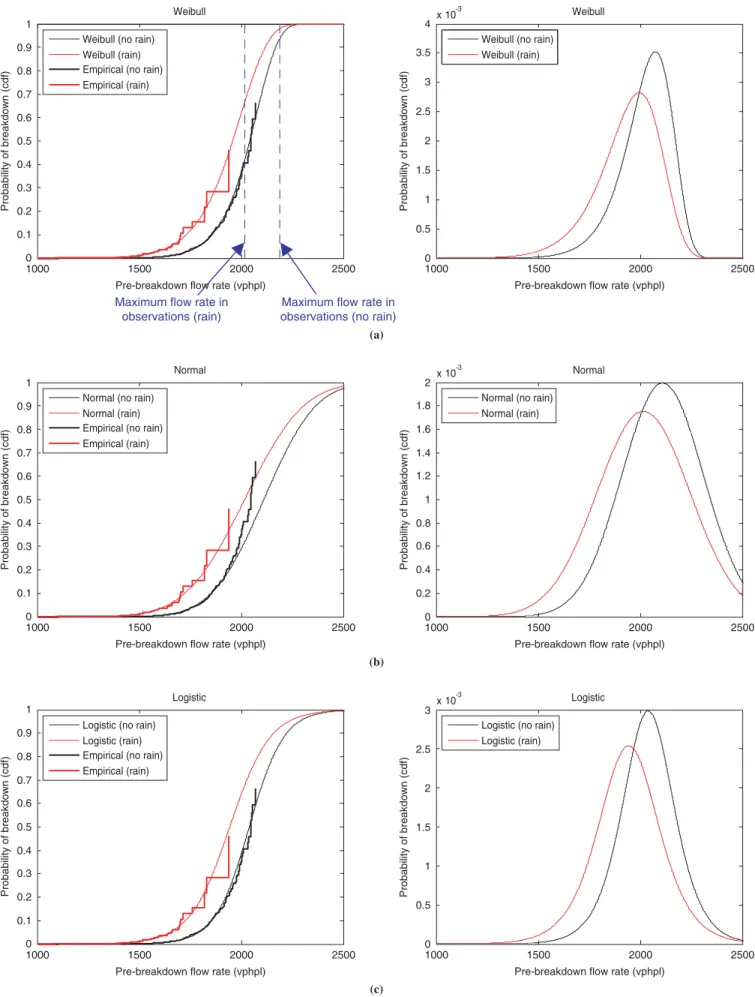
vation (the maximum flow rate observed in the sample) is censored, the PL estimate is undefined beyond this observation (15). Since breakdown may not have occurred at the maximum observed flow rate, the PL estimate provides only up to the largest uncensored data point, resulting in a cumulative probability of less than one at the maximum observed flow. This is presented in Figure 4a.
Parametric Method
To facilitate formal statistical comparison of the prebreakdown flow distributions under different weather conditions, it is useful to obtain an analytical expression that specifies the whole distribution function over the relevant flow range, with parameters that can be estimated for particular locations and weather conditions. Three types of func-tions, the Weibull, Gaussian (normal), and logistic distribufunc-tions, are 0 20 40 60 80 100 Speed (mph) 0 20 40 60 80 100 Speed (mph) 0 20 40 60 80 100 Speed (mph)
5AM 6AM 7AM 8AM 9AM 10AM 11AM 12PM 1PM 2PM 3PM 4PM 5PM 6PM 7PM 8PM 9PM 10PM 5AM 6AM 7AM 8AM 9AM 10AM 11AM 12PM 1PM 2PM 3PM 4PM 5PM 6PM 7PM 8PM 9PM 10PM 5AM 6AM 7AM 8AM 9AM 10AM 11AM 12PM 1PM 2PM
(c) (b) (a) 3PM 4PM 5PM 6PM 7PM 8PM 9PM 10PM 0 500 1000 1500 2000 2500 Flows (vph) 0 500 1000 1500 2000 2500 Flows (vph) 0 500 1000 1500 2000 2500 Flows (vph)
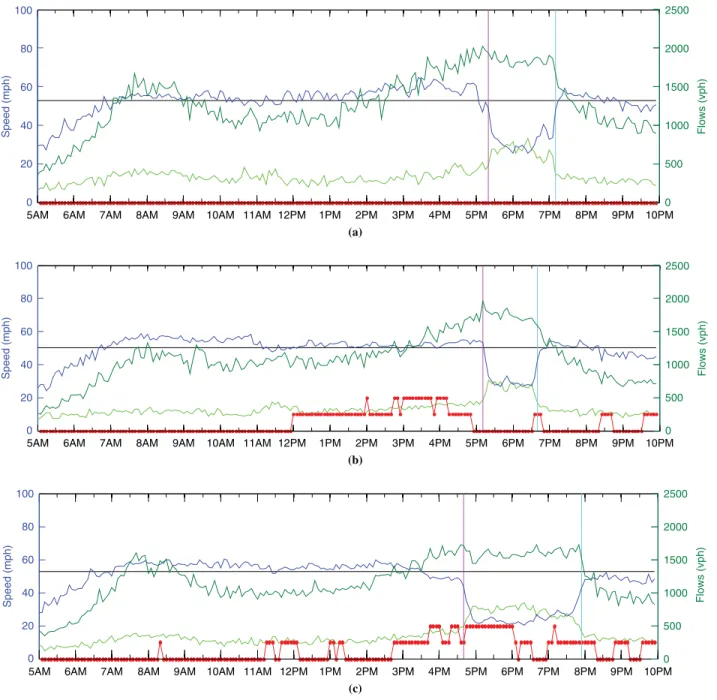
FIGURE 3 Time series traffic data from Section 1 on three Thursdays in January 2008 showing observations of breakdown duration under different weather conditions: (a) no rain, (b) prerain ⴝ1, and (c) postrain ⴝ1.
1000 1500 2000 2500 Pre-breakdown flow rate (vphpl)
1000 1500 2000 2500
Pre-breakdown flow rate (vphpl)
1000 1500 2000 2500
Pre-breakdown flow rate (vphpl)
1000 1500 2000 2500
Pre-breakdown flow rate (vphpl)
1000 1500 2000 2500
Pre-breakdown flow rate (vphpl)
(b)
(c) (a)
1000 1500 2000 2500
Pre-breakdown flow rate (vphpl) Weibull (no rain)
Weibull (rain) Empirical (no rain) Empirical (rain) 0 0.5 1 1.5 2 2.5 3 3.5 4
Weibull (no rain) Weibull (rain)
Normal Normal (no rain)
Normal (rain) Empirical (no rain) Empirical (rain) 0 0.2 0.4 0.6 0.8 1 1.2 1.4 1.6 1.8 2 x 10 -3 Normal
Normal (no rain) Normal (rain) 0 0.1 0.2 0.3 0.4 0.5 0.6 0.7 0.8 0.9 1 Logistic Probability of breakdown (cdf) 0 0.1 0.2 0.3 0.4 0.5 0.6 0.7 0.8 0.9 1
Probability of breakdown (cdf) Probability of breakdown (cdf)
0 0.1 0.2 0.3 0.4 0.5 0.6 0.7 0.8 0.9 1
Probability of breakdown (cdf) Probability of breakdown (cdf)
0 0.5 1 1.5 2 2.5 3 Probability of breakdown (cdf)
Logistic (no rain) Logistic (rain) Empirical (no rain) Empirical (rain)
x 10-3 Logistic
Logistic (no rain) Logistic (rain)
Maximum flow rate in observations (no rain) Maximum flow rate in
observations (rain)
FIGURE 4 Probability of breakdown (cumulative distribution function) under rain and no rain conditions in Section 4 for (a) Weibull, (b) Gaussian, and (c) logistic distribution.
tested (12). To estimate the parameters of the distribution functions, the maximum likelihood estimation method is used. The likelihood function (L) is given by Equation 1 (15):
where
n=number of observations,
δi=1 if uncensored and 0 otherwise, f(䡠)=probability density function, and F(䡠)=cumulative distribution function. Estimation Results
The parameters of the distribution function can be estimated by maximizing the likelihood function or its natural logarithm (log likeli-hood). The estimated parameters, along with the 95% confidence intervals and the log likelihood values, are listed in Table 2. Com-paring the log likelihood values, the best-fitted distribution varies with the location and associated weather condition. For Section 1, the logistic distribution provides the best fit under both rain and no rain conditions. For Sections 2 and 5, the Gaussian distribution pro-vides the best fit. For Sections 3 and 4, different distributions provide the best fit, with the Weibull best for Section 3 (rain) and Section 4 (no rain), and the Gaussian for Section 3 (no rain) and Section 4 (rain). Overall, the Gaussian distribution provides a reasonable fit at most locations, with the best log likelihood value at three sections under no rain and three sections under rain. However, the results might be different for other road types and other locations (8, 12). Figure 2 shows the cumulative distribution function and probability density function of the three models for Section 4 (SR-101S, Burlingame, California). The empirical curves calculated from the Kaplan–Meier PL method are also included on each cumulative distribution function plot. These plots clearly indicate that the probability of breakdown at a given flow rate under rain is higher than under no rain.
To ascertain whether these separate models for rain and no rain are significantly different from a pooled model, which is the model for all data including rain and no rain, a likelihood ratio test was con-ducted. The likelihood ratio test comparing two models (pooled model versus separate model) can be conducted by using the log likelihoods at convergence. The test statistic is as follows:
where LLRis the log likelihood for the pooled model, and LLUis the
sum of the log likelihood values for rain and no rain models. A null hypothesis (H0) is that parameters for rain versus no rain are the same. For example, in the case of the Weibull distribution, since this function has two parameters, scale (σ) and shape (s), the null hypoth-esisH0is that {σno_rain= σrainand sno_rain=srain} and thus the number of restrictions (degrees of freedom) is two. Test results are provided in Table 3. At all sections, χ2values are much greater than the crit-ical value (5.99) of the chi-square distribution at the 5% significance level, and indicate rejection of the restricted, null hypothesis model; in other words, separate models are significantly different from the model estimated with all data together. This confirms that the effect of rain on the likelihood of breakdown occurrence is significant.
Since LLUrepresents the combined log likelihood value for
sep-arate models, the distribution with the largest LLUcan be viewed as
the best model for a given section (Table 3). Table 4 summarizes the mean values of the prebreakdown flow rates under both no rain and χ2 2 2 = −
(
LLR−LLU)
( ) L f qi F q i n i i i =(
)
[
−(
)
]
= −∏
δ δ 1 1 1 1 i ( )24 Transportation Research Record 2188
rain conditions for the best-fit model for each section. The differ-ence between no rain and rain appears to vary within a narrow range, 51.5 to 97.4 vehicles per hour per lane (vphpl) (2.4% to 5.8% decrease with respect to no rain).
BREAKDOWN DURATION ANALYSIS
Breakdown duration is defined as the period between the occurrence of breakdown and recovery, as explained above. Duration analysis (i.e., survival analysis) is used to study the elapsed time until the occurrence of an event, or the duration of an episode. In particular, hazard-based models are applied to estimate the hazard function, which is the conditional probability that an event will occur in a time interval tgiven that the event has not occurred up to time t.If applied to the breakdown problem, the hazard function represents the prob-ability that breakdown will end at a duration tgiven that breakdown has continued up to a duration length t.Accordingly, a method to identify significant factors that affect the duration of breakdown is applied, namely a Cox proportional hazard (PH) model. In the Cox PH model, the hazard function is defined as follows:
where
h(t)=hazard function at time t;
h0(t)=baseline hazard, assuming all independent variables are zero;
xi=ith independent variable, i =1, . . . , K, and
βi=coefficient of ith independent variable, i =1, . . . , K.
Dividing both sides of above equation by h0(t), the hazard ratio or relative hazard is obtained as follows:
This ratio captures the expected change in the risk of the terminal event (i.e., end of breakdown) when a certain independent variable changes. If the hazard ratio is equal to one, the independent variable does not affect survival. If the ratio is greater than one, the indepen-dent variable is associated with decreased survival and vice versa. The PH approach assumes that the covariates, which are factors that affect the duration probabilities, act multiplicatively on some under-lying hazard function [h0(t)]. Furthermore, the start and end points of the breakdown episode are observed from the data (i.e., are uncen-sored); thus the PH model can be applied with no need to deal with the censoring problem.
Six explanatory variables are included in the initial specification of the duration models estimated for the breakdown episodes (Table 5). The effect of the rain factor is considered in two distinct periods: prebreakdown (prerain) and postbreakdown (postrain). The prerain variable is coded as one if more than three time intervals (15 min) experience rain within 1 h before the onset of breakdown (zero, other-wise). The postrain variable is coded as one if more than three time intervals (15 min) experience rain during the entire breakdown period (zero, otherwise).
An important feature of the Cox proportional model is the PH assumption, which assumes that the baseline hazard is a function of tbut that the covariates (Xs) are time-independent. It states that the hazard ratio (Equation 4) does not vary over time. To assess this assumption for the above covariates, a Schoenfeld residuals PH test
h t h t e x x k kx
(
)
(
)
= ( + + + ) 0 1 1 2 2 4 β β . . . β ( ) h t(
)
=h t(
)
e( x+ x+ + k kx) 0 1 1 2 2 3 i β β . . . β ( )Weather Distribution μ(Location) σ(Scale) s(Shape) Log Likelihooda Section 1 No rain Weibull — 2,223.8 23.9 −3,731.2 [2,211.1, 2,236.5] [22.9, 25.0] Gaussian 2,229.5 168.9 — −3,753.2 [2,211.9, 2,247.0] [160.1, 178.1] Logistic 2,175.7 71.8 — −3,709.5 [2,163.4, 2,188] [68.1, 75.7] Rain Weibull — 2,203.4 14.1 −375.0 [2,104.5, 2,306.9] [11.8, 16.9] Gaussian 2,250.1 286.2 — −375.8 [2,135.9, 2,364.2] [237.2, 345.3] Logistic 2,124.2 114.2 — −374.5 [2,048.0, 2,200.5] [95.4, 136.6] Section 2 No rain Weibull — 1,489.8 15.8 −3,314.4 [1,465, 1,514.9] [14.8, 16.8] Gaussian 1,523.9 178.2 — −3,308.7 [1,496.4, 1,551.3] [166.7, 190.4] Logistic 1,441.8 70.9 — −3,322.3 [1,422.5, 1,461.1] [66.5, 75.5] Rain Weibull — 1,421 13.5 −325.0 [1,336.5, 1,510.9] [10.9, 16.7] Gaussian 1,438.2 184.1 — −323.9 [1,350.5, 1,525.9] [148, 229] Logistic 1,367.1 76.9 — −326.3 [1,302.6, 1,431.5] [62.2, 95] Section 3 No rain Weibull — 1,654.8 18.8 −2,789.2 [1,636.5, 1,673.4] [17.7, 19.9] Gaussian 1,674.6 164.6 — −2,787.7 [1,652.1, 1,697] [154.3, 175.5] Logistic 1,617.5 69.4 — −2,791.2 [1,601.5, 1,633.4] [65.2, 73.8] Rain Weibull — 1,559.2 15.9 −525.2 [1,512.5, 1,607.4] [13.8, 18.3] Gaussian 1,577.2 177.4 — −525.7 [1,522, 1,632.3] [152.8, 206] Logistic 1,519.1 75.7 — −525.8 [1,479.7, 1,558.4] [65.5, 87.6] Section 4 No rain Weibull — 2,079.7 19.9 −4,299.9 [2,062.4, 2,097.1] [19, 20.9] Gaussian 2,110.1 200.1 — −4,309.7 [2,088.3, 2,131.9] [190, 210.6] Logistic 2,039.4 83.8 — −4,300.1 [2,024.2, 2,054.6] [79.7, 88] Rain Weibull — 2,005.1 15.4 −380.1 [1,931, 2,082] [13, 18.2] Gaussian 2,015.7 227.6 — −379.5 [1,929.6, 2,101.9] [189.4, 273.5] Logistic 1,943.5 98.5 — −380.3 [1,880.1, 2,006.9] [82.4, 117.9] Section 5 No rain Weibull — 1,812 13.8 −5,368.4 [1,785.5, 1,838.9] [13.1, 14.5] Gaussian 1,843 236.1 — −5,357.0 [1,814.9, 1,871.1] [224.1, 248.8] Logistic 1,736 94.4 — −5,380.9 [1,716.1, 1,756] [89.8, 99.3] Rain Weibull — 1,773.4 10.6 −662.0 [1,679.1, 1,872.9] [9.1, 12.3] Gaussian 1,778.5 271.5 — −660.7 [1,688.1, 1,868.9] [233.2, 316.2] Logistic 1,674.7 113.5 — −664.8 [1,608.5, 1,741] [97.9, 131.6]
NOTE: Numbers in brackets are 95% confidence intervals; — = not applicable.
a
is used (16, 17). The test results indicate that the first four traffic-related quantities (see Table 5) have some instances in which violation could not be rejected for certain sections at the 5% significance level. However, no variable is consistently found to violate the PH assumption for all sections. Furthermore, the PH assumption holds for both prerain and postrain indicator variables for all five sections. The estimation results for the final Cox model specification are presented in Table 6. Only three variables are retained in the final specification. Other variables were dropped from the specification because they were found to not exert a statistically significant effect on breakdown duration. The results in Table 6 also indicate that pre-rain is not statistically significant, with p-values that are greater than the 0.05 significance threshold. Contrary to prerain, postrain turns out to have a significant effect on breakdown duration. All p-values are less than 0.05 and the hazard ratio, which is the exp(β) value, is in the range of 0.339 to 0.529 (47.1% to 66.1% reduction in hazard function with respect to the baseline hazard). For example, if exp(β) is 0.339, the postrain indicator variable decreases the hazard of ter-minating breakdown by 66.1%, and thus lengthens the breakdown duration. For all five sections, rain occurrence during breakdown increases the latter’s duration compared to the breakdown duration on clear days. In addition to rain factors, it is found that postbreakdown speed increases the hazard in the range of 5.5% to 27.5% and conse-quently shortens the duration. For all sections, the lower the average speed after breakdown, the longer the breakdown episode will be.
One graphical example related to the above inference is provided in Figure 3, which illustrates the time series of traffic and weather data for Section 1 for three Thursdays in January 2008. With simi-lar flow patterns up to the breakdown onset point, breakdown dura-tions under no rain (3a) and prerain (3b) conditions appear nearly
26 Transportation Research Record 2188
the same; however, under the postrain condition (3c), breakdown duration increases to about twice the length of the former two cases.
PREBREAKDOWN AND POSTBREAKDOWN FLOW RATE UNDER RAIN VERSUS NO RAIN
In this section, the effect of rain on breakdown phenomena based on the actual breakdown observations (uncensored data only) is dis-cussed. For each section, prebreakdown flow rate, postbreakdown flow rate, and duration of breakdown under rain versus no rain are averaged. Comparisons between prebreakdown and postbreakdown flow rates and breakdown duration under rain versus no rain are presented in Table 7. The notations used in Table 7 are as follows:
qp,nr=prebreakdown flow rate under no rain, qb,nr=postbreakdown flow rate under no rain, qp,ra=prebreakdown flow rate under rain, and qb,ra=postbreakdown flow rate under rain.
To investigate the effect of rain more clearly, only cases in which it started raining before breakdown and continued during breakdown were included in the “rain” group. In Table 7, the columns labeled qp,nr−qb,nrand qp,ra−qb,rarepresent the flow drop before and after breakdown under no rain and rain, respectively. The mean flow drop due to breakdown appears similar in both weather cases, showing a 7.8% to 12.7% reduction under no rain and a 3.9% to 12.0% reduc-tion in rain. However, for each secreduc-tion, the flow drop under rain is TABLE 3 Likelihood Ratio Test Results
Degrees of Freedom: 2
Weibull Gaussian Logistic
Test Test Test Section LLR LLU Statistic p-Value LLR LLU Statistic p-Value LLR LLU Statistic p-Value
1 −4,164.5 −4,106.2 116.7 .0000 −4,213.1 −4,129.1 168.1 .0000 −4,142.9a −4,084.0 117.8 .0000 2 −3,658.5 −3,639.4 38.1 .0000 −3,652.9 −3,632.6a 40.7 .0000 −3,667.2 −3,648.6 37.2 .0000 3 −3,357.1 −3,314.4 85.4 .0000 −3,360.0 −3,313.3a 93.4 .0000 −3,358.9 −3,317.0 83.7 .0000 4 −4,711.5 −4,680.0a 63.0 .0000 −4,724.3 −4,689.2 70.3 .0000 −4,711.3 −4,680.4 61.7 .0000 5 −6,069.9 −6,030.4 79.0 .0000 −6,060.9 −6,017.7a 86.4 .0000 −6,082.9 −6,045.7 74.3 .0000
NOTE: Degrees of freedom = 2.
aDistribution with largest LL
Ucan be viewed as best model for a given section.
TABLE 4 Comparison of Mean Values of qpBetween No Rain and Rain
Best-Fitting μnr− μra
Section Model Mean,μnr Mean,μra (as % of μnr)
1 Logistic 2,175.7 2,124.2 51.5 (2.4) 2 Gaussian 1,523.9 1,438.2 85.7 (5.6) 3 Gaussian 1,674.6 1,577.2 97.4 (5.8)
4 Weibull 2,024.3 1,937.7 86.6 (4.3)
5 Gaussian 2,110.1 2,015.7 94.4 (4.5)
NOTES: nr =no rain; ra =rain.
TABLE 5 Variable Definitions for Breakdown Duration Models Variable Variable Description
Duration Time period between occurrence and recovery of breakdown [dependent variable]
qp Prebreakdown flow rate [continuous variable] qb Postbreakdown flow rate (average flow rate during
breakdown) [continuous variable]
vp Prebreakdown speed (speed at prebreakdown flow rate) [continuous variable]
vb Postbreakdown speed (average speed during breakdown) [continuous variable]
Prerain 1 if it rains before breakdown, 0 otherwise [dummy variable] Postrain 1 if it rains during breakdown, 0 otherwise [dummy variable]
always less than that in no rain. The column labeled qp,nr−qp,ra rep-resents the difference between prebreakdown flow rate under rain and no rain. The mean reduction in prebreakdown flow because of rain appears to remain in a certain range, from 90 to 297 vphpl (8.1% to 15.3%). Additionally, by comparing the mean duration of obser-vations under no rain and rain, the average increase in breakdown duration because of rain ranges from 34.8% to 43.8%, as presented in the far-right column of Table 7.
CONCLUSION
This study investigated the effect of rain on three aspects of flow breakdown: the probability of breakdown, breakdown duration, and the relation between prebreakdown and postbreakdown flow rates. Using 5-min interval traffic data (flow, speed, and occupancy) and weather data obtained over several years from the San
Fran-cisco Bay Area in California, various statistical analyses were conducted.
Probability of Breakdown
Viewing the prebreakdown flow rate as a random variable, the like-lihood of breakdown occurrence at different flow rates was esti-mated for both rain and clear conditions. The empirical distribution was calculated by using the nonparametric product–limit method, while parametric models (Weibull, Gaussian, and logistic), estimated by using the maximum likelihood method, formed the basis of the statistical analysis.
• The distribution providing the best fit to the data differs over study sections and weather conditions; the Gaussian distribution provides the best fit in six cases (three rain models and three no rain models) of 10. TABLE 6 Parameters of Cox PH Model
95.0% CI for exp(β) Variable Section β SE z-Statistic df p-Value exp(β) Lower Upper
vb 1 0.144 0.014 10.054 1 0.000 1.155 1.123 1.187 2 0.107 0.010 10.268 1 0.000 1.113 1.090 1.136 3 0.086 0.011 7.635 1 0.000 1.090 1.066 1.114 4 0.243 0.023 10.445 1 0.000 1.275 1.218 1.334 5 0.053 0.006 8.682 1 0.000 1.055 1.042 1.067 Prerain 1 −0.004 0.240 −0.018 1 0.985 0.996 0.622 1.593 2 0.136 0.239 0.569 1 0.569 1.145 0.718 1.828 3 0.413 0.278 1.482 1 0.138 1.511 0.875 2.608 4 0.134 0.319 0.421 1 0.674 1.144 0.612 2.137 5 −0.057 0.180 −0.317 1 0.751 0.944 0.664 1.344 Postrain 1 −0.990 0.241 −4.100 1 0.000 0.372 0.232 0.597 2 −0.637 0.212 −3.000 1 0.003 0.529 0.349 0.802 3 −0.804 0.275 −2.922 1 0.003 0.448 0.261 0.768 4 −1.080 0.273 −3.962 1 0.000 0.339 0.199 0.579 5 −0.854 0.175 −4.887 1 0.000 0.426 0.302 0.600
NOTES: SE =standard error; df =degrees of freedom; CI =confidence interval.
TABLE 7 Comparison of Mean Prebreakdown and Postbreakdown Flow Values
(8) % Average
(3) (6) (7) Increase in
(1) (2) qp,nr−qb,nr (4) (5) qp,ra−qb,ra qp,nr−qp,ra Breakdown Section qp,nr qb,nr ((1) −(2)) qp,ra qb,ra ((4) −(5)) ((1) −(4)) Duration
1 1,950 1,797 153 1,652 1,587 65 297 40.9 149 118 (−7.8%) 214 183 (−3.9%) (−15.3%) 2 1,103 1,012 91 1,014 929 83 90 35.8 100 86 (−8.3%) 86 106 (−8.2%) (−8.1%) 3 1,349 1,182 167 1,239 1,090 149 110 41.2 117 86 (−12.4%) 137 81 (−12.0%) (−8.2%) 4 1,723 1,571 152 1,544 1,430 114 179 34.8 156 122 (−8.8%) 156.0 130 (−7.4%) (−10.4%) 5 1,295 1,132 164 1,158 1,028 130 138 43.8 133 117 (−12.7%) 134 107 (−11.2%) (−10.6%)
NOTES: Numbers in italics are standard deviation. Numbers in parentheses are percent reduction with respect to former term.
No Rain Rain
• For all sections, the probability of breakdown at a given flow is higher under rain than under no rain; the effect of rain was shown to be statistically significant by performing likelihood ratio tests.
Breakdown Duration
A Cox PH model was used to study the factors that affect the duration of breakdown episodes. The analysis and estimated model results indicate that
• Rain during the breakdown episode increases breakdown dura-tion significantly,
• Rain before breakdown does not significantly affect breakdown duration for the locations tested,
• The mean increase in breakdown duration of actual observations because of the rain ranges from 34.8% to 43.8%, and
• The lower the average speed after breakdown, the longer the breakdown episode.
Prebreakdown and Postbreakdown Flow Rates
The average values of service flow rates before and after (during) breakdown were compared between rain and no rain for each section.
• Mean flow drop before and after breakdown with respect to prebreakdown flow rates ranges from 7.8% to 12.7% under no rain and from 3.9% to 12.0% under rain.
• The prebreakdown flow rate under rain is lower than under no rain for all sections; the mean reduction for actual breakdown instances is found to be 8.1% to 15.3%.
This paper demonstrates the effect of rain on the likelihood of breakdown occurrence and its duration. However, while analyzing thousands of breakdown cases over various locations, the authors have encountered considerable variability in breakdown behavior under different weather conditions. In particular, weather may induce other adjustments in traffic patterns. For instance, heavy rain may decrease the overall demand level, thereby preventing breakdown from occurring even during peak hours. In addition, because it reduces the prevailing free mean speed itself, sharp drops in speed may not be readily observed, making the detection of breakdown difficult. As other weather researchers have noted (4), visibility may also have a large impact on breakdown. However, because low visibility typi-cally accompanies heavy rain, its effect may be confounded with the rain effect. Nonetheless, a more complete understanding of the inter-action of weather with various factors that affect the occurrence and characteristics of this highly volatile phenomenon requires consider-able additional observation at different locations and under various conditions.
ACKNOWLEDGMENTS
The material presented in this paper is based in part on work funded by the U.S. Department of Transportation under a contract to North-western University’s Transportation Center through a subcontract to SAIC, Inc. The authors acknowledge the assistance of Roger B. Chen in the estimation of the duration models included in the analysis and
28 Transportation Research Record 2188
the helpful comments on the overall project provided by Roemer Alfelor of FHWA, Tim Lutrell of SAIC, Inc., and Byungkyu (Brian) Park of the University of Virginia.
REFERENCES
1. Lorenz, M. R., and L. Elefteriadou. Defining Freeway Capacity As Function of Breakdown Probability. In Transportation Research Record: Journal of the Transportation Research Board, No. 1776,TRB, National Research Council, Washington, D.C., 2001, pp. 43–51.
2. Kerner, B. The Physics of Traffic: Empirical Freeway Pattern Features. In Engineering Applications and Theory,Springer, Heidelberg, Ger-many, 2004.
3. Schönhof, M., and D. Helbing. Empirical Features of Congested Traf-fic States and Their Implications for TrafTraf-fic Modeling. Transportation Science,Vol. 41, No. 2, 2007, pp. 135–166.
4. Rakha, H. A., M. Farzaneh, M. Arafeh, and E. Sterzin. Inclement Weather Impacts on Freeway Traffic Stream Behavior. In Transportation Research Record: Journal of the Transportation Research Board, No. 2071,Transportation Research Board of the National Academies, Wash-ington, D.C., 2008, pp. 8–18.
5. Lamm, R., E. M. Choueiri, and T. Mailaender. Comparison of Operat-ing Speeds on Dry and Wet Pavements of Two-Lane Rural Highways. In Transportation Research Record 1280,TRB, National Research Council, Washington, D.C., 1990, pp. 199–207.
6. Ibrahim, A. T., and F. L. Hall. Effect of Adverse Weather Conditions on Speed-Flow-Occupancy Relationships. In Transportation Research Record 1457,TRB, National Research Council, Washington, D.C., 1994, pp. 184–191.
7. Highway Capacity Manual.TRB, National Research Council, Washing-ton, D.C., 2000.
8. Brilon, W., J. Geistefeldt, and M. Regler. Reliability of Freeway Traffic Flow: A Stochastic Concept of Capacity. In Transportation and Traffic Theory: Flow, Dynamics and Human Interaction—Proceedings of the 16th International Symposium on Transportation and Traffic Theory (H. S. Mahmassani, ed.), Elsevier, New York, 2005.
9. Persaud, B., S. Yagar, and R. Brownlee. Exploration of the Break-down Phenomenon in Freeway Traffic. In Transportation Research Record 1634,TRB, National Research Council, Washington, D.C., 1998, pp. 64–69.
10. Kerner, B. S. Theory of Breakdown Phenomenon at Highway Bottle-necks. In Transportation Research Record: Journal of the Transportation Research Board, No. 1710,TRB, National Research Council, Washington, D.C., 2000, pp. 136–144.
11. Evans, J. L., L. Elefteriadou, and N. Gautam. Probability of Breakdown at Freeway Merges Using Markov Chains. Transportation Research Part B,Vol. 35, 2005, pp. 237–254.
12. Dong, J., and H. S. Mahmassani. Flow Breakdown, Travel Reliability and Real-Time Information in Route Choice Behavior. In Proceedings of the 18th International Symposium on Transportation and Traffic Theory(W. Lam, S. C. Wong, and H. Lo, eds.), Springer, 2009. 13. PeMS—Freeway Performance Measurement System. http://pems.eecs.
berkeley.edu/. Accessed July 30, 2009.
14. Kaplan, E. L., and P. Meier. Nonparametric Estimation from Incomplete Observations. Journal of the American Statistical Association,No. 53, 1958, pp. 457–481.
15. Washington, S., M. G. Karlaftis, and F. L. Mannering. Statistical and Econometric Methods for Transportation Dada Analysis.CRC Press, Boca Raton, Fla., 2003.
16. Lee, E. T., and J. W. Wang. Statistical Methods for Survival Data Analy-sis.Wiley, Hoboken, N. J., 2003.
17. Schoenfeld, D. Partial Residuals for the Proportional Hazards Regression Model. Biometrika,Vol. 69, No. 1, 1982, pp. 239–241.
The authors are solely responsible for all contents in this paper. The views and opinions expressed are those of the authors and do not necessarily reflect the views of the sponsoring or performing agencies.