Accepted Manuscript
Production Planning in Additive Manufacturing and 3D Printing
Qiang Li , Ibrahim Kucukkoc , David Z. Zhang
PII: S0305-0548(17)30013-8
DOI: 10.1016/j.cor.2017.01.013
Reference: CAOR 4177
To appear in: Computers and Operations Research
Received date: 3 June 2016 Revised date: 28 October 2016 Accepted date: 24 January 2017
Please cite this article as: Qiang Li , Ibrahim Kucukkoc , David Z. Zhang , Production Planning in Additive Manufacturing and 3D Printing, Computers and Operations Research (2017), doi:
10.1016/j.cor.2017.01.013
This is a PDF file of an unedited manuscript that has been accepted for publication. As a service to our customers we are providing this early version of the manuscript. The manuscript will undergo copyediting, typesetting, and review of the resulting proof before it is published in its final form. Please note that during the production process errors may be discovered which could affect the content, and all legal disclaimers that apply to the journal pertain.
ACCEPTED MANUSCRIPT
Highlights Production planning problem in additive manufacturing and 3D printing is introduced
The mathematical model of the problem is developed and coded in CPLEX
Two heuristics are proposed and explained through a numerical example
Optimal and heuristic solutions are provided for the newly generated test problems
ACCEPTED MANUSCRIPT
Production Planning in Additive Manufacturing and 3D Printing
Qiang Li a,c, Ibrahim Kucukkoc a,b,*, David Z. Zhang a,c
a College of Engineering, Mathematics and Physical Sciences, University of Exeter, North Park Road, EX4 4QF Exeter, England, United Kingdom
b
Department of Industrial Engineering, Faculty of Engineering and Architecture, Balikesir University, Cagis Campus, 10145 Balikesir, Turkey
c The State Key Laboratory of Mechanical Transmissions, Chongqing University, Chongqing, 400044, China
[email protected], [email protected], [email protected]
Abstract
Additive manufacturing is a new and emerging technology and has been shown to be the future of manufacturing systems. Because of the high purchasing and processing costs of additive manufacturing machines, the planning and scheduling of parts to be processed on these machines play a vital role in reducing operational costs, providing service to customers with less price and increasing the profitability of companies which provide such services. However, this topic has not yet been studied in the literature, although cost functions have been developed to calculate the average production cost per volume of material for additive manufacturing machines.
In an environment where there are machines with different specifications (i.e. production time and cost per volume of material, processing time per unit height, set-up time, maximum supported area and height, etc.) and parts in different heights, areas and volumes, allocation of parts to machines in different sets or groups to minimize the average production cost per volume of material constitutes an interesting and challenging research problem. This paper defines the problem for the first time in the literature and proposes a mathematical model to formulate it. The mathematical model is coded in CPLEX and two different heuristic procedures, namely ‘best-fit’ and ‘adapted best-fit’ rules, are developed in JavaScript. Solution-building mechanisms of the proposed heuristics are explained stepwise through examples. A numerical example is also given, for which an optimum solution and heuristic solutions are provided in detail, for illustration. Test problems are created and a comprehensive experimental study is conducted to test the performance of the heuristics. Experimental tests indicate that both heuristics provide promising results. The necessity of planning additive manufacturing machines in reducing processing costs is also verified.
Keywords: production planning; additive manufacturing; 3D printing; scheduling; operations management; optimization
*
Corresponding author: Ibrahim Kucukkoc, Permanent Email: [email protected] Tel: +441392723613 (IK and QL); +441392723641 (D.Z.Z)
ACCEPTED MANUSCRIPT
1. IntroductionAdditive manufacturing (AM), also known as 3D printing (3DP), is the “process of joining materials to make objects from 3D model data, usually layer upon layer, as opposed to subtractive manufacturing methodologies, such as traditional machining” [1]. The development of AM technology started in the 1980s, and different AM processes have been developed, such as fused deposition modelling, laminated object manufacturing, stereo lithography and selective laser sintering, which are usually used as a means for rapid prototyping of non-metal materials. Laser engineered net shaping, electron beam melting and selective laser melting (SLM) – also known as direct metal laser sintering (DMLS) – are the most significant AM processes for rapid manufacturing, as opposed to prototyping, of metal materials. Detailed information on these AM processes have been given in previous works, see for example Coykendall et al. [2], Huang et al. [3], and Koff and Gustafson [4]. Compared to conventional manufacturing processes, AM processes carry several significant advantages, such as material efficiency, resource efficiency, part flexibility, production flexibility [3, 5] and direct kitting [6, 7]. These advantages empower AM as a unique competitor in production of small-batch products with complex structures and rapidly-changing designs [5]. A growing number of companies from various industries are trying to adopt AM/3DP technologies in the production of their products. As such, a series of issues in production planning of AM/3DP, particularly with SLM/DMLS facilities, are emerging due to the unique nature of this production process.
With the rapid development of material science and manufacturing technologies, AM (in particular SLM/DMLS) has shifted from making prototypes to direct part production (which is also known as direct digital manufacturing). Such a shift also leads to a new industrial revolution in the defense, aerospace, automotive and healthcare industries. As the AM technology is used directly to produce end-use metallic parts from powder materials, SLM/DMLS technology has become the dominant application of metallic AM processes, thanks to its high accuracy and performance in comparison to other metallic AM processes. The benefits of adopting SLM/DMLS have been captured in a variety of applications, spanning a number of industries and different stages of the product development lifecycle. The aerospace and defense industry, as an early adopter of AM technology, currently represents over 10% of the global AM market, and the metal AM
ACCEPTED MANUSCRIPT
sector alone has grown by over 70% in the last 15 years [8]. As reported by Coykendall et al. [2], NASA (National Aeronautics and Space Administration) used 70 additively-manufactured parts (such as flame-retardant vents, camera mounts and housings) for the Mars Rover test vehicles. Also, NASA has already trialed 3D printing on the International Space Station, which allows astronauts to print tools and parts in space exactly when needed [9]. Boeing had printed 22,000 components that are used in a variety of aircrafts by 2012. European Aeronautic Defense and Space (EADS) used DMLS to build an optimized design of bracket, which will be used in the Airbus A320; DMLS brought down the part’s weight by 64% while maintaining its strength and performance. General Electric used additively manufactured fuel nozzles as a single part, which previously involved the assembly of 20 different parts, in their LEAP engines. The parts are also reported to be five times more durable than those produced using conventional methods [2]. In the automotive industry, major manufacturers have been using 3DP for prototyping for years, and are poised to begin applying the process to produce parts directly. There is a growing number of applications for 3DP in surgery to produce implants such as cranial plates, jaws, and dentures with titanium, which perfectly match the human body.
The general production process of SLM/DMLS, as well as powder-bed based AM technology, is illustrated in Figure 1. The production with SLM/DMLS is job–based, and one or more parts with different heights can be produced simultaneously in one job. Firstly, a series of operations is needed to set up a new job, such as data preparation, filling of powder materials, adjustment of the AM machine, and filling up protective atmosphere. Afterwards, the job can be started. Thin powder layers with a typical thickness of between 20 µm and 60 µm are generated on a metallic base plate or the already-produced fraction of objects. The cross-sections of a sliced computer–aided-design file are subsequently scanned using a high power laser beam to densify the powder material [10]. These two processes, namely powder layering and laser melting, will alternate until all parts in the job are produced. The accumulated time spent on generating powder layers will be significant, especially when the thickness of each layer is smaller, even longer than the time spent densifying the powder materials in some cases. For example, given a part 300 mm high, and 15 seconds for generating each powder layer, the AM machine will spend more than 62 hours generating powder layers if the thickness of
ACCEPTED MANUSCRIPT
each layer is 20 µm. Finally, the parts produced in the job should be taken out from machine for post-processing, and the machine should be cleaned. The filters should also be replaced periodically in preparation for the next job. Time spent on setting up a new job and cleaning the AM machine usually ranges from one hour to several hours.
Figure 1. The production process of SLM/DMLS
Currently, the operating costs of SLM/DMLS is high due to its nature of the layer-upon-layer process. That is the major reason which prevents the extensive application of SLM/DMLS in industry. The high operation cost requires distributed parts to be centralized to increase utilization of the AM/3DP equipment. However, it is usually hard for individual companies to undertake the high investment and operating costs of centralization. Furthermore, the production requests of one company are usually far from filling the capacity of an AM/3DP machine, and the machines are mostly used for producing parts during the research and development (R&D) phase of creating new products. Therefore, it is recommended that distributed parts should be centralized to increase the utilization of the AM/3DP machines. Second, the nature of the layer-upon-layer process and job-based production makes it difficult to produce an optimal production schedule of parts. According to the production processes of SLM/DMLS described previously, only the time and costs spent on laser melting are directly related to the material volume of each part in the job. Time and costs spent on setting up a new job, powder layering, and cleaning of the machine are shared by all parts arranged in the same job. As mentioned previously, these shared time and costs are significant, especially when there are parts which are taller or built using thinner layers. For example, given a part 300 mm in height, 100 mm2 in production area and 6,000 mm3 in material volume, on a standard AM/3DP machine (whose details will be given in Section 3.2 for a numerical example) the production cost per unit volume of material will be 46.52 British
ACCEPTED MANUSCRIPT
Pound Sterling - GBP (according to the formulation which will be given in Section 3.2). However, this cost will be reduced to 5.16 GBP (about one ninth) if the remaining production area is assigned to other parts with the same specification of the given part. In doing so, the production cost per unit volume of material will change every time a new part is added into the job, and the final production cost cannot be determined until all the parts have been assigned. Furthermore, the production time of a job cannot be determined unless all the parts in a job have been assigned, which makes it difficult to get an optimal result when the delivery time of each part is considered. There are some production scheduling techniques for batch processes, see for example Lin et al [11], Mishra et al. [12] and Mendez et al. [13]. However, considering the unique and sophisticated production environment of SLM/DMLS, novel production planning models and optimization techniques are required to facilitate their application in industry.
As an emerging advanced manufacturing technology, AM technology has been studied extensively by academics and practitioners. However, researchers are mostly focused on the process and their applications in different industries, see for example, SmarTech [14], Cooper et al. [15], Khajavi et al. [16], and Koff and Gustafson [4]. Few pieces of research have been conducted for the calculation of cost structures in AM technology. Atzeni and Salmi [17] compared the production cost between SLS and traditional high-pressure die-casting and concluded that additive techniques can be economically convenient. Rickenbacher et al. [10] proposed an integrated cost model for SLM and found that the manufacturing time, as well as the set-up time (and therefore the total cost per part), was significantly reduced by simultaneously building up multiple parts. The cost models proposed in the past have also been discussed by Rickenbacher et al. [10]. Those cost models presented different methods for calculating the production cost of AM. Also, Hedenstierna et al. [7] addressed to order book management in 3D printing service operations for capacity smoothing. However, to the best of authors’ knowledge, no research has been conducted to address planning of production with AM technologies. In comparison with traditional manufacturing technologies, production with AM technology (in particular powder-bed based SLM/DMLS) is significantly different, where a novel method is needed to facilitate the utilization of AM machines efficiently and reduce production costs. The major distinction of production with a powder-bed based AM process is that the production cost and lead time are dynamically impacted by the
ACCEPTED MANUSCRIPT
combination of parts included in the same job, while some parts cannot be allocated to some machines due to capacity and maximum supported height/area characteristics. Therefore, it is hard to determine which combination of parts will be produced on which machine. The cost and time of a job may vary when a part with a particular height, production area, and material volume is added. In this environment, this paper aims to introduce and define the problem of production planning of AM machines, which is the novel and major contribution of the work. A mathematical model of the problem will also be developed to formulize the problem and get optimal solutions and two heuristic algorithms will be proposed for getting good quality solutions to the problem in reasonable computational times.
The rest of this paper is organized as follows. The problem of production planning of AM machines is defined and modeled mathematically in Section 2. Proposed heuristic procedures are explained systematically and illustrated through examples in Section 3. Optimal and heuristic solutions for a numerical example are presented in Section 4. A computational study is designed and conducted in Section 5, followed by conclusions and future research directions in Section 6.
2. Problem Statement
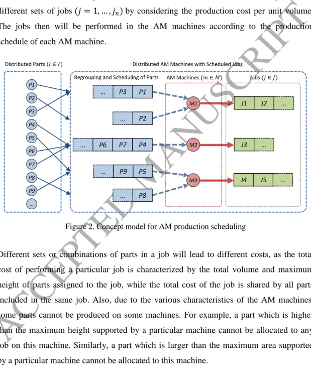
As described in Section 1, this paper studies production planning of distributed AM machines to fulfill demands received from individual customers in low quantities. The production with powder-bed based AM machines is operated on a job by job basis. The capacity of a given AM machine depends on its total available production area and allowed maximum part height. Each AM machine will be assigned a relatively fixed labor cost and time cost, and a particular process parameter will be set with a specified building speed and layer thickness. The distributed fabrication orders will be dispersed on a part by part basis using specific height, production area, and material volume. The problem is how to regroup the given parts from distributed customers and allocate them to distributed AM machines with various cost and speed characteristics by minimizing average production cost per unit volume of material. The concept model is depicted in Figure 2.
ACCEPTED MANUSCRIPT
As seen from Figure 2, the problem consists of a set of AM machines , where each AM machine has different specifications, including operation cost, production efficiency and maximum supported area and height. There exists a set of parts with different volumes, heights and production areas as determined by the customer’s demands. The parts will be allocated to AM machines and then grouped as different sets of jobs by considering the production cost per unit volume. The jobs then will be performed in the AM machines according to the production schedule of each AM machine.
Figure 2. Concept model for AM production scheduling
Different sets or combinations of parts in a job will lead to different costs, as the total cost of performing a particular job is characterized by the total volume and maximum height of parts assigned to the job, while the total cost of the job is shared by all parts included in the same job. Also, due to the various characteristics of the AM machines, some parts cannot be produced on some machines. For example, a part which is higher than the maximum height supported by a particular machine cannot be allocated to any job on this machine. Similarly, a part which is larger than the maximum area supported by a particular machine cannot be allocated to this machine.
Distributed Parts 𝑖 ∈ 𝐼 P2 P3 P4 P8 P9 M1 P1 M2 M3 J2 …
Regrouping and Scheduling of Parts
Distributed AM Machines with Scheduled Jobs
P1 P3 … P2 P7 P6 … P5 P6 P7 P5 J5 … P8 AM Machines 𝑚 ∈ 𝑀 … … P9 Jobs 𝑗 ∈ 𝐽 J3 J4 J1 … P4 … …
ACCEPTED MANUSCRIPT
2.1. Assumptions
The production area of parts considered in this study is not the real production area. To obtain production area of a part, some tolerance was added to its real area, which provides us flexibility in allocating parts on to the platform of the AM machine without having to consider a sophisticated nesting problem. Each part has a predefined orientation according to the quality and the requirements of the additive manufacturing process. Therefore, parts can only be moved on the platform horizontally while it is not allowed to rotate the parts vertically. As this study is the first of its kind, only one type of material is considered in this study to keep the complexity of the model at a minimum and focus on the main idea underlying the research. Additionally, no due dates are taken into account for fulfilling orders for the same reason.
2.2. Mathematical model 2.2.1. Notation
The following notations are used in the formulation of the mathematical model of the problem:
part index and job index ; and machine index and height of part
production area of part material volume of part
cost per unit volume of material
operation cost per unit time for machine
time for forming per unit volume of material for machine accumulated interval time per unit height for machine
cost of human work per time unit (will be used to calculate set-up cost)
set-up time needed for machine
maximum height of part that machine can process
maximum production area of part that machine can process production cost of job on machine
ACCEPTED MANUSCRIPT
2.2.2. Decision variables
{
{ 2.2.3. Objective function
In terms of the notation given above, the production cost of job on machine , represented by , can be formulated as follows:
∑
∈
∈ { } where is the set of parts assigned to job on machine ∈ .
The production cost of an AM job is comprised of three sections: cost of material melting depending on the material volume of parts; cost of powder layering depending on the maximum height of parts in the same job; and cost of setting up a new job. The cost of setting up a new job and powder layering are shared by all parts within the same job. There is no cost for changing the material as it is assumed that only one type of material is used for all machines.
The ultimate goal of the proposed model in this study is to minimize the average production cost per volume of material for the whole system (including all jobs on all machines). Therefore, the objective function is formulated as follows:
∑ ∑∑
∈ 2.2.4. Constraints
Part Occurrence/Assignment Constraint:
Parts cannot be split into more than one job. Therefore, each part must be allocated to one job exactly.
∑
ACCEPTED MANUSCRIPT
Job Occurrence Constraint:
Each planned job can be assigned to one machine only when there is at least one part assigned in this job. In other words, if any part is assigned to job , must be assigned to exactly one machine.
∑
∈ where is an indicator variable, { ∑ ∈
.
Capacity Constraint:
The total area needed to produce parts assigned to each job on each machine must be smaller than the available area of that machine.
∑ ∈
∈ ∈ The maximum height of parts assigned to a job on a specific machine cannot exceed the maximum height supported by this particular machine.
∈ { } ∈ ∈ Job Utilization Constraint:
Jobs will be utilized incrementally, starting from the first job ( , and so on). In other words, a new job can be utilized by a machine if all of its previous jobs have been utilized.
∈ { } ∈ { } ∈ where is the set of parts assigned to job .
3. Heuristic Procedures (BF and ABF)
The mathematical model is presented in the previous section for the production planning problem of AM machines. However, pre-emptive experiments have shown that it is not possible to get optimal solutions in reasonable CPU times when the problem size increases. For that reason, we also propose two heuristic rules, namely best-fit (BF) and adapted best-fit (ABF), for solving the problem efficiently. This section explains the solution-building mechanism of both algorithms step-by-step.
ACCEPTED MANUSCRIPT
3.1. Heuristic regrouping and scheduling procedure
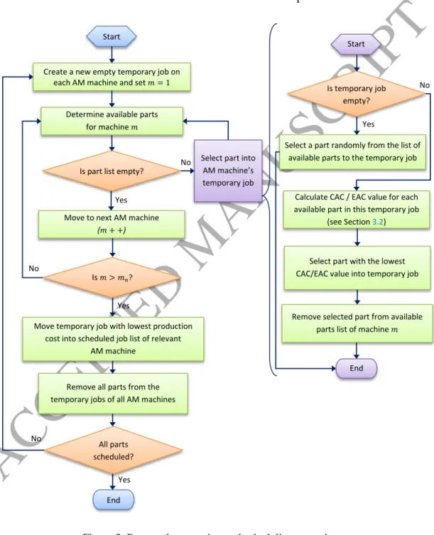
Both heuristic procedures, namely BF and ABF, use the same regrouping and scheduling procedure given in Figure 3. The difference between BF and ABF is the decision rule that is applied to select parts from the list of available parts. This rule determines which part to select based on the calculated cost structures that will be explained in Section 3.2.
Figure 3. Proposed regrouping and scheduling procedure Create a new empty temporary job on
each AM machine and set 𝑚
End Is part list empty?
Start
Select part into AM machine’s temporary job
Is 𝑚 > 𝑚𝑛?
Move to next AM machine
(𝑚 )
Move temporary job with lowest production cost into scheduled job list of relevant
AM machine
Remove all parts from the temporary jobs of all AM machines
Start
Select a part randomly from the list of available parts to the temporary job
Is temporary job empty?
Calculate CAC / EAC value for each available part in this temporary job
(see Section 3.2)
Select part with the lowest CAC/EAC value into temporary job
End No Yes Yes No No
Determine available parts for machine 𝑚 Yes No Yes All parts scheduled?
Remove selected part from available parts list of machine 𝑚
ACCEPTED MANUSCRIPT
To clearly explain this procedure, it is important to define the terms job, temporary job, assigned part and scheduled part. Each AM machine keeps a temporary job to regroup given parts and allocate them to jobs. A temporary job is called a job if it is scheduled on an AM machine. An assigned part is a part which has been assigned to a temporary job. On the other hand, a scheduled part means a part which is assigned to a job which is eventually scheduled on a machine. This means that part cannot be assigned to any other job or temporary job.
As seen in Figure 3, the procedure starts with creating a new empty temporary job on each AM machine. Available parts are determined for the first machine considering its specifications, i.e. the remaining area on the platform and the maximum height supported. Available parts for a machine are determined from those which have neither been scheduled previously nor assigned to this machine’s temporary job. Among the available ones, parts are selected one-by-one and allocated to the temporary job. If this is the first part (i.e. the temporary job is empty), it is selected randomly to get diversified solutions. This is why the selection of the first part affects the selection of the remaining ones due to the cost models (which will be given in the following subsections) and helps the algorithm scan the search space more effectively. Otherwise, as the algorithm employs a constructive single-pass mechanism, the same solution would be produced every time it was run. The list of available parts is updated every time a new part is selected to a temporary job. Thus, the part assigned to the temporary job on this machine is removed from its available parts list. The subsequent parts (i.e. the second, the third and so on) are selected based on their CAC/EAC values (of which the calculations will be explained in Section 3.2) and this cycle continues until there is no part available for this temporary job on the first machine. The algorithm moves to the next machine ( ++) and the available parts are determined for this machine. To remind, the parts which have been assigned to the temporary job on the previous machine can be available for this machine since those parts have not been scheduled yet. At this stage, a part can be assigned to more than one temporary job on different machines (not the same machine). The first part and the subsequent ones are selected to this machine (until there is no available part) as in the first machine and a temporary job is obtained for this machine as well.
ACCEPTED MANUSCRIPT
The algorithm moves to the next machine ( ++) and eventually, a temporary job is constructed on all AM machines in this way. The production cost of each temporary job is calculated using Equation (1) given in Section 2.2.3 and the one which has the lowest production cost is converted to a scheduled job on the corresponding AM machine (e.g. if the temporary job of machine 2 has the lowest, it is scheduled on machine 2). The parts existing in a scheduled job cannot be available for any other temporary job any more as they have already been scheduled permanently. Thus, it is ensured that each part is assigned to exactly one machine. New temporary jobs are created on all AM machines. Starting from the first machine, available parts are determined and assigned to temporary jobs following the same procedure used in the previous cycle until the remaining capacity is not enough to accommodate any more parts. The temporary job which has the lowest production cost is scheduled and this cycle continues until there is no part unscheduled. The objective function value of the solution is calculated using Equation (2) given in Section 2.2.3. The algorithm is run repeatedly until the maximum number of iterations is exceeded and the best solution which gives the minimum objective function value is taken.
3.2. Calculation of cost structures
In order to get solutions with two heuristic algorithms proposed, two different cost structures are adopted to decide which part to assign to temporary jobs on the machines. For the BF heuristic algorithm, when part ∈ is subject to selection, the value of the current average cost per unit volume of material ( ) for a temporary job on machine ∈ is calculated as follows:
∑ ∈
∈ { }
∑ ∈
where is the collection of parts which have been assigned to the temporary job of machine so far (including candidate part ). This value will be equal to when there is no part assigned to the same job before part . is calculated for all available parts and the part which has the lowest is assigned to the temporary job of AM machine ∈ .
ACCEPTED MANUSCRIPT
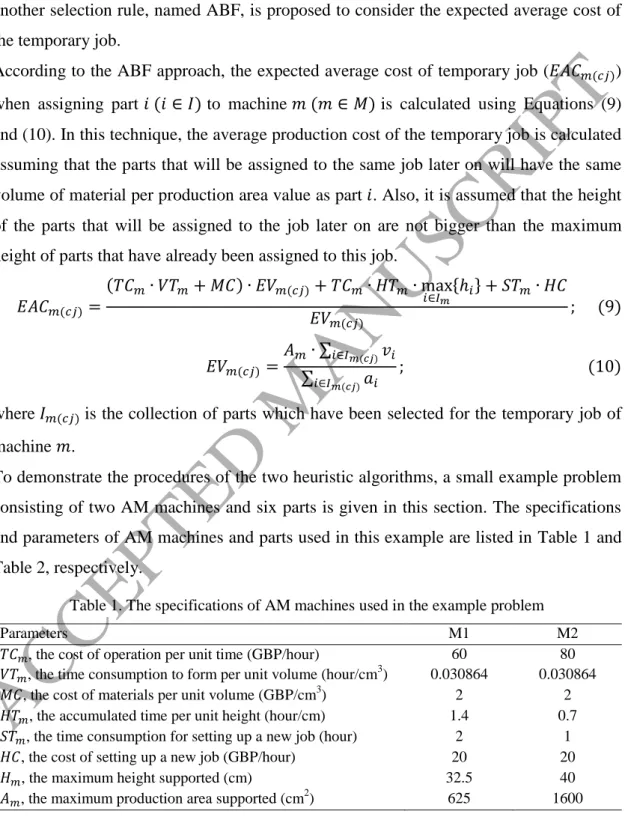
In this approach, the part with the shortest height and the largest volume will most likely be assigned to a temporary job. This policy can result in missing some better combinations of parts, which may lead to less efficient production costs. Therefore, another selection rule, named ABF, is proposed to consider the expected average cost of the temporary job.
According to the ABF approach, the expected average cost of temporary job ( ) when assigning part ∈ to machine ∈ is calculated using Equations (9) and (10). In this technique, the average production cost of the temporary job is calculated assuming that the parts that will be assigned to the same job later on will have the same volume of material per production area value as part . Also, it is assumed that the height of the parts that will be assigned to the job later on are not bigger than the maximum height of parts that have already been assigned to this job.
∈ { } ∑ ∈ ∑ ∈ where is the collection of parts which have been selected for the temporary job of machine .
To demonstrate the procedures of the two heuristic algorithms, a small example problem consisting of two AM machines and six parts is given in this section. The specifications and parameters of AM machines and parts used in this example are listed in Table 1 and Table 2, respectively.
Table 1. The specifications of AM machines used in the example problem
Parameters M1 M2
, the cost of operation per unit time (GBP/hour) 60 80 , the time consumption to form per unit volume (hour/cm3) 0.030864 0.030864 , the cost of materials per unit volume (GBP/cm3) 2 2 , the accumulated time per unit height (hour/cm) 1.4 0.7 , the time consumption for setting up a new job (hour) 2 1 , the cost of setting up a new job (GBP/hour) 20 20
, the maximum height supported (cm) 32.5 40 , the maximum production area supported (cm2) 625 1600
ACCEPTED MANUSCRIPT
Table 2. The specifications of parts used in the example problem
Part () Height ( ) in cm Volume ( ) in cm3 Production Area ( ) cm2
P1 25.10 2867.59 569.53 P2 37.25 2378.05 464.89 P3 39.24 16420.91 779.96 P4 4.27 102.83 122.62 P5 13.56 3640.48 390.39 P6 2.18 214.79 178.34
Table 3 and Table 4 show the part selection procedure steps for BF and ABF procedures, respectively. As mentioned previously, both heuristics use the same procedure to build an assignment solution. The only difference between the two approaches is the part selection rule, which is characterized by the average cost calculation principle. and values of temporary jobs are calculated using Equations (8) - (10) introduced in Section 3.2.
Table 3. Part selection procedure based on CAC values (BF rule)
Step Machine
The CAC value of available parts for temporary
job Min. CAC
(GBP/cm3) Part(s) in the temporary job Scheduled job(s) P1 P2 P3 P4 P5 P6
1 M1 4.601 N/A N/A 7.729 4.176 4.891 4.601 P1 N/A
M2 5.355 4.754 4.604 6.989 4.683 5.131 4.604 P3 N/A 2 M1 N/A N/A N/A N/A N/A N/A 4.601 P1 N/A M2 4.584 4.587 N/A 4.603 4.58 4.602 4.58 P3,P5 N/A 3 M1 N/A N/A N/A N/A N/A N/A 4.601 P1 N/A M2 N/A N/A N/A 4.579 N/A 4.578 4.578 P3,P5,P6 N/A 4 M1 N/A N/A N/A N/A N/A N/A 4.036 P1 N/A
M2 N/A N/A N/A 4.578 N/A N/A 4.578 P3,P5,P6,P4 N/A
5 M1 N/A N/A N/A N/A N/A N/A 4.036 P1 [P1]
M2 N/A N/A N/A N/A N/A N/A 4.578 P3,P5,P6,P4 N/A 6 M1 SC N/A N/A 7.729 4.176 4.891 4.176 P5 [P1] M2 SC N/A N/A N/A N/A N/A 4.578 P3,P5,P6,P4 N/A 7 M1 SC N/A N/A 4.167 N/A 4.158 4.158 P5,P6 [P1] M2 SC N/A N/A N/A N/A N/A 4.578 P3,P5,P6,P4 N/A
8 M1 SC N/A N/A N/A N/A N/A 4.158 P5,P6 [P1],[P5,P6]
M2 SC N/A N/A N/A N/A N/A 4.578 P3,P5,P6,P4 N/A
9 M1 SC N/A N/A 7.729 SC SC 7.729 P4 [P1],[P5,P6]
M2 SC 4.586 N/A N/A SC SC 4.586 P3,P4,P2 N/A
10 M1 SC N/A N/A N/A SC SC 7.729 P4 [P1],[P5,P6]
M2 SC N/A N/A N/A SC SC 4.586 P3,P4,P2 [P3,P4,P2]
11 M1 SC SC SC SC SC SC N/A N/A [P1],[P5,P6] M2 SC SC SC SC SC SC N/A N/A [P3,P4,P2]
ACCEPTED MANUSCRIPT
* Please note that SC denotes that the job has already been scheduled.In the first step, randomly selected parts are assigned to the temporary jobs of the machines. In our example, the assigned parts are P1 and P3 for M1 and M2 (respectively) for the BF heuristic (see Step 1 in Table 3), while P5 is selected on both machines for the ABF rule (see Step 1 in Table 4). In Step 2, the availability of each part for each machine is updated based on its production area, height, and the machine’s available production area and supported height. Also, the CAC (or EAC) values of the temporary jobs are calculated for all available parts to see what the average production cost will be if a particular part is assigned to this job. The parts which give the minimum CAC (or EAC) value are assigned to the temporary jobs of M1 and M2.
Table 4. Part selection procedure based on EAC values (ABF rule)
Step Machine
The EAC value of available parts for
temporary job Min. EAC (GBP/cm3)
Part(s) in the
temporary job Scheduled job(s) P1 P2 P3 P4 P5 P6
1 M1 4.535 N/A N/A 4.612 4.054 4.148 4.054 P5 N/A M2 4.646 4.726 4.535 4.662 4.521 4.543 4.521 P5 N/A
2 M1 N/A N/A N/A 4.11 N/A 4.13 4.11 P5,P4 N/A
M2 4.601 4.656 4.55 4.536 N/A 4.541 4.536 P5,P4 N/A 3 M1 N/A N/A N/A N/A N/A N/A 4.11 P5,P4 N/A M2 4.615 4.679 4.558 N/A N/A 4.554 4.554 P5,P4,P6 N/A 4 M1 N/A N/A N/A N/A N/A N/A 4.11 P5,P4 N/A M2 4.634 4.709 4.569 N/A N/A N/A 4.569 P5,P4,P6,P3 N/A
5 M1 N/A N/A N/A N/A N/A N/A 4.11 P5,P4 [P5,P4]
M2 N/A N/A N/A N/A N/A N/A 4.569 P5,P4,P6,P3 N/A 6 M1 4.535 N/A N/A SC SC 4.148 4.148 P6 [P5,P4]
M2 4.578 4.573 N/A SC SC N/A 4.573 P6,P3,P2 N/A
7 M1 N/A N/A N/A SC SC N/A 4.148 P6 [P5,P4],[P6]
M2 N/A N/A N/A SC SC N/A 4.573 P6,P3,P2 N/A
8 M1 4.535 N/A N/A SC SC SC 4.535 P1 [P5,P4],[P6]
M2 N/A N/A N/A SC SC SC 4.584 P3,P2 N/A
9 M1 N/A N/A N/A SC SC SC 4.535 P1 [P5,P4],[P6],[P1]
M2 N/A N/A N/A SC SC SC 4.584 P3,P2 N/A
10 M1 SC N/A N/A SC SC SC N/A N/A [P5,P4],[P6],[P1]
M2 SC N/A N/A SC SC SC 4.584 P3,P2 [P3,P2]
11 M1 SC SC SC SC SC SC N/A N/A [P5,P4],[P6],[P1] M2 SC SC SC SC SC SC N/A N/A [P3,P2]
Average Production Cost: 4.5298 GBP/cm3
For the BF heuristic, P5 is assigned to the temporary job of M2, while there is no available part for M1. For the ABF rule, P4 is assigned to the temporary jobs of both M1 and M2, simultaneously. This cycle repeats until there are no available parts for any of the machines (i.e. see Step 5 for both BF and ABF procedures). Afterwards, the CAC (or
ACCEPTED MANUSCRIPT
EAC) values of the temporary jobs on M1 and M2 are compared. The job which has the minimum CAC (or EAC) value is assigned to the relevant machine’s scheduled job list (which is now considered a permanent job). In our case, the temporary job on M1 is assigned to the scheduled jobs list for both BF and ABF heuristic procedures. The scheduled job in BF has only one part, i.e. P1, while it contains P5 and P4 in ABF. Therefore, in the ABF heuristic, P5 and P4 are removed from the temporary job of M2 (see Step 5 and Step 6 in Table 4). For the BF heuristic, there is no need to remove P1 from any list at this stage, as P1 is not in the temporary list of M2 (see Step 5 in Table 3). After that, the scheduled parts are removed from all temporary jobs on all machines and marked as assigned. The available parts are determined again and the ones which provide the minimum average production costs are assigned to temporary jobs. This cycle continues until all parts are scheduled on exactly one AM machine. For the BF rule, the final solution is that jobs [P1] and [P5, P6] are scheduled on M1, and job [P3, P4 and P2] is scheduled on M2, which provides an average production cost of 4.5236 GBP/cm3. For ABF, the final scheduled jobs are [P5, P4], [P6] and [P1] on M1 and [P3, P2] on M2, with an average production cost of 4.5298 GBP/cm3.
4. Numerical Example
4.1. Problem data
A numerical example is given in this section to describe the AM machines’ planning problem and to demonstrate the optimal solution of an example problem, along with the heuristic solutions proposed for comparison purposes. The optimal solution of the problem is obtained through developing the mathematical model presented in Section 2.2 on IBM CPLEX Optimization Studio 12.6.1.
A small example problem consisting of 2 AM machines (M1 and M2) with different specifications and 10 parts (P1-P10), with random heights, volumes and production areas, was created. The parameters related to the AM machines are determined based on the authors’ experiences in operations of SLM equipment. The related specifications and parameters of AM machines are listed in Table 5. The height, volume, and production area of each part are generated randomly within the range allowed by the AM machines and presented in Table 6.
ACCEPTED MANUSCRIPT
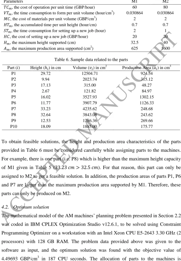
Table 5. The specifications and parameters of the AM machines
Parameters M1 M2
, the cost of operation per unit time (GBP/hour) 60 80 , the time consumption to form per unit volume (hour/cm3) 0.030864 0.030864 , the cost of materials per unit volume (GBP/cm3) 2 2 , the accumulated time per unit height (hour/cm) 0.7 0.7 , the time consumption for setting up a new job (hour) 2 1 , the cost of setting up a new job (GBP/hour) 20 20
, the maximum height supported (cm) 32.5 40 , the maximum production area supported (cm2) 625 1600
Table 6. Sample data related to the parts
Part () Height ( ) in cm Volume ( ) in cm2 Production Area ( ) in cm3
P1 29.72 12504.71 924.34 P2 9.94 2023.74 315.12 P3 17.13 315.00 48.27 P4 2.67 121.82 84.97 P5 16.02 3527.93 1302.15 P6 11.77 3907.79 1126.33 P7 33.23 4235.62 248.68 P8 32.64 3843.08 243.62 P9 12.53 1786.36 269.66 P10 18.09 1885.00 175.77
To obtain feasible solutions, the height and production area characteristics of the parts provided in Table 6 must be considered carefully while assigning parts to the machines. For example, there is one part (i.e. P8) which is higher than the maximum height capacity of M1 given in Table 5 ( > ). For that reason, this part can only be assigned to M2 to get a feasible solution. In addition, the production areas of parts P1, P6 and P7 are larger than the maximum production area supported by M1. Therefore, these parts can only be produced on M2.
4.2. Optimum solution
The mathematical model of the AM machines’ planning problem presented in Section 2.2 was coded in IBM CPLEX Optimization Studio v12.6.1, to be solved using Constraint Programming Optimizer on a workstation with an Intel Xeon CPU E5-2643 3.30 GHz (2 processors) with 128 GB RAM. The problem data provided above was given to the software as input, and the optimum solution was found with the objective value of 4.49693 GBP/cm3 in 187 CPU seconds. The allocation of parts to the machines is
ACCEPTED MANUSCRIPT
presented in Table 7. Please note that the upper limit for the total number of jobs ( ) was calculated as ⌈ ⌉ , rather than , where is the total number of parts and ⌈ ⌉ denotes the smallest integer which is equal to or greater than . This action was taken to narrow the solution space and get the optimum solution in a shorter time.
Table 7. The optimum allocation of ten parts
Machine Job Scheduled Parts Max Height (cm) Total Production Area (cm2)
M1 J4 P2, P4 9.94 400.09
M1 J5 P3, P9, P10 18.09 493.70
M2 J1 P1, P7, P8 33.23 1416.64
M2 J2 P5 16.02 1302.15
M2 J3 P6 11.77 1126.33
As can be seen from Table 7, a total of five jobs were utilized to produce ten parts. For example, Job 4 was scheduled to produce parts P2 and P4 on M1, where the maximum height of the parts is 9.94 cm, and the total production area requirement for this job is 400.09 cm2. As it can be seen, the maximum height and total production area of the parts do not exceed the supported specifics of M1 ( and ). Similarly, P1, P7 and P8 were assigned to J1, which is scheduled to be performed on M2. The maximum height of the parts assigned to this job is 33.23 cm, while the total production area of the parts is 1416.64 cm2, both of which are supported by M2. Figure 4 shows the maximum heights and total areas of the utilized jobs in comparison to the specifics of the machines.
Figure 4. Maximum heights and total areas of the utilized jobs, J1-J3 on M2 and J4-J5 on M1
0 5 10 15 20 25 30 35 40 1 2 3 4 5 M axi m u m Hei gh t (c m ) Job Number
H1 Zone H2 Zone max_hi (cm)
0 200 400 600 800 1000 1200 1400 1600 1 2 3 4 5 To tal A re a ( cm 2) Job Number
ACCEPTED MANUSCRIPT
4.3. Heuristic solutions
To give an insight into the performance of the proposed heuristics, namely BF and ABF, we solved the same numerical example problem using both of the heuristic procedures. BF and ABF were run for 25 iterations on the same workstation with CPLEX, for which the specifications were given in the previous subsection, and the best solutions are reported in Table 8.
The objective function values of the solutions (which are calculated using Equations (1) and (2)) are also presented in Table 8, along with the CPU time consumed. Convergence of the BF and ABF procedures throughout 25 iterations is also depicted in Figure 5 and Figure 6, respectively. When the solutions obtained by BF and ABF are compared to the solution obtained by CPLEX, it is clear that the solution found by ABF is optimal.
Table 8. The best solutions obtained by BF and ABF procedures
Machine Job Scheduled Parts
Max Height (cm) Total Area Needed (cm2) Objective Function Value (GBP/cm3) CPU Time (seconds) BF M1 J1 P2, P9 12.53 584.78 4.50012 9.957 M1 J2 P4, P10, P3 18.09 309.01 M2 J3 P1, P7, P8 33.23 1416.64 M2 J4 P5 16.02 1302.15 M2 J5 P6 11.77 1126.33 AB F M1 J1 P3, P10, P9, P4 18.09 578.67 4.49693 10.979 M1 J2 P2 9.94 315.12 M2 J3 P7, P8, P1 33.23 1416.64 M2 J4 P5 16.02 1302.15 M2 J5 P6 11.77 1126.33
Figure 5. The convergence of BF procedure
4.49 4.50 4.51 4.52 4.53 4.54 4.55 4.56 1 2 3 4 5 6 7 8 9 10 11 12 13 14 15 16 17 18 19 20 21 22 23 24 25 OBJ Valu e (G BP/cm 3) Iteration Number CAC_OBJ
ACCEPTED MANUSCRIPT
Figure 6. The convergence of ABF procedure
5. Computational Study
This section provides comprehensive experimental test results obtained through (i) the proposed mathematical model coded in IBM CPLEX Optimization Studio v12.6.1; and (ii) the proposed BF and ABF heuristics coded in JavaScript. Constraint Programming Optimizer was used in CPLEX to get solutions on a workstation with the specifications of Intel Xeon CPU E5-2643 3.30GHz (2 processors) with 128 GB RAM. The BF and ABF heuristics were also run on the same workstation for the accuracy of the comparisons that will be made.
5.1. Test data
Table 9 presents the data generated based on some preliminary work and the authors’ experience in the AM industry. A master dataset (which can be accessed permanently at the University of Exeter’s ORE-Repository [18]) consisting of large lists of parts and machines was created. To build test problems, the parts and machines were selected from these lists with some rules given in Table 9. In the table, the Range of Parts and Range of Machines columns determine which parts and machines are considered in each test problem (the specific test problems are also available online at the website given above). These ranges are determined systematically to provide a diversified set of test problems in various problem sizes.
5.2. Test results
Table 10 reports computational test results obtained through solving the aforementioned test problems using the CPLEX software and the BF and ABF heuristics. The NJ and
4.49 4.51 4.53 4.55 1 2 3 4 5 6 7 8 9 10 11 12 13 14 15 16 17 18 19 20 21 22 23 24 25 OBJ Valu e (G BP/cm 3) Iteration Number EAC_OBJ
ACCEPTED MANUSCRIPT
Table 9. Data for computational tests
# Number of Parts
Number of Machines
Range of Parts Range of Machines
Begins (including) Ends (including) Begins (including) Ends (including) 1 10 2 1 10 1 2 2 12 2 11 22 2 3 3 14 2 23 36 4 5 4 16 2 37 52 5 6 5 18 2 53 70 7 8 6 20 2 71 90 8 9 7 15 3 91 105 1 3 8 18 3 106 123 2 4 9 21 3 124 144 3 5 10 24 3 145 168 4 6 11 27 3 169 195 5 7 12 30 3 196 225 6 8 13 20 4 226 245 1 4 14 24 4 246 269 2 5 15 28 4 270 297 3 6 16 32 4 298 329 4 7 17 36 4 330 365 5 8 18 40 4 366 405 6 9 19 25 5 406 430 10 14 20 30 5 431 460 11 15 21 35 5 461 495 12 16 22 40 5 496 535 13 17 23 60 5 536 595 14 18 24 80 5 596 675 15 19 25 100 5 676 775 16 20 26 120 5 776 895 17 21 27 140 5 1 140 18 22 28 160 5 141 300 19 23 29 180 5 301 480 20 24 30 200 5 481 680 21 25 31 30 6 681 710 20 25 32 60 6 711 770 21 26 33 90 6 771 860 22 27 34 120 6 861 980 23 28 35 160 6 1 160 24 29 36 200 6 161 360 25 30 37 250 6 361 610 26 31 38 300 6 611 910 27 32 39 360 6 1 360 28 33 40 420 6 361 780 29 34 41 590 6 1 590 30 35 42 660 6 1 660 31 36
ACCEPTED MANUSCRIPT
OBJ columns report the number of jobs and objective function values (calculated using Equations (1) and (2)) belonging to the solution obtained through different approaches for each test problem. For each test problem, an upper limit was determined for the number of jobs for the CPLEX program (see the NJU column in Table 10) based on the solutions obtained from the heuristic algorithms. Thus, this limit did not cause infeasibility but provided some slackness.
CPLEX results were obtained through three different ways under the predetermined upper limit for the number of jobs in order to reduce computation time. First, all problems were attempted to be solved with no CPU time limit, which means the solutions obtained from this approach are optimal. However, the optimum results were only obtained for the first two test problems, #1 and #2, due to the increasing complexity of the problems and out of memory errors for the remaining test problems. This error is caused by the exponentially increasing search space with the increasing problem size. The CPU column shows the processor time consumed to get the optimum solution for these two problems. Second, the algorithm was run with a 2,000 second CPU time limit for problems #1–#18 and a 4,000 second CPU time limit for the remaining problems (see the 2K/4K CPU Limit column). Finally, the CPU time limit was increased to 4,000 seconds for test problems #1–#18 and 8,000 seconds for the remaining test problems (see the 4K/8K CPU Limit column). Due to the exponentially increasing search space with the increasing number of parts, number of jobs and number of machines, the solutions were only obtained for test problems #1–#26, #28, #31–#36.
Heuristic results were obtained using the BF and ABF procedures explained in Section 3. The maximum number of iterations for both heuristics has been set to 50, 100 and 150 for test problems #1–#9, #10–#22, and #23–#42, respectively. These numbers have been determined after a set of preliminary tests with consideration of the problem complexity, which is affected by the number of machines and the number of parts. The best solutions found for each test problem are presented in Table 10. The IT column gives the number of iterations in which the best solution was found by each heuristic, while the D% column denotes the deviation of the obtained heuristic results from the best CPLEX result (CPLEX 4K/8K CPU Limit) in terms of the OBJ value. For example, D% is calculated for a BF result as follows: ⁄ .
ACCEPTED MANUSCRIPT
Table 10. Computational test results
Test Problem # CPLEX Simple Ordered Schedule Proposed Heuristics NJU No CPU Limit 2K/4K CPU Limit 4K/8K
CPU Limit BF ABF
NJ OBJ CPU NJ OBJ NJ OBJ NJ OBJ IT NJ OBJ CPU D% IT NJ OBJ CPU D%
1 6 5 4.49693 178.77 5 4.49693 5 4.49693 5 4.5001 14 5 4.50011 28.7 0.07 6 5 4.49693 16.9 0 2 5 4 4.55895 514.50 4 4.55895 4 4.55895 5 5.1178 15 4 4.56109 27.1 0.05 17 4 4.55895 18.0 0 3 8 - - - 7 7.53692 7 7.53692 6 7.9054 3 7 7.53692 43.1 0.00 7 7 7.54115 22.7 0.06 4 11 - - - 10 7.40305 10 7.40305 8 7.7738 21 10 7.40305 46.3 0.00 20 10 7.40870 27.8 0.08 5 11 - - - 10 7.45879 10 7.45879 7 7.7302 24 10 7.46019 53.2 0.02 5 10 7.46136 34.0 0.03 6 10 - - - 9 7.83539 9 7.83539 7 8.1314 10 9 7.83876 49.4 0.04 27 9 7.84619 26.3 0.14 7 10 - - - 8 4.49170 8 4.49170 8 4.7657 32 9 4.49833 46.1 0.15 11 9 4.49134 25.3 -0.01 8 7 - - - 6 4.58228 6 4.58228 9 5.1330 24 6 4.59050 52.2 0.18 1 6 4.59425 30.8 0.26 9 10 - - - 8 8.03319 8 8.03319 8 8.1235 3 8 8.05533 63.0 0.28 35 9 8.05872 35.1 0.32 10 12 - - - 10 7.33424 10 7.33424 9 7.9065 49 10 7.33424 222.1 0.00 58 11 7.34334 100.5 0.12 11 14 - - - 13 7.41312 13 7.41282 13 7.8033 41 13 7.41756 237.6 0.06 45 13 7.41487 108.5 0.03 12 20 - - - 19 7.13833 18 7.13651 15 7.6280 35 17 7.13536 297.8 -0.02 55 18 7.13857 112.5 0.03 13 12 - - - 11 4.43870 11 4.43870 10 4.8500 9 11 4.43870 223.6 0.00 10 11 4.43884 75.3 0.00 14 10 - - - 9 4.56567 8 4.56037 12 5.7389 17 8 4.56944 252.9 0.20 22 8 4.56407 90.0 0.08 15 15 - - - 14 6.80570 14 6.80570 15 7.3532 65 14 6.81087 305.1 0.08 13 14 6.80984 109.2 0.06 16 18 - - - 17 6.99616 17 6.99391 16 7.7399 10 16 6.99770 356.8 0.05 62 16 6.99562 131.6 0.02 17 23 - - - 22 6.98648 20 6.98077 17 7.7449 14 20 6.99597 400.4 0.22 68 19 6.98448 151.7 0.05 18 23 - - - 22 7.15691 21 7.14684 16 7.5355 38 17 7.15254 386.4 0.08 1 17 7.14994 159.6 0.04 19 16 - - - 15 7.51924 15 7.51924 15 7.9742 17 15 7.52013 311.6 0.01 37 15 7.52028 105.8 0.01 20 16 - - - 15 4.35269 15 4.35269 15 6.6770 26 15 4.35792 320.3 0.12 76 15 4.35716 130.1 0.10 21 20 - - - 18 4.50271 18 4.50271 18 4.8180 27 19 4.50599 428.5 0.07 84 19 4.50752 159.8 0.11 22 21 - - - 20 4.42343 20 4.42343 19 6.1940 1 20 4.42812 522.8 0.11 57 19 4.43141 205.1 0.18 23 19 - - - 18 4.57636 17 4.57057 25 6.3751 65 17 4.57788 1262.8 0.16 66 17 4.57484 466.7 0.09 24 27 - - - 26 4.59383 26 4.58640 32 7.0956 43 24 4.58343 1930.9 -0.06 94 25 4.58553 768.3 -0.02 25 49 - - - 47 7.90519 47 7.85915 35 7.9661 62 47 7.72662 3080.3 -1.69 20 48 7.72662 1165.7 -1.69
ACCEPTED MANUSCRIPT
Table 10 (continued) Test Problem # CPLEX Simple Ordered Schedule Proposed Heuristics NJU No CPU Limit 2K/4K CPU Limit 4K/8KCPU Limit BF ABF
NJ OBJ CPU NJ OBJ NJ OBJ NJ OBJ IT NJ OBJ CPU D% IT NJ OBJ CPU D%
26 33 - - - 32 4.60723 32 4.60229 37 7.3485 123 32 4.58813 1288.7 -0.31 115 32 4.58435 1472.6 -0.39 27 42 - - - - - 53 7.2721 87 40 4.58319 1695.3 - 14 41 4.58469 1967.8 -28 49 - - - 47 6.45456 47 6.01250 55 7.0075 28 47 4.57280 2415.0 -23.95 103 48 4.57347 2725.5 -23.93 29 57 - - - 74 6.9179 122 55 4.56859 3285.7 - 88 56 4.56967 3744.5 - 30 60 - - - 85 6.4002 56 58 4.57059 3461.4 - 86 59 4.57298 4853.0 - 31 10 - - - 9 4.57545 9 4.57478 12 6.8456 84 9 4.57792 218.1 0.07 117 9 4.58178 238.2 0.15 32 17 - - - 15 4.56568 15 4.56502 23 6.1872 101 15 4.57334 499.6 0.18 3 16 4.57243 585.6 0.16 33 24 - - - 22 4.59343 22 4.58629 33 6.8676 11 22 4.58193 946.0 -0.10 101 23 4.57538 1123.3 -0.24 34 35 - - - 34 5.26663 34 4.72352 43 7.2085 43 34 4.57596 1626.1 -3.12 40 34 4.57559 1983.4 -3.13 35 47 - - - 45 4.60161 45 4.60140 58 6.4628 69 45 4.57762 2649.2 -0.52 8 46 4.57879 3402.8 -0.49 36 63 - - - 61 7.54412 61 7.22428 69 6.7314 36 61 4.56889 5981.9 -36.76 77 62 4.56746 8666.6 -36.78 37 74 - - - 82 6.8312 23 73 4.56444 8556.5 - 52 73 4.56529 10086 - 38 84 - - - 102 7.2350 1 81 4.57128 23954 - 7 83 4.57186 28928 - 39 170 - - - 151 6.8745 61 168 4.44749 22405 - 75 169 4.44584 23322 - 40 190 - - - 182 6.2958 1 185 4.45384 27409 - 14 189 4.45143 28976 - 41 274 - - - 263 6.1052 73 265 4.45706 80287 - 43 273 4.45568 95326 - 42 305 - - - 295 4.8887 59 294 4.45524 124794 - 8 304 4.45437 138509 -*
ACCEPTED MANUSCRIPT
To compare our results with what the situation could be without utilization of systematic production planning techniques, we also provided results as if the parts were assigned to the machines based on incremental orders of part numbers. In other words, starting from part 1, parts were assigned to the machines in an incremental order starting from machine 1. When the capacity of the current job on the current machine was not enough to accommodate the next job, a new job was opened on the next machine and assignment process continued from that newly-opened job. Results obtained from that simple rule are provided in the Simple Ordered Schedule column in Table 10.
To give an insight about the enormous amounts of savings that could be made by planning AM/3DP machines using sophisticated scheduling techniques, the total costs of the solutions are also calculated and reported in Table 11. To calculate the total cost of a scheduling solution of a test problem reported in Table 10, the total volume of parts in that test problem is simply multiplied by the OBJ value reported for the same test problem. The difference between the total costs of Simple Ordered Schedule solutions and CPLEX, BF, and BFA solutions are also reported for each test problem.
5.3. Discussion
As can be seen from Table 10 and Table 11, CPLEX found the optimal solutions for the first two test problems (P1-P2) in a very short amount of time. However, with an increase in the number of parts, the number of machines and the upper limit for the number of jobs, it could not find optimal solutions beyond this point. When the results in the 2K/4K CPU Limit column are compared to the results presented in the 4K/8K CPU Limit column, it can be seen that the algorithm returns the same solutions for the first ten test problems (#1–#10). However, with the increase in problem size (starting from #11), CPLEX returns better solutions with better objective function values when the CPU time limit is increased from 2,000 seconds to 4,000 seconds (for #1–#18), and to 8,000 seconds (for #19 and thereafter). Therefore, the capability of CPLEX increases when the CPU time limit is increased (see test problems #11 and thereafter), as better solutions were obtained for a total of 17 test problems.
ACCEPTED MANUSCRIPT
Table 11. The total costs of the solutions obtained
# Total Volume CPLEX Simple Ordered Schedule Heuristic Procedures No CPU
Limit 2K/4K CPU Limit 4K/8K CPU Limit BF ABF
Total Cost Total Cost Difference Total Cost Difference Total Cost Total Cost Difference Total Cost Difference 1 34151.05 £153,574.88 £153,574.88 £108.26 £153,574.88 £108.26 £153,683.14 £153,683.48 -£0.34 £153,574.88 £108.26 2 51277.84 £233,773.11 £233,773.11 £28,656.62 £233,773.11 £28,656.62 £262,429.73 £233,882.84 £28,546.89 £233,773.11 £28,656.62 3 37716.64 - £284,267.30 £13,897.83 £284,267.30 £13,897.83 £298,165.13 £284,267.30 £13,897.83 £284,426.84 £13,738.29 4 52972.41 - £392,157.40 £19,639.52 £392,157.40 £19,639.52 £411,796.92 £392,157.40 £19,639.52 £392,456.69 £19,340.23 5 51753.09 - £386,015.43 £14,046.31 £386,015.43 £14,046.31 £400,061.74 £386,087.88 £13,973.85 £386,148.44 £13,913.30 6 97587.83 - £764,638.71 £28,886.97 £764,638.71 £28,886.97 £793,525.68 £764,967.58 £28,558.10 £765,692.66 £27,833.02 7 57286.09 - £257,311.93 £15,696.39 £257,311.93 £15,696.39 £273,008.32 £257,691.74 £15,316.58 £257,291.31 £15,717.01 8 71312.58 - £326,774.21 £39,273.26 £326,774.21 £39,273.26 £366,047.47 £327,360.40 £38,687.07 £327,627.82 £38,419.65 9 57732.10 - £463,772.93 £5,213.79 £463,772.93 £5,213.79 £468,986.71 £465,051.12 £3,935.60 £465,246.83 £3,739.89 10 84383.74 - £618,890.60 £48,289.44 £618,890.60 £48,289.44 £667,180.04 £618,890.60 £48,289.44 £619,658.49 £47,521.55 11 95146.95 - £705,335.76 £37,124.44 £705,307.21 £37,152.98 £742,460.19 £705,758.21 £36,701.98 £705,502.27 £36,957.93 12 119275.10 - £851,425.02 £58,405.44 £851,207.94 £58,622.52 £909,830.46 £851,070.78 £58,759.69 £851,453.65 £58,376.81 13 81692.75 - £362,609.61 £33,600.23 £362,609.61 £33,600.23 £396,209.84 £362,609.61 £33,600.23 £362,621.05 £33,588.79 14 92724.76 - £423,350.65 £108,787.47 £422,859.21 £109,278.91 £532,138.13 £423,700.23 £108,437.90 £423,202.30 £108,935.83 15 98740.47 - £671,998.02 £54,060.41 £671,998.02 £54,060.41 £726,058.42 £672,508.50 £53,549.92 £672,406.80 £53,651.62 16 116572.13 - £815,557.27 £86,699.36 £815,294.99 £86,961.64 £902,256.63 £815,736.79 £86,519.83 £815,494.32 £86,762.30 17 144202.89 - £1,007,470.61 £109,366.36 £1,006,647.21 £110,189.75 £1,116,836.96 £1,008,839.09 £107,997.87 £1,007,182.20 £109,654.76 18 140852.58 - £1,008,069.24 £53,325.38 £1,006,650.85 £54,743.76 £1,061,394.62 £1,007,453.71 £53,940.90 £1,007,087.50 £54,307.12 19 164243.07 - £1,234,983.06 £74,724.03 £1,234,983.06 £74,724.03 £1,309,707.09 £1,235,129.24 £74,577.85 £1,235,153.87 £74,553.21 20 111738.66 - £486,363.75 £259,715.28 £486,363.75 £259,715.28 £746,079.03 £486,948.14 £259,130.89 £486,863.22 £259,215.81 21 149708.41 - £674,093.55 £47,201.56 £674,093.55 £47,201.56 £721,295.12 £674,584.60 £46,710.52 £674,813.65 £46,481.47 22 181401.63 - £802,417.41 £321,184.28 £802,417.41 £321,184.28 £1,123,601.70 £803,268.19 £320,333.51 £803,865.00 £319,736.70 23 230665.28 - £1,055,607.36 £414,906.87 £1,054,271.81 £416,242.42 £1,470,514.23 £1,055,957.97 £414,556.25 £1,055,256.75 £415,257.48 24 264204.19 - £1,213,709.13 £660,978.12 £1,211,746.10 £662,941.15 £1,874,687.25 £1,210,961.41 £663,725.84 £1,211,516.24 £663,171.01 25 323539.32 - £2,557,639.80 £19,706.78 £2,542,744.05 £34,602.53 £2,577,346.58 £2,499,865.38 £77,481.20 £2,499,865.38 £77,481.20
ACCEPTED MANUSCRIPT
Table 11 (continued) # Total Volume CPLEX Simple Ordered Schedule Heuristic Procedures No CPULimit 2K/4K CPU Limit 4K/8K CPU Limit BF ABF
Total Cost Total Cost Difference Total Cost Difference Total Cost Total Cost Difference Total Cost Difference 26 358871,69 - £1.653.404,42 £983.764,20 £1.651.631,59 £985.537,02 £2.637.168,61 £1.646.549,97 £990.618,65 £1.645.193,43 £991.975,18 27 497812,86 - - - £3.620.144,90 £2.281.570,92 £1.338.573,98 £2.282.317,64 £1.337.827,26 28 590828,26 - £3.813.536,45 £326.692,58 £3.552.354,91 £587.874,12 £4.140.229,03 £2.701.739,47 £1.438.489,56 £2.702.135,32 £1.438.093,71 29 741890,72 - - - £5.132.325,81 £3.389.394,52 £1.742.931,29 £3.390.195,77 £1.742.130,05 30 768641,54 - - - £4.919.459,58 £3.513.145,34 £1.406.314,25 £3.514.982,39 £1.404.477,19 31 109733,88 - £502.081,88 £249.112,37 £502.008,36 £249.185,89 £751.194,25 £502.352,92 £248.841,32 £502.776,50 £248.417,75 32 193419,12 - £883.089,81 £313.632,97 £882.962,15 £313.760,63 £1.196.722,78 £884.571,40 £312.151,38 £884.395,39 £312.327,39 33 267478,42 - £1.228.643,40 £608.291,40 £1.226.733,60 £610.201,19 £1.836.934,80 £1.225.567,40 £611.367,40 £1.223.815,41 £613.119,38 34 422908,39 - £2.227.302,01 £821.233,12 £1.997.616,24 £1.050.918,89 £3.048.535,13 £1.935.211,88 £1.113.323,25 £1.935.055,40 £1.113.479,73 35 568003,38 - £2.613.730,03 £1.057.162,21 £2.613.610,75 £1.057.281,49 £3.670.892,24 £2.600.103,63 £1.070.788,61 £2.600.768,20 £1.070.124,05 36 749480,96 - £5.654.174,30 -£609.118,17 £5.414.460,31 -£369.404,18 £5.045.056,13 £3.424.296,06 £1.620.760,07 £3.423.224,31 £1.621.831,83 37 1051179,10 - - - £7.180.814,67 £4.798.043,93 £2.382.770,74 £4.798.937,43 £2.381.877,23 38 978095,92 - - - £7.076.523,98 £4.471.150,32 £2.605.373,66 £4.471.717,61 £2.604.806,37 39 1317484,30 - - - £9.057.046,10 £5.859.498,43 £3.197.547,67 £5.857.324,58 £3.199.721,52 40 1618653,10 - - - £10.190.716,12 £7.209.221,88 £2.981.494,25 £7.205.320,92 £2.985.395,20 41 2317876,70 - - - £14.151.101,01 £10.330.915,66 £3.820.185,35 £10.327.716,99 £3.823.384,02 42 2528683,50 - - - £12.361.974,78 £11.265.891,65 £1.096.083,13 £11.263.691,70 £1.098.283,08
ACCEPTED MANUSCRIPT
One could argue that the fewer number of jobs the better objective function value. However, this argument is not true, as there may exist better combinations of parts in different jobs and different machines with different specifications, which increases the area utilization. For example, in test problems #9 and #12, the ABF heuristic finds solutions with OBJ values of 8.05872 GBP/cm3 and 7.13857 GBP/cm3 with 9 jobs and 18 jobs, respectively. On the other hand, the solutions found for the same test problems by the BF heuristic have OBJ values of 8.05533 GBP/cm3 and 7.13536 GBP/cm3 with NJ values of 8 and 17 (which are less than CPLEX). A similar situation is also observed for test problem #25. The BF and ABF heuristics find the same OBJ values (7.72662 GBP/cm3) for this problem with different NJ values, i.e. 47 and 48, respectively.
For a total of 20 test problems among those solved by CPLEX, its solutions with 4K/8K CPU Limit were better than those obtained by BF (see #1, #2, #5–#9, #11, #14–#23 and #31–#32); while BF outperforms CPLEX for the majority of the large-sized instances (see #24–#26, #28, #33–#36 and #12). Tie is not broken for four problems; i.e. #3, #4, #10 and #13. ABF also outperforms CPLEX (4K/8K CPU Limit) for the same large-sized test problems as BF, in addition to P7. Negative values reported in the D% column indicate that the related heuristic method has a better solution than that of CPLEX (4K/8K CPU Limit) for the corresponding problem. As seen from the table, the most remarkable difference in favor of the heuristics is observed for #28 and #36 with ~24% and ~37%, respectively, due to the sophistication of the instances dealt with.
Although there are differences in the results obtained by BF and ABF, neither of the heuristics outperformed the other to any great extent. ABF found optimal solutions for #1 and #2, and discovered better solutions than BF for 20 test problems; while BF performed better for the remaining instances, except for #25, where both methods found the same OBJ value with different NJ values (as mentioned above).
As CPLEX found optimal solutions for #1 and #2 in both conditions that ran under 2,000 second and 4,000 second CPU time limits, it is expected that it would also find optimal or at least near-optimal solutions for most of the remaining cases. Therefore, it can be argued that although the optimal solutions are unknown, the solutions found by BF and ABF are optimal or near-optimal for the majority of the remaining test problems.