A Linear Complexity Direct Solver for H-adaptive Grids
With Point Singularities
Piotr Gurgul
Department of Computer Science, AGH University of Science and Technology, Krakow, Poland [email protected]
Abstract
In this paper we present a theoretical proof of linear computational cost and complexity for a recently developed direct solver driven by hypergraph grammar productions. The solver is specialized for computational meshes with point singularities in two and three dimensions. Linear complexity is achieved due to utilizing the special structure of such grids. We describe the algorithm and estimate the exact computational cost on an example of a two-dimensional mesh containing a single point singularity. We extend this reasoning to the three dimensional meshes.
Keywords:
1
Introduction
Direct solvers are the core part of many engineering analyses performed using the Finite Element Method [4, 5]. Since they are one of the most computationally expensive part of the process, our main objective is to deliver a solver that is by an order of magnitude faster than the existing ones in terms of both sequential and parallel execution. The finite element solution process starts with the generation of a mesh approximating the geometry of the computational problem. Next, the physical phenomena governing the problem are described using Partial Differential Equation (PDEs). In addition to this differential system, boundary and initial conditions may need to be specified to guarantee uniqueness of the solution. The resulting PDE system is discretized into a system of linear equations by using the Finite Element Method. This algebraic system is inverted using a solver algorithm. The computational complexity of the state-of-the-art multi-frontal solver [6, 7] algorithm is O(Np4+N1.5) for two dimensional problems in regular and uniform grid. N refers to the number of degrees of freedom andpis a global polynomial order of approximation, which we assume to be constant, yet arbitrary.
In this paper we present a direct solver algorithm delivering O(Np3) computational com-plexity for meshes with point singularities in two and three dimensions. The computational cost and memory usage for the direct solver estimated in this paper uses the ideas expressed by the graph grammar based solver [19] prescribing the order of elimination for grids with point
Volume 29, 2014, Pages 1090–1099
ICCS 2014. 14th International Conference on Computational Science
1090 Selection and peer-review under responsibility of the Scientific Programme Committee of ICCS 2014 c
singularities. The graph grammar formalism is utilized for modeling of mesh adaptation by means of CP-graphs [11, 12, 13, 18] or hypergraphs [17]. It can be also used for expressing the solver algorithm [16, 15] Finally, the results presented in this paper can be also extended for the idea of reutilization [14], which further generalizes a concept of a linear solver for a sequence of grids.
2
2D multi-frontal sequential solver algorithm
Problems with singularities usually require direct solvers, since they are not suitable for iterative solvers due to their numerical unstability [10]. There exist iterative solvers that converge for a certain class of variational formulations, but there are no iterative solversper se that converge for every FEM problem (as opposed to direct solvers). Moreover, even the multi-grid iterative solvers [3], more suitable for processing adaptive grids, usually still utilize a direct solver over a coarser grid. This makes the use of direct solvers absolutely necessary for designing a general purpose FEM solver. Since the matrices resulting from FEM discretization are sparse, we focus on algorithms designed for sparse matrices such as a multi-frontal solver. The multi-frontal solver introduced by Duff and Reid [6, 7] is the state-of-the-art direct solver algorithm for solving systems of linear equations, which is a generalization of the frontal solver [9] algorithm. In the multi-frontal approach, the solver generates multiple frontal matrices for all elements of the mesh. It eliminates fully assembled nodes within each frontal matrix, and merges the resulting Schur complement matrices at the parent level of the tree. The frontal matrix assembles element frontal matrices to a single frontal matrix and eliminates what is possible from the single matrix, whereas the multi-frontal solver utilizes multiple frontal matrices and thus allows to reduce the size of the matrices at parent nodes of the tree.
3
Linear complexity solver for 2D problems with point
singularities
In this section we describe briefly the idea behind solvers for problems with point singularities and what are their advantages over multi-frontal solvers like MUMPS [1, 2]. The proposed linear complexity algorithm assumes anh-refined computational mesh structure and browses the elements of the mesh level by level, from the lowest (most refined) level up to the top level. The algorithm utilizes a single frontal matrix, which size is proportional to the number of browsed degrees of freedom. There arep2degrees of freedom associated with element interiors,pdegrees of freedom associated with element edges and one degree of freedom for each element vertex. Each row of the frontal matrix is associated with one degree of freedom. The solver algorithm finds the fully assembled degrees of freedom and places them at the top of the frontal matrix. Then, these rows are eliminated by subtracting them from all the remaining rows. Intuitively, we can say that element interior degrees of freedom are fully assembled once the solver touches the element, an element edge degrees of freedom are fully assembled once the solver algorithm touches all elements adjacent to an edge, and finally element vertex degrees of freedom are fully assembled once the solver algorithm touches all elements sharing the vertex. The remaining degrees of freedom must wait until the solver algorithm browses the elements from the next level. The size of the frontal matrix is limited by the number of elements on a particular level, and this implies the linear computational cost of the solver algorithm. Moreover, the behavior of the solver described above has been prescribed by the means of hypergraphs [19] introduced
by Habel and Kreowski [8] and hypergraph grammars which were their extension proposed by ´
Slusarczyk [17] for mesh transformations.
4
Estimation of the computational cost
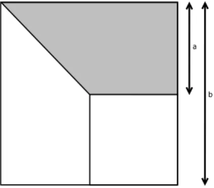
In this section we estimate the total number of operations for the 2D sequential solver described above. This will be used to obtain computational complexity. In order to compute the number of operations, we define variableaas the number of degrees of freedom that can be eliminated for matrixM andb as the total count of degrees of freedom for matrixM (see Figure 1). For
Figure 1: Visual explanation ofaandb
a given node, the total number of operations needed for its eliminationC(a, b) is equal to: C(a, b) =
b
m=b−a+1
m2 (1)
This is because we have a matrix with size b and there are a rows to be eliminated. The elimination of the first row involvesb2subtractions, the elimination of the second row involves (b−1)2subtractions, and so on, up to the last row to be eliminated, which involves (b−a+ 1)2 subtractions. Rewriting the sum in Equation 1 as a difference of two sums, we obtain Equation 2. b m=b−a+1 m2= b m=1 m2−b−a m=1 m2 (2)
which can be explicitly written using the following sum of squares: b m=1 m2=b(b+ 1)(2b+ 1) 6 (3) b−a m=1 m2= (b−a)(b−a+ 1)(2(b−a) + 1) 6 (4)
Finally, we perform the subtraction: b m=1 m2−b−a m=1 m2=a(6b2−6ab+ 6b+ 2a2−3a+ 1) 6 (5)
Thus:
C(a, b) =a(6b
2−6ab+ 6b+ 2a2−3a+ 1)
6 (6)
Using this formula, we can directly compute the costs for the sample 2D domain presented in the previous sections.
In order to prove that the computational complexity isO(N), whereN denotes the total number of unknowns, first, in Lemma 4.1, we express the exact computational cost as a function of polynomial approximation levelpand refinement levelk.
Lemma 4.1. The number of operations incurred by solving the adaptive problem with a point singularity for a two element mesh using a hypergraph grammar driven solver is equal to:
T(p, k) =16p6+ 96p5+ 264p4+ 864p3+ 533p2+ 93p 6
+k12p
6+ 72p5+ 198p4+ 1558p3−441p2−277p−24 6
where k stands for the number of h refinement levels and p is the global polynomial order of approximation. Parameterpis assumed to be uniform, yet arbitrary, over the entire mesh. Proof. With Equation 6 it is possible to evaluate the cost of each step of the elimination process. The proof can be split into two independent steps. First, we compute the constant part associ-ated with the elimination of the initial, unrefined mesh (k= 0) and then the count of operations incurred by the each increase of k by one. This is sufficient, since each layer produced as a result of incrementingkis identical and contains six new elements.
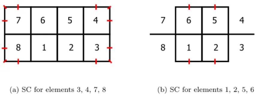
Step 1. k = 0. We begin by computing the cost of eliminating the fully assembled nodes. This process is calledstatic condensation. To eliminate entries produced by these nodes we do not need to know about any other degrees of freedom. Static condensation usually occurs just after attaching an element to the given structure. As such entries are self-contained and can be processed independently, we can count their contributions to the total number of operations independently. For each element 1, 2, 5, 6 (see Figure 2a) the interior, two edges and a vertex are fully assembled and can be eliminated immediately (or at any time). For each element 3, 4, 7, 8 (see Figure 2b) interior and only one edge are fully assembled. The number of operations
(a) SC for elements 3, 4, 7, 8
(b) SC for elements 1, 2, 5, 6
Figure 2: Static condensation fork= 0 two element mesh
sum of contributions for each of the elements in the Table 1 (which means multiplying the value in the first row by four and adding it to the value in the second row, also multiplied by four). The next step is to count the operations incurred by the interface elimination, still for
Table 1: Operations incurred by static condensation fork= 0
Elements afor arbitraryp bfor arbitraryp C(a, b)
3, 4, 7, 8 1 + 2(p−1) + (p−1)2 4 + 4(p−1) + (p−1)2 2p6+12p5+33p64+36p3+13p2 1, 2, 4, 6 p−1 + (p−1)2 4(p−1) + (p−1)2 2p6+12p5+33p46+2p3−32p2−13p TOTAL 16p6+96p5+264p46+136p3−19p2−13p
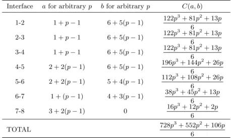
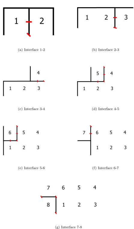
thek= 0 two element grid. This time, we need to obey the proper order for the elimination, starting from what is operationally calledInterface 1-2. In general, during this step we follow the previously described order of elimination, which is concisely summarized in Figure 3. The results are presented in Table 2. Now we have finished the first step of computations and
Table 2: Computational cost incurred by element elimination fork= 0 Interface afor arbitraryp bfor arbitraryp C(a, b)
1-2 1 +p−1 6 + 5(p−1) 122p 3+ 81p2+ 13p 6 2-3 1 +p−1 6 + 5(p−1) 122p 3+ 81p2+ 13p 6 3-4 1 +p−1 6 + 5(p−1) 122p 3+ 81p2+ 13p 6 4-5 2 + 2(p−1) 6 + 5(p−1) 196p 3+ 144p2+ 26p 6 5-6 2 + 2(p−1) 5 + 4(p−1) 112p 3+ 108p2+ 26p 6 6-7 1 + (p−1) 4 + 3(p−1) 38p 3+ 45p2+ 13p 6 7-8 3 + 2(p−1) 0 16p 3+ 12p2+ 2p 6 TOTAL 728p 3+ 552p2+ 106p 6
received the constant part fork= 0, which can be expressed asT(p,0) in Equation 7. T(p,0) = 728p
3+ 552p2+ 106p+ 16p6+ 96p5+ 264p4+ 136p3−19p2−13p
6 (7)
= 16p6+ 96p5+ 264p4+ 864p3+ 533p2+ 93p 6
Step 2. The second step of the proof is to compute the linear increase of the operation count depending onk. Increasingkby one adds one more layer of elements as presented in Figure 4. Again, for simplicity, we introduce temporary naming for the consecutive interfaces (Interface 1-2 to Interface 7-8) that will be processed (which corresponds to 3 + 6kto 8 + 6k).
Figure 4: Ordering for arbitraryk
As in Step 1, we begin with the contribution of static condensation. In the case of elements 3 + 6k and 8 + 6k we can eliminate for each one edge and its interior independently. For the remaining elements the elimination of their interiors is the only possibility at this point. The results has been summarized in Table 3. In terms of eliminating interfaces, as in Step 1, we
Table 3: Computational cost incurred by static condensation for arbitraryk Elements afor arbitraryp bfor arbitraryp C(a, b)
3, 8 (p−1) + (p−1)2 4 + 4(p−1) + (p−1)2 2p6+12p5+33p46−2p3−32p2−13p 4, 5, 6, 7 (p−1)2 4 + 4(p−1) + (p−1)2 2p6+12p5+33p4−676p3+p2+22p+6 TOTAL 12p6+72p5+198p4−3086 p3−60p2+62p+24
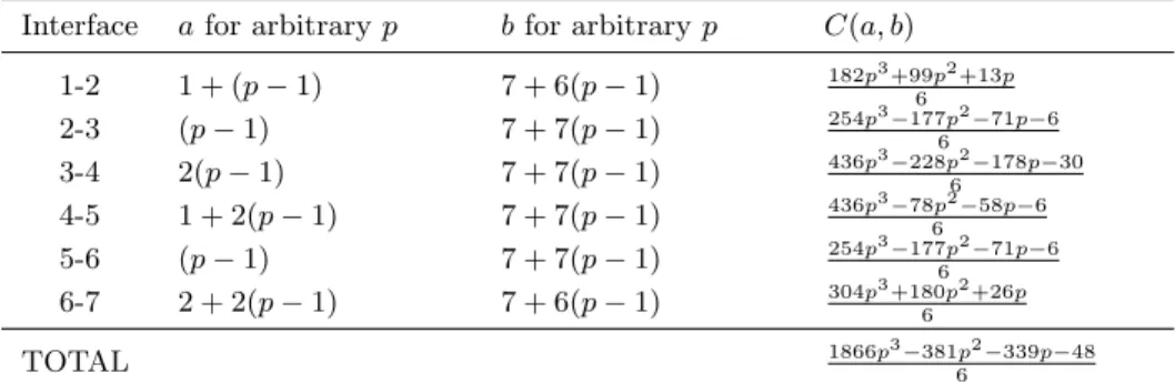
have to follow the order, but the direction (left to right or right to left) is not relevant to the result, so we may assume that we are proceeding from right to left. For a summary of the results, see Table 4. Having all the terms, it is now possible to assemble the final formula:
Table 4: Computational cost incurred by interface elimination for arbitraryk Interface afor arbitraryp bfor arbitraryp C(a, b)
1-2 1 + (p−1) 7 + 6(p−1) 182p3+996p2+13p 2-3 (p−1) 7 + 7(p−1) 254p3−1776p2−71p−6 3-4 2(p−1) 7 + 7(p−1) 436p3−228p62−178p−30 4-5 1 + 2(p−1) 7 + 7(p−1) 436p3−786p2−58p−6 5-6 (p−1) 7 + 7(p−1) 254p3−1776p2−71p−6 6-7 2 + 2(p−1) 7 + 6(p−1) 304p3+1806p2+26p TOTAL 1866p3−3816p2−339p−48
T(p, k) =T(k,0) +k12p 6+ 72p5+ 198p4+ 1558p3−441p2−277p−24 6 (8) Thus: T(p, k) =16p 6+ 96p5+ 264p4+ 864p3+ 533p2+ 93p 6 +k12p6+ 72p5+ 198p4+ 1558p3−441p2−277p−24 6 (9)
which completes the proof.
Lemma 4.2. The computational complexity of the hypergraph grammar driven solver for prob-lems with point singularities is equal to O(N), whereN is the number of unknowns.
Proof. The proof relies on Lemma 4.1 and transformsT(p, k) into a function ofN. In order to achieve this goal, we first need to determine the relationship between the number of elements Neand the number of redinement levelsk. The initial mesh fork= 0 has eight elements. Each new refinement level adds a layer of six new elements. Thus:
Ne(k) = 8 + 6k (10)
Since each element contains 4 degrees of freedom associated with its vertex, 4(p−1) degrees of freedom associated with its edges and (p−1)2 degrees of freedom associated with its interior, we multiply number of elements and number of degrees of freedom per element.
N(Ne, p) = (8 + 6k)((p−1)2+ 4(p−1) + 4) =O(p2+kp2) (11) Substituting this result inT(p, k) we receive:
T(p, N) =O(Np4) (12)
Since p can be treated as a constant and in fact, due to numerical side-effects is very rarely greater than nine, we receive:
T(N) =O(N) (13)
which proves the linear complexity.
5
Estimation of the memory usage
Memory usage can be estimated following the same pattern as in the previous section. Order of the memory usage of the solver can be well-approximated by computing the count of non-zero entries in the matrix. Since we do not store zero values, the real space usage is the function of non-zero entries (NZ). NZ at a given stage can be expressed as a function of previously definedaandb, like in Equation 14.
NZ(a, b) =a(a+ 1)
2 +a(b−a) (14)
Applying the same reasoning as in terms of computational complexity leads as to the following equation: MEM(k, p) =NZ(k, p) =1 2(12p 4+ 48p3+ 11p2+ 35p+ 4) +k1 2(105p 2−29p−8) (15) =O(p4+kp2) =O(N)
6
Generalization to the three dimensional grids
As an estimation of the exact computational cost for the three dimensional solver would be a very strenuous task, we restrict ourselves to a rough approximation of the computational complexity.
Lemma 6.1. Computational complexity of the sequential solver with respect to the number of degrees of freedomN and polynomial order of approximationpfor a three dimensional grid with point singularity is equal toT(p, N) =O(Np6).
Proof. A three dimensional element has number of degrees of freedom over an element edge of the order of O(p), the number of degrees of freedom over an element face of the order of O(p2) and the number of degrees of freedom over an element interior of the order ofO(p3). The computational complexity of elimination of the interior-related degrees of freedom is of the order ofO((p+p2+p3)2p3) =O(p9). The computational complexity of the static condensation is of the order ofO(Nep9), whereNedenotes the number of elements. The remaining faces and edges are eliminated level by level (layer by layer), and the computational complexity of elimination of a single level is of the order ofO((p2+p)3) =O(p6). The number of elementsNe is of the order of O(Ne) =O(pN3), and the number of levelsk is of the order ofO(k) =O(Np3) thus the
total computational complexity is of the order ofO(Nep9+kp6) =O(Np6+Np3) =O(Np6) which completes the proof.
7
Conclusions and future work
This paper contains a proof of the linear computational cost of the proposed direct solver algorithm executed on theh-refined computational grids with point singularities. This results show that theh-refined grids can be solved in linear costO(Np3) as opposed to the traditional solver algorithms delivering O(Np4+N1.5) cost for regular grids. The theoretical estimates has been proven by a series of experiments for p = 2, p = 3 and 1−8 point singularities. An interesting attempt would be to estimate solver’s complexity in case of different type of singularities such as edge singularities. AcknowledgementsThe work presented in this paper has been supported by Dean’s grant no. 15.11.230.106.
References
[1] P. R. Amestoy, I. S. Duff, J. Koster, and J.Y. L’Excellent. A fully asynchronous multifrontal solver using distributed dynamic scheduling. SIAM Journal of Matrix Analysis and Applications, 23(1):15–41, 2001.
[2] P.R Amestoy, I.S. Duff, and J.Y L’Excellent. Multifrontal parallel distributed symmetric and unsymmetric solvers. Computer Methods in Applied Mechanics and Engineering, 200(184):501– 520, 2000.
[3] K Bana´s. Scalability Analysis for a Multigrid Linear Equations Solver, volume 4967. Springer Berlin Heidelberg, 2008.
[4] L. Demkowicz. Computing With Hp-adaptive Finite Elements. Vol. 1: One and Two Dimensional Elliptic and Maxwell Problems. Chapman & Hall CRC, Texas, 2006.
[5] L. Demkowicz, J. Kurtz, D. Pardo, M. Paszy´nski, W. Rachowicz, and A. Zdunek. Computing With Hp-adaptive Finite Elements. Vol. 2: Frontiers: Three Dimensional Elliptic and Maxwell Problems with Applications. Chapman & Hall CRC, Texas, 2006.
[6] I. S. Duff and J. K. Reid. The multifrontal solution of indefinite sparse symmetric linear systems.
ACM Transactions on Mathematical Software, (9):302–325, 1983.
[7] I. S. Duff and J. K. Reid. The multifrontal solution of unsymmetric sets of linear systems. Inter-national Journal of Numerical Methods in Engineering, (5):633–641, 1984.
[8] A. Habel and H. J. Kreowski. May We Introduce to You: Hyperedge Replacement.Lecture Notes in Computer Science, 291:5–26, 1987.
[9] B Irons. A frontal solution program for finite-element analysis.International Journal of Numerical Methods in Engineering, 1970(2):5–32, 1970.
[10] D. Pardo. Integration of hp-adaptavity with a two grid solver: applications to electromagnetics. PhD thesis, The University of Texas at Austin, 2004.
[11] A. Paszynska, E. Grabska, and M. Paszynski. A Graph Grammar Model of the hp Adaptive Three Dimensional Finite Element Method. Part I. Fundamenta Informaticae, 114(2):149–182, 2012. [12] A. Paszynska, E. Grabska, and M. Paszynski. A Graph Grammar Model of the hp Adaptive Three
Dimensional Finite Element Method. Part II.Fundamenta Informaticae, 18(2):183–201, 2012. [13] A. Paszynska, M. Paszynski, and E. Grabska. Graph Transformations for Modeling hp-Adaptive
Finite Element Method with Mixed Triangular and Rectangular Elements.Lecture Notes in Com-puter Science, 5545:875–884.
[14] M. Paszynski, D. Pardo, and V.M. Calo. A direct solver with reutilization of LU factorizations for h-adaptive finite element grids with point singularities. Computers and Mathematics with Applications, 65(8):1140–1151, 2013.
[15] M. Paszynski, D. Pardo, and A. Paszynska. Parallel multi-frontal solver for p adaptive finite ele-ment modeling of multi-physics computational problems.Concurrency And Computation-Practice And Experience, 1(1):48–54, 2010.
[16] M. Paszynski and R. Schaefer. Graph grammar-driven parallel partial differential equation solver.
Concurrency And Computation-Practice And Experience, 22(9):1063–1097, 2010.
[17] G. Slusarczyk and A. Paszynska. Hypergraph Grammars in hp-adaptive Finite Element Method.
Procedia Computer Science, 18(4):1545–1554, 2013.
[18] B. Strug, A. Paszynska, and M. Paszynski. Using a graph grammar system in the finite element method. International Journal Of Applied Mathematics And Computer Science, 23(4):839–853, 2013.
[19] A. Szymczak, A. Paszynska, and P. Gurgul. Graph Grammar Based Direct Solver for hp-adaptive Finite Element Method with Point Singularities. Procedia Computer Science, pages 1594–1603, 2013.