Petrônio Cândido de Lima e Silva
Scalable Models for Probabilistic
Forecasting with Fuzzy Time Series
Belo Horizonte - Minas Gerais
July, 2019
Petrônio Cândido de Lima e Silva
Scalable Models for Probabilistic Forecasting with
Fuzzy Time Series
Final thesis presented to the Graduate Pro-gram in Electrical Engineering of the Federal University of Minas Gerais in partial fulfill-ment of the requirefulfill-ments for the degree of Doctor in Electrical Engineering.
Federal University of Minas Gerais - UFMG Graduate Program in Electrical Engineering - PPGEE Machine Intelligence and Data Science Laboratory - MINDS
Supervisor: Frederico Gadelha Guimarães
Co-supervisor: Hossein Javedani Sadaei
Belo Horizonte - Minas Gerais
July, 2019
have no merit alone neither did nothing in our life by ourselves. Because this I dedicate this work to the wide web of people that somehow helped me to become what I am. When I remember the people around me in my life, with varying degrees of closeness, I realize that it is almost impossible to separate what is my own and what is influence absorbed from
others. Because of this, I am continuously meditating about all my ancestors (also my parents in law) and my friends. It’s always on my mind their disposition to help and their
sacrifices to offer better life conditions to their sons, actions that paved the road I’m walking now. I’m grateful to all of you!
Acknowledgements
I would like to thank all my familly, but at first place my parents Joaquim Cândido and Édina Lúcia that are the main responsible for this achievement. You have no idea the respect, admiration and love I have for you. You are my heros! My brothers André and Ivana, my best friends since ever and forever and people that always inspired me. My parents in law, Antônio Dourado and Arlete Fraga, precious gifts that life gave me and I love and keep inside my heart.
My grandfathers Olavo Cândido and Otávio Perpétuo and my grandmothers Maria da Conceição (Lia) and Maria Salomé (Nina), in memoriam.
My precious jewel of light, my wife Nikaelle Fraga, I’m really devoted to you! You suffer with me each step of this odyssey, each pain and each victory. You deserve more credits for this than me, for having supported me and encouraged me to follow my dreams. You give meaning to my favorite quote:Ubi thesaurus tuus est, ibi cor tuum est. I love you! All my uncles, especially those from BH who were close to me during this journey: João Domingos, Maria Vita, Geralda Magela and Alencar Sanches (no, I didn’t forget about those from VGP and SSA, I love you!). All my cousins, especially Bruno Araújo and Alexandra Ank, thank you for everything! My sister-in-law Ingrid and my godchildren João Rafael and Antônio Nicolau, thanks for the good vibes.
My advisor Prof. Dr. Frederico Gadelha Guimarães, the best advisor ever and really a gifted person. I’m really proud to be your student and it’s a honor to have the opportunity to learn with you! Best wishes also for his wife Rúbia Pereira and his lovely daughter Laura.
My co-advisor Prof. Dr. Hossein Javedani Sadaei, a fantastic person which to a person who helped me and taught me a lot, also possibly the world’s greatest specialist on Fuzzy Time Series. It’s a privilege to count on you!
My lifelong best friends Prof. Dr. Gefter Thiago, Prof. Dr. Márcio Ramos (Bisa) and Prof. Rodrigo Carneiro Brandão. Even living so far and been so unplugged, my thoughts will always be with you! You are the best guys ever!
All professors and staff of the PPGEE - UFMG and my teammates on MINDS - Machine Intelligence and Data Science Laboratory, very special and careful people!
Cristiano Leite, Ivan Reinaldo, Rúbia Reis, Leonardo Augusto, Giulia Zanon, Maria Victória, Fernando Galindres, Roozbeh, Kossar, Omid Orang, Babak and Bruno Alberto. Thank you very much!
All colleagues and students of IFNMG - Instituto Federal do Norte de Minas Gerais. I will not nominate to avoid any omission, except for these special guys: Paulo Vitor (PV), Felipe (Bolinha) and Patrícia Lucas, also my colleagues at PPGEE.
Finally, my kittens Perrengo, Yôda, Salém and Vingador, my companies during the long nights writing this work. Meow!
“Simplicity is a great virtue but it requires hard work to achieve it and education to appreciate it. And to make matters worse: complexity sells better” (Edsger Wybe Dijkstra)
Abstract
No campo da previsão de séries temporais os métodos mais difundidos baseiam-se em predição por ponto. Esse tipo de previsão, no entanto, tem um sério inconveniente: ele não quantifica as incertezas inerentes aos processos naturais e sociais nem outras incertezas decorrentes da captura e processamento dos dados. Por isso nos últimos anos os métodos de previsão intervalar e probabilística têm ganhado a atenção dos pesquisadores, particularmente nas ciências climáticas e na econometria. Mas outro inconveniente vem do fato de grande parte dos métodos de previsão probabilística serem métodos de caixa preta e demandarem simulações estocásticas ou ensembles de métodos preditivos que são computacionalmente despendiosos.
Por outro lado, o volume (número de registros) e a dimensionalidade (número de variáveis) dos dados vêm alcançando magnitudes cada vez maiores, graças ao barateamento dos dispositivos computacionais de captura e armazenamento de dados, um fenômeno conhecido como Big Data. Tais fatores impactam diretamente no custo de treinamento e atualização dos modelos e, para séries temporais com essas características, a escalabilidade tornou-se um fator decisivo na escolha dos métodos preditivos.
Nesse contexto emergem os métodos de Séries Temporais Nebulosas, que vêm em crescente expansão nos últimos anos dado os seus resultados acurados, a facilidade de implementação dos métodos, o seu baixo custo computacional e a interpretabilidade de seus modelos. Os métodos de Séries Temporais Nebulosas têm sido utilizados em áreas como previsão de demanda energética, indicadores e ativos de mercado, turismo entre outras. Mas há lacunas na literatura de tais métodos referentes a escalabilidade para grandes volumes de dados e previsão probabilística e por intervalos.
A presente tese propõe novos métodos escaláveis de Séries Temporais Nebulosas e investiga a aplicação desses modelos na previsão por ponto, intervalar e probabilística, para uma ou mais variáveis e para mais de um passo à frente. Os parâmetros e hiperparâmetros dos métodos são discutidos e são apresentadas alternativas de ajuste fino dos modelos. Os métodos propostos são então comparados com as principais técnicas de Séries Temporais Nebulosas e outros modelos estatísticos utilizando dados ambientais e do mercado de ações. Os modelos propostos apresentaram resultados promissores tanto nas previsões por ponto quanto nas previsões por intervalo e probabilísticas e com baixo custo computacional, tornando-os úteis para um vasta gama de aplicações.
Palavras-chave: Séries Temporais Nebulosas, Previsão Probabilística, Escalabilidade, Pre-visão por Intervalo.
Abstract
In the field of time series forecasting, the most known methods are based on point forecasting. However, this kind of forecasting has a serious drawback: it does not quantify the uncertainties inherent to natural and social processes neither other uncertainties caused by the data gathering and processing. Because this in last years the interval and probabilistic forecasting methods have been gaining more attention of researches, specially on environmental and economical sciences. But these techniques also have their own issues due to the methods being black-boxes and requiring stochastic simulations and ensembles of multiple forecasting methods which are computationally expensive.
On the other hand, the data volume (number of instances) and dimensionality (number of variables) have reached magnitudes even greater, due to the commoditizing of the capturing and storing computational devices, in a phenomenon known as Big Data. Such factors impact directly on the model’s training and updating costs, and for time series with Big Data characteristics, the scalability became a decisive factor in the choosing of predictive methods.
In this context the Fuzzy Time Series (FTS) methods emerge, which have been growing in recent years due to their accurate results, easiness of implementation, low computational cost and model explainability. The Fuzzy Time Series methods have been applied to forecast electric load, market assets, economical indicators, tourism demand etc. But there is a lack on FTS literature regarding interval and probabilistic forecasting.
This thesis proposes new scalable Fuzzy Time Series methods and discusses its application to point, interval and probabilistic forecasting of mono and multivariate time series, for one to many steps ahead. The parameters and hyper-parameters are discussed and fine tunning alternatives are presented. Finally the proposed methods are compared with the main Fuzzy Time Series techniques and other literature approaches using environmental and stock market data. The proposed methods obtained promising results on point, interval and probabilistic forecasting and presented low computational cost, making it useful for a wide range of applications.
Keywords: Fuzzy Time Series, Probabilistic Forecasting, Interval Forecasting, Scalable Models.
Preface
“From my part I know nothing with any certainty, but the sight of the stars makes me dream.”
— Vincent Van Gogh
When Prof. Fred suggested me to study Fuzzy Time Series - I need to confess - I became excited. Because one of the most fascinating issues on scientific research is to deal with uncertainty. Uncertainty is pervasive, omnipresent and self propagated. Pliny the Elder, early on first century of Cristian Age, stated that “the only certainty is the uncertainty”. The mankind expanded the boundaries of the knowledge and some uncertainties could be reduced or eliminated. Others, however, remain irreducible. And here we are!
I always felt uncomfortable with the mechanistic and deterministic view of the world. The advances of science have forced us to assume some limitations of our knowledge and accept the separation between our known-knowns, the known-unknowns and even of the unknown-unknowns. We know now that we live in a fuzzy and probabilistic world.
And until here we just talked about the present and the past. Things get even more interesting when we try to look ahead and predict the future. If we can’t measure accurately some natural, social and economical processes, due to instrumentation limitations for example, and these processes are also intrinsically non-deterministic, these uncertainties combined make the forecasting task complex and barely precise.
The fog of uncertainty becomes yet more dense as the forecasting horizon goes away: the forecasting methods need to into take account all uncertainties on present to forecast ranges of possibilities on future. When we look more than one step in the future the forecasting method should consider all possible combinations in the range of variation of each past step - and this increases the complexity and the output uncertainty.
With this research problem in hand, many ideas in mind, and a lot of excitement, we expect to give some contributions to this field. We focused on non-deterministic processes and assume that all measurements are not completely accurate, every single value actually represents a fuzzy neighborhood. We propose to bring the fuzzy time series to the domain of probabilistic forecasting.
List of abbreviations and acronyms
ARIMA Autoregressive Integrated Moving Average BSTS Bayesian Structural Time Series
CRPS Continuous Ranked Probability Score
DEHO Distributed Evolutionary Hyperparameter Optimization
FIG Fuzzy Information Granule
FIG-FTS Fuzzy Information Granule Fuzzy Time Series FLR Fuzzy Logical Relationship
FLRG Fuzzy Logical Relationship Group
FTP Fuzzy Temporal Pattern
FTPG Fuzzy Temporal Pattern Group
FTS Fuzzy Time Series
HOFTS High Order Fuzzy Time Series IFTS Interval Fuzzy Time Series
LHS Left Hand Side
MAE Mean Absolute Error
MAPE Mean Average Percent Error MVFTS Multivariate Fuzzy Time Series
PWFTP Probabilistic Weighted Fuzzy Temporal Pattern
PWFTPG Probabilistic Weighted Fuzzy Temporal Pattern Group PWFTS Probabilistic Weighted Fuzzy Time Series
RMSE Root Mean Squared Error
UoD Universe of Discourse
WHOFTS Weighted High Order Fuzzy Time Series WIFTS Weighted Interval Fuzzy Time Series WMVFTS Weighted Multivariate Fuzzy Time Series
List of symbols
Y ∈Rn the crisp time series data
n=|V| the number of variables ofY, univariate ifn = 1or multivariate ifn > 1
y(t)∈Y an individual instance of Y on timet
F ∈A˜ Linguistic time series produced by Y fuzzyfication
f(t)∈F an individual instance ofF on timet, such thatf(t) ={Aj |µAj(y(t))≥
α∀Aj ∈A˜}
U = [l, u] the Universe of Discourse of a univariateY, where the lower bound is
l= minY and the upper bound is u= maxY.
T ∈N+ the total length of Y
t∈T the time index
k∈N+ the number of partitions of U
α∈[0,1] the Alfa-Cut, the minimal membership grade to be considered in fuzzy-fication process
Ω∈N+ the Model order, the number of time series lags used by model
L the lag indexes
µAj :U →[0,1] the fuzzy membership function for fuzzy set Aj,j = 1..k
˜
A the linguistic variable for univariateY Aj ∈A˜ the individual fuzzy sets in A˜, j = 1..k
V the set of variables of a multivariateY
Vi ∈ V an individual variable ofY,i= 1..n
∗V ∈ V the target variable (or endogenous variable) ofY
αi Alpha-Cut for each Vi ∈ V, i= 1..n
e
Vi the linguistic variable for each Vi ∈ V, the group of fuzzy sets,i= 1..n
AVi
j ∈Vei the individuals fuzzy sets in Vei, i= 1..n and j = 1..ki
M the FTS model, including the linguistic variable A˜and the knowledge model
|M| the model parsimony, the amount of parameters of the model
H ∈N+ The forecasting horizon, i.e, the number of steps to predict ahead
ˆ
y(t+ 1)∈Rn a point forecast for time t+ 1
I= [l, u] a prediction interval for time t+ 1 with lower bound l ∈R and upper
bound u∈R
Contents
1 Introduction . . . 21
1.1 Objectives . . . 24
1.2 Work structure . . . 24
1.3 Main contributions . . . 25
2 Fuzzy Time Series . . . 27
2.1 Fuzzy Time Series common processes . . . 28
2.2 Universe of Discourse Partitioning . . . 31
2.2.1 Universe of Discourse U . . . 31
2.2.2 Membership function µ . . . 32
2.2.3 The number of partitions k . . . 33
2.2.4 The partitioning method - Π . . . 34
2.3 The Fuzzyfication Process . . . 36
2.4 Knowledge Extraction, Representation and Inference . . . 37
2.4.1 The Order Ω, Lags L and Seasonality . . . 37
2.4.2 Matrix Models . . . 38
2.4.3 Rule Models . . . 39
2.4.4 Weighted Rule Models . . . 40
2.4.5 Neural Networks Models . . . 41
2.4.6 Metaheuristics. . . 42
2.4.7 Hybrid Approaches . . . 42
2.5 The Deffuzyfication Process . . . 42
2.6 Data Transformations for Pre and Post Processing . . . 44
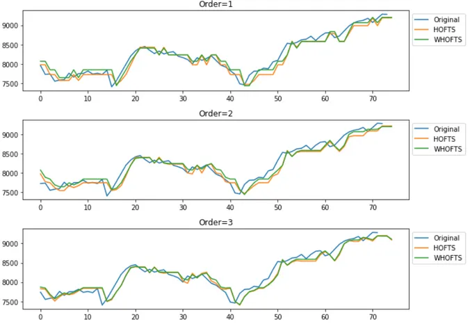
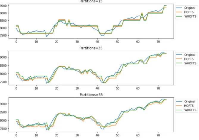
2.7 A Conventional High Order Fuzzy Time Series Method - HOFTS . . . 45
2.7.1 Training Procedure . . . 45
2.7.2 Forecasting Procedure . . . 46
2.7.3 The Weighted Extension - WHOFTS . . . 47
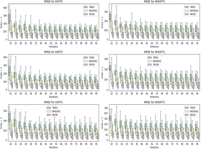
2.8 Computational Experiments . . . 48
2.8.1 Evaluation Measures for Point Forecasts . . . 48
2.8.2 Hyperparameter Grid Search . . . 49
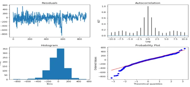
2.8.3 Residual Analysis . . . 50
2.9 Conclusion . . . 51
3 Probabilistic Forecasting . . . 59
3.1 The Point Forecast Limitations . . . 60
3.2 Interval Forecasts . . . 61
3.2.1 Accuracy Measures for Interval Forecasts . . . 62
3.3.2 Weighted [I]F T S . . . 67
3.4 Probability Distribution Forecasts . . . 69
3.4.1 Accuracy Measures for Probabilistic Forecasts . . . 74
3.4.2 Fuzzy Time Series Methods With Probabilistic Background. . . 75
3.5 The Ensemble FTS Method . . . 76
3.5.1 Training Procedure . . . 77
3.5.2 Forecasting Procedure . . . 78
3.6 Computational Experiments . . . 79
3.6.1 Hyperparameter Grid Search . . . 81
3.6.2 Interval Forecasting Benchmarks . . . 82
3.6.3 Probabilistic Forecasting Benchmarks . . . 84
3.7 Conclusion . . . 86
3.7.1 Methods limitations . . . 87
4 Probabilistic Weighted Fuzzy Time Series . . . 91
4.1 Fuzzy Empirical Probabilities . . . 92
4.2 PWFTS Training procedure . . . 94
4.3 Forecasting Procedure . . . 96
4.3.1 Probabilistic Forecasting Procedure . . . 97
4.3.2 Interval forecasting procedure . . . 98
4.3.3 Point forecasting procedure . . . 100
4.4 PWFTS extensions . . . 101
4.4.1 Many steps ahead forecasting . . . 101
4.4.2 High order models . . . 102
4.5 Computational Experiments . . . 104
4.5.1 Hyperparameter Grid Search . . . 104
4.5.2 Point Forecasting Benchmarks . . . 105
4.5.2.1 Residual Analysis . . . 106
4.5.3 Interval Forecasting Benchmarks . . . 107
4.5.4 Probabilistic Forecasting Benchmarks . . . 108
4.6 Conclusion . . . 109
4.6.1 Method limitations . . . 110
5 Scalability And Hyperparameter Optimization . . . 113
5.1 Computational Clusters . . . 114
5.2 Scalable Models With Distributed Execution . . . 115
5.2.1 Distributed Testing With Sequential Models . . . 116
5.2.2 Distributed Models . . . 117
5.2.2.1 Distributed training Procedure . . . 118
5.3 Distributed Evolutionary Hyperparameter Optimization. . . 120
5.4 Computational Experiments . . . 124
5.4.1 Speed Up Of Distributed Methods . . . 124
5.4.2 Convergence of DEHO approach . . . 125
5.5 Conclusion . . . 127
5.5.1 Method limitations . . . 128
6 Multivariate Models . . . 129
6.1 Multivariate FTS Methods . . . 130
6.1.1 Fuzzy Information Granules . . . 130
6.2 The Conventional Multivariate Fuzzy Time Series method . . . 131
6.2.1 Training Procedure . . . 132
6.2.2 Forecasting Procedure . . . 133
6.2.3 Interval forecasting for MVFTS . . . 134
6.2.4 Weighted Multivariate FTS - WMVFTS . . . 135
6.3 Fuzzy Information Granule Fuzzy Time Series F IG-FTS . . . 136
6.3.1 Training Procedure . . . 137
6.3.2 Forecasting Procedure . . . 139
6.3.3 Method discussion . . . 140
6.4 Computational Experiments . . . 141
6.4.1 SONDA models settings . . . 141
6.4.2 Malaysia models settings . . . 142
6.4.3 Results . . . 144
6.5 Conclusion . . . 144
6.5.1 Method limitations . . . 147
7 Conclusion . . . 151
7.1 Summary of contributions . . . 153
7.2 Summary of methods limitations . . . 154
7.3 Future Investigations . . . 154
7.4 Publications . . . 155
7.4.1 Journal Papers . . . 155
7.4.2 Conference Papers . . . 155
7.4.3 Software Libraries . . . 156
7.4.4 Short Courses and Talks . . . 156
References . . . 159
Appendix A Monovariate Benchmark Datasets . . . 179
B.1 SONDA dataset . . . 181 B.2 Malaysia dataset . . . 182
21
Chapter 1
Introduction
“In the strict formulation of the law of causality - if we know the present, we can calculate the future - it is not the conclusion that is wrong, but the premise.”
— Werner Heisenberg
A significant part of scientific applications demand the forecasting of natural, social and economical processes and there is an extensive literature on forecasting meth-ods and models. Such methmeth-ods are also preceded by many processes as instrumentation, measurement, storing, aggregation, etc. However, a great recurrent problem is how to deal with the uncertainty generated or captured in each step of this task, and measure how it spreads. Makridakis and Taleb[2009] stated that “Statistical models underestimate uncertainty, sometimes catastrophically”, by assuming, for example, that events are inde-pendent, forecasting errors are tractable, the variance of forecasting errors is finite, known and constant.
In these natural and social processes the uncertainty can be intrinsic or extrinsic and is classified, by Georgescu [2014], in two categories: the epistemic uncertainty and the ontological uncertainty. The ontological uncertainty represents the intrinsic and irreducible uncertainty of a process defined basically as the non-deterministic behavior – randomness and stochasticity – that usually is modeled by the probability theory.
Contrarily, the epistemic uncertainty represents the extrinsic and reducible sources of uncertainty on a process like vagueness, lack of information and imprecision due to measurement errors, sensor calibration, rounding and limitations of numerical precision, among others. Another possibility is the conversion of continuous processes to discrete processes. This conversion is not lossless and some uncertainty is imputed on converted data. The epistemic uncertainty can be modeled by the fuzzy theory.
This is the case of data preprocessing tasks, for example. Very often time series datasets need to be aggregated by some time resolution (daily, hourly, etc) and this
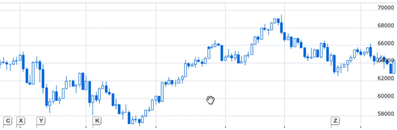
Figure 1 – Candlestick chart for IBOVESPA. Source: Google Finance1
aggregation also introduces the epistemic uncertainty on data. A good example are the financial time series that summarize all transactions of a whole day in four numbers: opening, minimum, maximum and closing prices. This method is an attempt to represent the volatility (e. g. the uncertainty) of the price value inside a certain time window and is also a tool for detecting patterns on data, the Candlestick Graph techniques, as shown in Figure 1. Sometimes the aggregation is even more aggressive and all the values are summarized into one, the average or median value, hiding all information about the volatility. When this data is used as input for fitting a forecasting model the extrinsic uncertainty is introduced.
The forecasting methods propagate the input uncertainties on their outputs and compromise the reliability of the forecast. Despite these points, the majority of forecasting methods are concerned with one step ahead point forecasting without output uncertainty measures. When the many steps ahead forecasting is considered, the uncertainty grows yet more and affects the accuracy and reliability of models. This effect becomes even worst as the forecasting horizon becomes wider.
This fact led to the development of methods for Probabilistic ForecastingGneiting and Katzfuss [2014] and Interval Forecasting Chatfield [1993], to deal with forecasting uncertainty by estimating distributions of possible values instead of a unique point forecast. However, traditional methods of probabilistic forecasting require the use of parametric models with distribution assumptions, as in Bayesian Inference, or costly estimation techniques and Monte-Carlo simulations. Probabilistic forecasting has been used in areas such as weather forecasting (Fraley et al. [2011] and Leutbecher and Palmer[2008]) eletric load forecasting (Hong and Fan [2016], Hong et al. [2016] and Liu et al. [2015]), wind power generation prediction (Pinson et al.[2006] and Netto et al. [2016]) and hydrological forecasting (Laio and Tamea[2007]).
Side by side with the uncertainty representation in time series forecasts, some
1
https://www.google.com/financeq=INDEXBVMF%3AIBOV&ei=zHz2WOmMKODrep_bgbAI. Access in 18/04/2017
23
other factors became prevailing in the evaluation of predictive methods, such as Big Data scalability and model explainability. The Big Data phenomenon emerged in the late 2000s decade Lynch [2008] calling attention to new demands on data analysis brought by the growth of data volume, dimensionality and variety. This revolution was possible due to the advances on the technologies of data capturing and storage, as well as its commoditizing, allowing the distributed management of amounts of data never seen before.
But traditional forecasting methods, and even some newer ones, were not designed to deal with such high volume of data. The most critical issues were the high dimensionality (dozens of hundreds of attributes) and volume (hundreds of millions or billions of samples) Qiu et al. [2016]. Such data volume cannot be grounded on a single machine memory and demands a distributed architecture of storage and processing. New technologies emerged to tackle these issues, for instance the Map Reduce based frameworks Dean and Ghemawat [2008], a divide-and-conquer approach which is the basis of Hadoop clustersWhite [2012], where the processing units also act as storage units of the data subsets using commodity and cheap hardware assets.
The Big Data issues do not stop on data volume and, indeed, the velocity and variability of the data must be seriously considered when developing forecasting mod-els. Many sources of data have non-stationary behaviors, meaning that their statistical properties may change along the time. Some models are time-variant, they are specially designed to be self-adaptable and evolve as the data change. But the majority of the conventional methods are time-invariant and need to be retrained periodically depending on the variability of the data, what can be problematic given the computational cost of the training and adapting procedures. Yet more critical is the data with Concept Drifts [Gama et al., 2014], which have high volume with high velocity and need to be adaptable to new behaviors in feasible time.
Another traditionally neglected aspect of the forecasting methods also started to gain more attention in recent years: the explainability. With the expansion of the machine learning methods enabled to tackle Big Data, another issues came up to the light: black-box methods started to find legal barriers or adoption resistance due to its lack of transparency and auditability [Leslie,2019, EC AI HLEG,2019]. Diversely, the white-box methods can help in the knowledge extraction and simplification of complex temporal patterns, besides being easily auditable.
The exposed scenario favored the rising of the Fuzzy Time Series (FTS) methods Song and Chissom[1993b], which have been drawing more attention and relevance in recent years due to many studies reporting its good accuracy compared with other models Singh and Prabakaran [2008]. Fuzzy Time Series are soft-computing methods that produce data-driven, non-parametric, simple, computationally cheap and readable models for time series analysis and forecasting. FTS methods are also an approach to deal with the epistemic
uncertainty, as on the time-aggregation case of the financial time series. The fuzzyfication of data gives a more flexible representation to the individual measures, embracing the range of possible value fluctuations not covered by the single values.
Despite the great improvements published in the FTS literature in the recent years, there are still some notable lacks. Interval and probabilistic forecasting, specially for many steps ahead, are not properly explored, besides the absence of scalable methods to tackle big multivariate time series. There is, indeed, a plethora of soft-computing forecasting methods. But very few of them are flexible enough to incorporate scalable point, interval, probabilistic and multivariate forecasting, with one to many steps ahead, for univariate and multivariate time series. This research opportunity is exploited in this work by the proposition of new FTS methods and their subsequent applications on several case studies, including financial, environmental and energy time series.
1.1
Objectives
The main goal of this thesis is to develop a scalable probabilistic forecasting approach based on the Fuzzy Time Series methods, providing a flexible computational framework for applications with uncertainties. Specific goals are divided in:
• Identify the strengths and weaknesses of the main FTS approaches presented in literature;
• Identify extension opportunities on known probabilistic forecasting methods;
• Introduce the Probabilistic Weighted Fuzzy Time Series, a new method family that exploits uncertainties on datasets to capture time series patterns and translate them into the rule-based knowledge system (the Probabilistic Weighted Fuzzy Logical Relationship Groups);
• Improve PWFTS scalability in order to enable it to deal with big time series by proposing a distributed processing design with the Map/Reduce paradigm;
• Extend the PWFTS method to enable multivariate time series using Fuzzy Informa-tion Granules.
1.2
Work structure
This thesis is organized as follows:
• Chapter 2 - Fuzzy Time Series presents a contextual background on Fuzzy Time Series methods and discusses the most relevant methods in literature;
1.3. Main contributions 25
• Chapter 3 - Probabilistic Forecasting introduces the probabilistic forecasting concepts and main techniques, reviewing the surrounding literature. In Section 3.3 the Interval Fuzzy Time Series method is proposed for binding the fuzzy uncertainty on forecasts, and in Section3.5the EnsembleFTS method is proposed to probabilistic forecasting;
• Chapter 4 - Probabilistic Weighted Fuzzy Time Series introduces the Prob-abilistic Fuzzy Time Series method for generating the ProbProb-abilistic Weighted Fuzzy Temporal Pattern rules and a method to generate one step ahead probabilistic fore-casts; in Section 4.3.2 the previous method is extended to create prediction intervals and in Section 4.3.3 a simple heuristic to produce point forecasts is presented . Section 4.4 presents extensions for many steps ahead forecasting and high-order models. The characteristics and parameters of the methods are discussed in Section 4.5;
• Chapter 5 - Scalability And Hyperparameter Optimization proposes a dis-tributed approach for PWFTS, based on Map/Reduce paradigm and computational clusters, enabling it to deal with big time series. In Section5.3the Distributed Evolu-tionary Hyperparameter Optimization (DEHO) is proposed, employing evoluEvolu-tionary algorithms with the distributed processing to improve the performance.
• Chapter 6 - Multivariate Models proposes an extension for multivariate time series using Fuzzy Information Granules (FIG) and an incremental universe of discourse partitioner. With this extension PWFTS can be used for multivariate forecasting in a Multiple Input/Multiple Output (MIMO) design or monovariate forecasting in a Multiple Input/Single Output(MISO) design.
• Chapter 7 - Conclusion the findings are summarized and overall conclusions are given, as well as the contributions, known limitations and future investigations.
1.3
Main contributions
This research presents contributions to the Forecasting and Fuzzy Time Series research fields, whose the most important are summarized below:
• development of the Probabilistic Weighted Fuzzy Time Series - PWFTS, which is a new non-parametric, data driven and highly accurate forecasting method, the first FTS method in the literature that integrates point, interval and probabilistic forecasting in the same model, for one to many steps ahead;
• a new representation method for fuzzy temporal rules, with weights on the precedent and the consequent of the rules, reflecting its a priori and a posteriori empirical probabilities and aiding with model explainability;
• new defuzzyfication methods capable to produce probability distributions, prediction intervals and point forecasts and multivariate output using Fuzzy Information Granules (FIG);
• the pyFTS library Silva et al. [2018]2 for Python programming language, an open
and free framework to facilitate the development of new models and help on research reproducibility;
• application of the proposed methods in the forecasting of renewable energy and environmental processes;
27
Chapter 2
Fuzzy Time Series
“There’s nothing worst than a sharp image of a fuzzy concept” — Ansel Adams
This chapter aims to introduce the Fuzzy Time Series methods and review the relevant literature, offering a soft background on the key concepts and models on this research field.
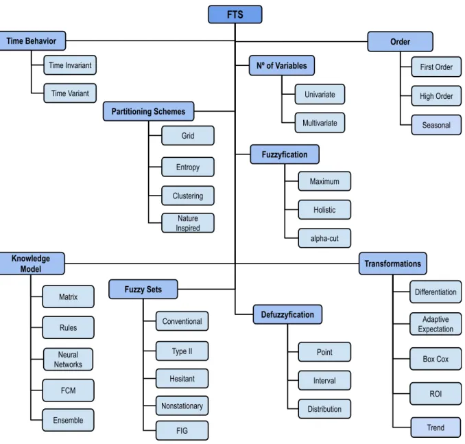
The name Fuzzy Time Series (FTS) can be used to refer to F, a time series composed by fuzzy linguistic terms, or the family of non-parametric forecasting methods introduced by Song and Chissom [1993b] based on Fuzzy Set theory Zadeh[1965]. These methods are easy to implement and very flexible, affording ways to deal with numeric and non-numeric data. FTS methods have been commonly employed in forecasting of university enrollments (Song and Chissom [1993b], Song and Chissorn [1994], Ismail and Efendi [2011]), stock markets (Sadaei et al. [2016b], Lee et al. [2013a], Chen [2014], Sun et al. [2015], Talarposhti et al. [2016], Efendi et al. [2013]), tourism (Lee and Javedani [2011]), electric load (Ismail et al. [2015], Sadaei et al. [2017]), seasonal time series [Song [1999], Chang [1997]] among many others. There are still some gaps in FTS methods (Sadaei [2013] and Georgescu [2010]) related with methodological problems but many of them have been approached in more recent studies Sadaei et al. [2016a]. There are several categories of FTS methods whose main features and its variations can be seen in Figure 2, and will be discussed in the remaining sections.
The most important categories of FTS methods are related with their the time behavior. The time invariant models are the ones used when the Universe of Discourse and data behavior does not change with time, as in stationary time series. Non stationary time series, in its turn, require time variant models as proposed in Song and Chissorn [1994] and Wong et al. [2010]. This research is focused on time invariant models and hereinafter all models discussed belongs to it. However, Time Variant models are not discarded for future investigations.
FTS Order Nº of Variables Time Behavior First Order High Order Univariate Multivariate Time Invariant Time Variant Seasonal Trend Partitioning Schemes Clustering Entropy Grid Nature Inspired Transformations Differentiation Adaptive Expectation Box Cox ROI Knowledge Model Rules Matrix FCM Neural Networks Fuzzy Sets Type II Conventional Hesitant Nonstationary Ensemble Defuzzyfication Point Interval Distribution FIG Fuzzyfication Maximum Holistic alpha-cut
Figure 2 – A brief taxonomy of FTS methods
This chapter also focus only on monovariate and non Big Data time series. The multivariate and Big Data methods will be discussed in the following chapters. In the next section the main processes of the FTS are introduced and discussed.
2.1
Fuzzy Time Series common processes
The definition of Fuzzy Time Series, from Song and Chissom [1993b], starts with a univariate time seriesY ∈R1, for t = 0,1, ..., T, where the Universe of Discourse U is delimited by the known bounds ofY, such that U = [min(Y),max(Y)]. UponU, k fuzzy setsAj, forj = 1..k, are defined and each one with its own membership function µAj. F is called a Fuzzy Time Series overY if f(t) =µAj(y(t)) is the collection of fuzzyfied values of Y for j = 1..k andt = 0,1, ..., T. The group of fuzzy sets Aj, for j = 1..k, can also be
2.1. Fuzzy Time Series common processes 29
the linguistic variable.
FUZZY SETS - Ã CRISP DATA - Y PARTITIONING FUZZYFICATION FUZZYFIED DATA - F KNOWLEDGE MODEL - 𝓜 KNOWLEDGE EXTRACTION NUMBER OF PARTITIONS - k PARTITIONING METHOD - Π MEMBERSHIP FUNCTION - μ ORDER - Ω LEGEND ■ PROCEDURES ■ DATA ■ PARAMETERS ■ HYPERPARAMETERS PRE PROCESSING LAG INDEXES - L α-CUT
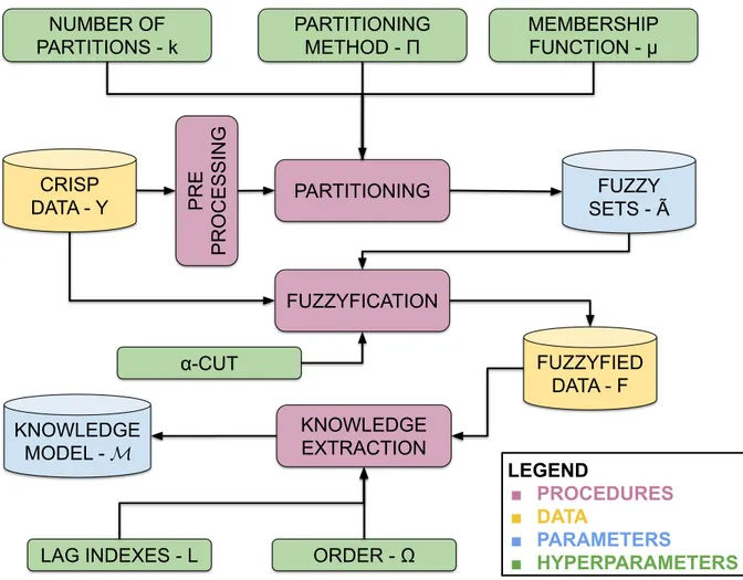
Figure 3 – Generic time invariant Fuzzy Time Series training procedure and its components
Song and Chissom [1993a] proposed the first FTS methodology and the following authors basically extended or modified some steps of the method. A generic method can be extracted from the wide range of variations of FTS methods by splitting the FTS approach in two main procedures, the training and forecasting methods. The training method, illustrated in Figure 3, has the basic objective to create the linguistic variableA˜
and a knowledge representation of the time series dynamics. These two objects compose the FTS model M. The main components of this process are listed below:
Step 1 - Pre-processing: First, one or more pre-processing data transformations can be applied to input data Y, responsible to reduce noise, detrending, or de-seasonalize, or change the U, etc. Several methods contain these operators and their impact will be discussed in detail in Section 2.6.
Step 2 - Partitioning: The most important process of the training is executed, the parti-tioning. This process is responsible to split the universe of discourse U into k fuzzy sets Aj, creating the linguistic variable A˜used to describe Y. There are many ways
that the partitioning can be performed, and the most important are discussed in Section 2.2.
Step 3 -Fuzzyfication: With the linguistic variableA˜the crisp dataY can be transformed in a linguistic representation, the fuzzy time series F where each f(t) ∈ F is a fuzzyfied version of y(t) ∈Y. Details of the fuzzyfication are discussed in Section 2.3.
Step 4 - Knowledge Extraction and Representation: The second most important pro-cess is the knowledge extraction. This propro-cess is responsible to induce the knowledge model M by performing a pattern recognition over F and learning the temporal patterns between Ω lags, whose indexes are identified byL, and their consequent ones. The most important learning algorithms and knowledge models are discussed in Section 2.4.
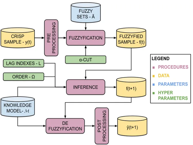
Once the linguistic variable A˜ is defined and the FTS modelMwas learned, new samplesy(t)∈U can be presented to produce a forecast yˆ(t+ 1). The generic forecasting procedure is illustrated in Figure4, and its main components are listed below:
Step 1 - Pre-processing: First, one or more pre-processing and post-processing data transformations can be applied to input sample y(t)(the data transformations are discussed in Section 2.6).
Step 2 -Fuzzyfication: The fuzzyfication procedure follows the same schema of the training procedure and it is discussed in Section 2.3.
Step 3 - Inference: The inference engine deeply depends on the knowledge model M. Indeed, the learning algorithm, the knowledge model and the inference engine are intrinsically correlated, and they are discussed in Section2.4. The aim of the inference process is to producef(t+ 1), candidate fuzzy sets (and other additional information, as weights) to represent the future crisp value y(t+ 1).
Step 4 - Deffuzyfication: The deffuzyfication process aims to transform thef(t+ 1) to a crisp numeric estimate yˆ(t+ 1) for the real (but unknown) value y(t+ 1). The deffuzyfication usually also depends on the inference engine but there are common methods discussed in Section 2.5. The present work extended the possibilities of deffuzyfication to beyond of point forecasting, proposing methods for prediction intervals I and probabilistic distributions P.
Step 5 - Post-processing: Finally, one or more post-processing data transformations can be applied to output forecast yˆ(t+ 1) (the data transformations are discussed in Section 2.6).
2.2. Universe of Discourse Partitioning 31
FUZZY SETS - Ã
CRISP
SAMPLE - y(t) FUZZYFICATION
INFERENCE FUZZYFIED SAMPLE - f(t) KNOWLEDGE MODEL- 𝓜 DE FUZZYFICATION LEGEND ■ PROCEDURES ■ DATA ■ PARAMETERS ■ HYPER PARAMETERS f(t+1) ŷ(t+1) POST PROCESSING PRE PROCESSING ORDER - Ω
LAG INDEXES - L α-CUT
Figure 4 – Generic time invariant Fuzzy Time Series forecasting procedure and its compo-nents
The main hyperparameters which affect these processes are listed in Table 1. The selection of the values for these hyperparameters affects the training process and the parameters of the model, including its accuracy and parsimony (the length of the model). In the following sections each one of these processes are discussed in detail recurring to the most relevant works in the FTS literature, while its strengths and drawbacks are highlighted.
2.2
Universe of Discourse Partitioning
This process aims to split the Universe of Discourse U and to create the linguistic variableA˜, composed by the fuzzy sets Aj,j = 1..k. This is the most important process of
the FTS approach and the following sections detail its main sub-processes and parameters.
2.2.1
Universe of Discourse
U
The natural definition of the Universe of Discourse is U = [min(Y),max(Y)], but it is common that the upper and lower bounds be exceeded by a confidence margin.
Alias Parameter Process
k ∈N+ Number of partitions (fuzzy sets) Universe of Discourse Parti-tioning
µ:U →[0,1]
Membership function, measures the membership of a valuey ∈U to a fuzzy set
Universe of Discourse Parti-tioning, Fuzzyfication
Π Partitioning method Universe of Discourse
Parti-tioning
α∈[0,1]
the α-cut, the minimal membership grade to take account on fuzzyfication process
Fuzzyfication
Ω∈N+ Order, the number of lags Knowledge model
L∈Ω×N− Time lag indexes Knowledge model
Table 1 – Common hyperparameters for FTS methods
Then, it can be established as U = [l, u], with the lower bound as l = min(Y) +ld, where
ld= min(Y)·0.2(exceeding the original lower bound by 20%) and the upper bound as
u= max(Y) +ud, where ud= max(Y)·0.2 (exceeding the original upper bound by 20%).
Even considering just time invariant methods in this work and a stationary time series Y, it is natural that the testing U will be a little different from the training U, sometimes by a small fraction of the original values. Even on stationary processes the presence of outliers cannot be discarded. The objective of these exceeding margins ld
and ud is to help in the fuzzyfication process of the forecasting procedure, in order to
accommodate fluctuations in the bounds of the known U.
2.2.2
Membership function
µ
Once U has been defined, three hyperparameters will determine the creation ofA˜: the number of partitionsk, the membership function µand the partitioning scheme. The membership function µ:U →[0,1] defines how much a crisp value belongs to a fuzzy set, in terms of the membership grade[0,1]. Some options of fuzzy membership functions are shown in Table 2, and simple partitioning using these functions are shown in Figure 5. The real impact of the membership function on accuracy is low, it will be demonstrated empirically later on this work, but the chosen of the correctµcan help in the readability and explainability of the model.
Many other kinds of fuzzy sets were presented in the literature and new FTS methods were developed using them, as instance Type 2 fuzzy sets [Huarng and Yu, 2005, Bajestani and Zare, 2011], Hesitant fuzzy sets [Bisht and Kumar, 2016], non-stationary fuzzy sets [Alves et al., 2018], etc. These fuzzy sets and the methods developed with them, however, are considered out of the scope of this research.
2.2. Universe of Discourse Partitioning 33
Name Parameters Definition
Singleton c, the central value µ(x, c) =
1 if x=c
0 if x6=c
Triangular a: lower bound,b:
mid-point, c: upper bound µ(x, a, b, c) = 0 if x≤a x−a b−a if a ≤x≤b c−x c−b if b ≤x≤c 0 if c≥x Trapezoidal
a: lower bound,b: top-left, c: top-right,d up-per bound µ(x, a, b, c, d) = 0 if x≤a x−a b−a if a≤x≤b 1 if b≤x≤c d−x d−c if c≤x≤d 0 if d≥x
Gaussian m: midpoint,d: spread µ(x, m, d) = exp−(x2−md2)2
Table 2 – Most common fuzzy membership functions
Figure 5 – UoD Partitioning using different membership functions
2.2.3
The number of partitions
k
The selection of the hyperparameter k impact directly on the model accuracy and parsimony, as discussed in Duru and Yoshida [2012]. The number of partitions impact on the model parsimony directly and, for instance, given a rule model the maximum number of rules is the cartesian product between the fuzzy sets Aj ∈A˜for each order Ω.
There is a non-linear relationship between k and the model accuracy, a trade off between specific accuracy (bias) and overall generalization (variance). A small value of k
will generate too few fuzzy sets to representY correctly, making the model Munderfit by producing a gross generalization with simplistic patterns. A high value of k will generate too much fuzzy sets, exceeding the needed to represent Y and makeing the model M
number ofk must be optimized for each problem, balancing the accuracy and the model parsimony, since this last value affects the computational performance as the number of parameters grows.
The impact of the U partitioning can also be seen by other perspectives: the model human readability and model explainability. In his seminal work, Miller [1956] stated that the human being, on average, can learn7±2 concepts. In other words, the linguistic variable A˜ to be reasonable for human understanding must have around this number of fuzzy sets. But this, depending on the range ofU and the behavior ofY, may be a very small number of partitions. Otherwise, the explainability does not depend on how much humans can learn from M but how easily the forecastings produced can be explained, as a white box model. In this last case the type of the knowledge representation of Mhas greater impact than the number of fuzzy sets in A˜.
A study of the linguistic characterization of time series can be found in Novák [2016a]. using Fuzzy Transform (Perfilieva [2006]) to generate linguistic summaries of time series. A study on mining information from fuzzyfied linguistic time series can be found inNovák[2016b], where are presented the impacts of fuzzyfication on the knowledge extraction.
2.2.4
The partitioning method -
Π
The partitioning method will determine, for each fuzzy set, their length, midpoints and bounds and also have impact on accuracy. The simplest partitioning scheme – the division of the data range ink equal length intervals – is called Grid Partitioning and was proposed in Song and Chissom [1993b]. In the Grid Partitioning, U is divided in k+ 2
even intervalsu1, u2, ..., uk whose midpoints are c1, c2, ..., ck. Then with these k intervals
k overlapped fuzzy sets A1, A2, ..., Ak are defined using triangular membership functions
whose parameters are cj−1, cj, cj+1 for each j = 2..k−1.
Some works use simple heuristics to define k or even the lengths of the fuzzy sets. Huarng[2001] use a grid partitioning approach, but it proposes an empirical method to find the ideal number of partition lengths according to the magnitude ofU, in a work that was the first to deeply discuss the impact of the partitioning on FTS forecast accuracy. Several other works used this or define other simple heuristic forU partitioning, see for instance Chang[1997], Huarng and Yu [2005],Rubio et al. [2016],Cheng and Chen [2018].
U partitionings where the fuzzy sets have unequal lengths are also present in the literature.Cheng et al.[2006] employ a fixed value ofkbut the entropy of data that defines the best midpoints for the fuzzy sets, which also use trapezoidal membership functions. This method is known by Entropy Partitioning and is also employed inCheng et al.[2008b] andChen et al.[2014]. The statistical approaches yet count withIsmail et al. [2015], which
2.2. Universe of Discourse Partitioning 35
Figure 6 – Partitioning using different approaches within the same sample
determine the length of the fuzzy sets proposing a method based on data quantiles, and Yang et al. [2017a] which use a Chi-Square distribution do identify the fuzzy sets number and lengths.
Clustering techniques are used in several works, as Fuzzy C-Means in Li et al. [2008], Askari and Montazerin [2015], Bas et al. [2015], Sun et al. [2015],Yolcu and Lam [2017], Fuzzy K-Medoids in Dincer and Akkuş [2018], Self Organizing Maps in Bahrepour et al. [2011], and other methods as in Saberi et al. [2017] and Bose and Mali[2017].
The use of metaheuristics, especially of nature-inspired optimization approaches, is also spread in the literature. Particle Swarm Optimization is used by Davari et al.[2009], Kuo et al. [2009], Hsu et al. [2010], Huang et al. [2011], Zhang et al. [2018b], Genetic Algorithms inChen and Chung [2006], Enayatifar et al. [2013],Zhang et al. [2018a], and other less known methods such as Harmony Search in Talarposhti et al. [2016], Jiang et al. [2017] and Imperialist Competitive in Sadaei et al.[2017].
A sample of different partitioning schemes on the same data can be seen in Figure 6. The partitioning method has influence on the model accuracy, parsimony and readability but its computational cost must be also considered. The Grid Partitioning gives a uniform distribution of the fuzzy sets over U but, if in one hand it is computationally cheaper, however it may not represent the importance of some data regions accordingly. It is probable that some specific regions of U have more variance than others, depending onY
behavior, and some regions may be better represented having more fuzzy sets than others. It also can not be denied that some approaches are computationally expensive, as the clustering and metaheuristics ones, and in Big Data scenarios this may be prohibitive. Despite the fact that the Grid Partitioning should be always the first approach to start with, due to its simplicity and small cost, the fine tuning of FTS models can not exclude
more sophisticated methods.
Once the linguistic variable A˜ is created, the fuzzyfication process can be started. This process and its parameters are discussed in the next section.
2.3
The Fuzzyfication Process
This process aims to transform the crisp numerical time series Y into a linguistic time seriesF, also known as fuzzy time series. There are few, but important, variations of the fuzzyfication method.
The initial FTS methods, for instance Song and Chissom [1993b], Chen [1996] andYu[2005], only considered one fuzzy set in fuzzyfication process, for instancey(t)∈Y, the one with the greatest membership grade. More specifically:
f(t) = Aj |µAj(y(t)) = max{µA1(y(t)), . . . , µAk(y(t))} (2.1) This method helps to control overfit, reducing the number of spurious patterns generated by low membership grades fuzzy sets. However, it can also contribute to underfit the learning by eliminating fuzzy sets which are very close to the maximum grade. It is possible to deduce that some relevant information can be lost when several minor membership grades are discarded.
A contrasting method is the holistic fuzzyfication, where all the membership grades, despite their magnitude, are considered. The fuzzyfied valuef(t)is the the vector of the y(t) membership grades with respect to each Aj ∈A˜:
f(t) = [µA1(y(t)), . . . , µAk(y(t))] (2.2) The holistic fuzzyfication can help to the learning overfit, because even very small membership grades, which can be considered insignificant for that fuzzy set, are considered. An intermediate approach can be achieved by using the α-cut hyper-parameter. The
α-cut represents the minimal value of the membership grade that will be accepted in fuzzyfication, while membership values below the α-cut will not be considered.
f(t) = Aj |µAj(y(t))≥α ∀Aj ∈A˜ (2.3) The α-cut makes the sensibility of the fuzzyfication process adjustable and the user can control it, unlike the maximum membership and the holistic methods. The fuzzyfication method is significant in the search of the training best fit, controlling the accuracy and models parsimony. Particularly, the method of Carvalho Jr and Costa Jr
2.4. Knowledge Extraction, Representation and Inference 37
[2017] makes an explicit use of theα-cut parameter and conduct a comprehensive study of its impact on the method accuracy.
Once the crisp data Y is converted to the fuzzy time series F the process of knowledge extraction and representation is ready to start. This process and its variations are discussed in the next section.
2.4
Knowledge Extraction, Representation and
Inference
This section aims to investigate the several approaches in the literature that were used to learn and represent temporal patterns found on the fuzzyfied data F. Looking back to Figures 3and 4, the fuzzy sets and the fuzzyfication process may be interpreted as a feature extraction layer that precedes a pattern recognition and inference layer, that is finally succeeded by a reconstruction layer – the deffuzyfication process. Besides small variations, the fuzzyfication and deffuzyfication do not differ among the methods. But the way these methods learn and store the patterns suffer a strong variation among them.
By far, most of FTS methods make use of simple heuristics to learn the temporal patterns from the fuzzyfied data and store the learned patterns using rules or matrices. But it can not be denied that there are many other backends for the knowledge extraction and representation in FTS models: metaheuristics, neural networks, fuzzy cognitive models, hybrid approaches with traditional statistical models, etc. In the following sections the most relevant methods with their variations will be discussed.
2.4.1
The Order
Ω
, Lags
L
and Seasonality
First it is needed to consider the hyperparameters order Ω and the lag indexes
L. These parameters also impact directly on the model accuracy and parsimony. The number of lags Ω indicate how much past information is available to the model M to recognize the possible temporal patterns and make a forecast. Very short-term memory or even memory-less processes will require just the last time lag, consequently produce a first order model (Ω = 1). Processes with longer memories will require more lags and produce higher-order models (Ω>1).
Otherwise, the hyperparameter Lindicates which past lags are taken into account during the forecast. Not always the most recent time lags contain the best information to predict the near future and this is particularly important for seasonal time series, where
L will indicate the time lags which have periodically similar values. Initially the values of L can be extracted from the Autocorrelation Function (ACF), examining the most significant lags. However, this number can be optimized with fewer lags.
TheHigh Order Fuzzy Time Series - HOFTS defines the High Order Fuzzy Logical Relationships - HOFLR as LHS → RHS form, where LHS is the set of f(t−L(Ω−
1)), ..., F(t−L(0)) fuzzy sets, and the RHS is f(t+ 1), the group of consequent fuzzy sets. We can find these kind of models in Chen [2002], Chen and Chung [2006],Jilani and Burney[2008],Li et al. [2008], Egrioglu et al.[2010],Bahrepour et al. [2011],Enayatifar et al.[2013], Chen et al. [2014],Chen and Chen [2015b],Ye et al. [2016], Lee et al.[2017], Bose and Mali[2017], Sadaei et al.[2017], Guney et al. [2018], Cheng and Chen [2018], Yang et al. [2018],Zhang et al. [2018b].
Seasonal models try to represent cyclical behaviors, e. g, repeated values of the time series in regular periods. Seasonal Fuzzy Time Series - SFTS methods, make use of the L parameter to represent the seasonal periods as lag indexes. SFTS were first proposed in Song et al. [1997], basically by defining a seasonal index in L, such that
f(t+ 1) =f(t−L). Chang[1997] proposed a method for capturing fuzzy trend and fuzzy seasonal indexes using Fuzzy Regression. Other seasonal methods include Tseng et al. [1999],Song [1999], Lee and Javedani[2011].
The hyperparameters Ω and L are used across several learning algorithms and knowledge representation models, which are the ways the patterns of F are extracted, stored and inferred. As stated before, the knowledge representation ofMis important due to the human readability and explainability. White-box models have high explainability and human readability but suffer to represent high dimensional data and very complex dynamics of temporal patterns. In other hand the black-box models have low explainability and almost zero human readability (which are unfortunately subjective concepts) but are very efficient in representing high-dimensional spaces and complex temporal dynamics.
2.4.2
Matrix Models
The original work of Song and Chissom [1993b] used a Fuzzy Relationship Matrix to represent the temporal dynamics of the fuzzy time series F. In this method, each sequential pair f(t−1), f(t)∈F is grouped in Fuzzy Logical Relationships - FLR1. The
FLR are fuzzy rules that describe a temporal pattern f(t−1)→f(t), or Ai →Aj where
the Left Hand Side - LHS of the rule (or the precedent) Ai is the fuzzyfied historical
value at timet−1and the Right Hand Side - RHS of the rule (or the consequent)Aj the
fuzzyfied value at timet. The Ai →Aj rule can be read as “IF f(t−1) isAi THEN f(t)
isAj”. The F dataset will generate T −1 FLRs, as the fuzzyfication process of Song uses
the maximum membership method.
1 It should be noted that the nomenclature of FLR may be misunderstood. The wordrelationship, in
the fuzzy sets research field, has a different meaning than that used bySong and Chissom. Fuzzy relationships are operations between fuzzy sets, e. g. projection and cylindrical extension, well discussed inKlir and Yuan [1995]. The intention of the authors was to nominate a temporal pattern between two fuzzy sets, a temporal succession relationship, not a logical fuzzy relationship. However this nomenclature is spread in the FTS literature and will be kept on this text.
2.4. Knowledge Extraction, Representation and Inference 39
Then, for each FLR Ai →Aj a matrix Rt =ATi ×Aj =aij will be created, with
dimensions k×k where aij = min{µAi(t), µAj(t−1)} for i, j = 1, ..., k and t = 1, ..., T. This matrix contains the fuzzy membership of the FLR for all fuzzy sets. The Operation Matrix R(t, t−1) is computed as the union of all relationship matrices Rt, such that
R(t, t−1) =ST
t=1Rt. The Operation Matrix contains the memberships of all FLR for all fuzzy sets.
The inference using Fuzzy Relational Matrices demands to find the membership of the relation f(t−1) → f(t) on R(t, t−1), such that f(t) = f(t −1)◦R(t, t−1), where ◦is the Max-Min fuzzy relational operator. The operation f(t−1)◦R(t, t−1) = maxj{mini{µAi(f(t−1)), rij}} for i, j = 1, ..., k and rij ∈ R(t, t−1) produces a vector with the memberships of f(t) for all Aj fuzzy sets.
Several other studies use this heuristic to extract Fuzzy Relational Matrices, for instance Song et al. [1997],Jeng-Ren Hwang et al. [1998], Song [1999], Chen and Hwang [2000], Chen and Chung [2006], Cheng et al. [2008b], Jilani and Burney [2008], Davari et al. [2009], Qiu et al. [2011], Cheng and Li[2012], Qiu et al. [2013] and Chuang et al. [2014].
2.4.3
Rule Models
A great improvement was given by Chen[1996] who proposes a simplification of Song and Chissom’s method by creating the Fuzzy Logical Rule Groups (FLRG), making the forecasting process cheaper by avoiding the use of matrix manipulations. The FLRG represent the knowledge base (rule base) of the model and are human readable and easy to interpret.
Create the Fuzzy Logical Relationship Group - FLRG with the formLHS →RHS, where all FLR’s with the same LHS are grouped and the RHS is the set of possible fuzzy sets that can follow the LHS set. The LHS → RHS pattern can be read as “IF
F(t −1) = LHS THEN ∃Aj ∀Aj ∈ RHS | F(t) = Aj” . An example of rule set is
demonstrated on (2.4), given k= 6. A0 →A1 A1 →A1, A2 A2 →A4 A3 →A2, A3, A5 A4 →A3, A4 A5 →A4 (2.4)
The inference using [Chen,1996], produces a forecast for the one step ahead value
theLHS =Ai. The RHS of the FLRG will average all the possible fuzzy sets that follow
Ai when f(t) = Ai, i. e., the forecast f(t+ 1) is the RHS set of the selected FLRG.
The Chen’s FLRG models allowed a compact and human readable representation of the time series behavior using fuzzy rules, which could in principle be used by business experts and researchers in knowledge extraction, for instanceLee et al. [2006]. But there is also another good reason to prefer the Chen’s model over the Song and Chissom, the performance. The relation matrix dimension grows as the number of UoD partitions grows and the curse of dimensionality tends to impact negatively on the computational time spent on forecasting large datasets.
Several other works use this heuristic to extract rule models, for instance Chen [2002],Huarng and Yu[2004],Lee et al. [2006],Li et al.[2008],Hsu et al.[2010],Bahrepour et al.[2011], Huang et al.[2011],Sun et al. [2015],Sadaei et al. [2016b], Lee et al.[2017], Yang et al.[2017a],Bose and Mali[2017],Carvalho Jr and Costa Jr[2017]. Other heuristics are also present in the literature, such as the use of the APriori algorithm inCheng and Chen[2018].
2.4.4
Weighted Rule Models
The generation of FLRG from the fuzzyfied data in FTS model has, at least, two drawbacks: the losing of rule’s recurrence and their chronological order. Thus at the forecasting process a very recurrent pattern of data has the same importance of a unique occurrence pattern. Moreover, newer and older patterns also have the same weight in the forecast.
To fix these drawbacks Yu [2005] proposed the Weighted Fuzzy Time Series
(WFTS) model by including weights on FLRG’s. These weights are monotonically increasing and have a smoothing effect, giving more importance to the most recent data in forecasting process. TheWeighted Fuzzy Logical Relationship Group - WFLRG has the same structure as the FLRG but weights wj are associated with each fuzzy setAj ∈RHS.
The works of Ismail and Efendi [2011] and Efendi et al. [2013] have presented the
Improved Weighted Fuzzy Time Series (IWFTS) model and changed the way in which the weights are assigned to the RHS rules on Yu’s model. The main difference is that the weights are calculated by the recurrence of each rule, discarding the chronological order. The Exponentially Weighted Fuzzy Time Series (EWFTS) method, proposed by Sadaei et al. [2014] and Talarposhti et al. [2016], replaces the linear weight growth of WFTS model by an exponential growth.
Lee et al. [2013b] proposed a broad generalization of the weighted methods with thePolynomial Fuzzy Time Series- PFTS. This method demands the coefficient fitting by optimization techniques but is capable of approximating WFTS, IWFTS and EWFTS
2.4. Knowledge Extraction, Representation and Inference 41
methods.
Cheng et al. [2008b] and Cheng et al. [2009] proposed the Trend Weighted Fuzzy Time Series - TWFTS which separates the FLRG’s in three trends - no change, up trend and down trend - and assigns a weight to them according to the recurrence of the trend on the FLRG. Another contribution of these works is the Adaptive Expecta-tion step, after defuzzyficaExpecta-tion the forecast value a transformaExpecta-tion is employed such as
Adaptative_F orecast(t) =F(t−1) +h·[F(t)−F(t−1)], where F(t) is the forecasted value, F(t−1)is the true past value and his weight parameter that smooth the transition between the actual value and the forecasted value. Table 3 presents a summary of the weighting methods in FTS. Method Weights WFTS Pn1 i=1i , 2 Pn i=1i , ... , n Pn i=1i IWFTS f1 Pn i=1fi , f2 Pn i=1fi , ... , fn Pn i=1fi EWFTS Pnc0 i=1ci , c1 Pn i=1ci , ... , cn−1 Pn i=1ci TWFTS f1 Pn i=1fi , f2 Pn i=1fi , ... , fn Pn i=1fi Table 3 – Weighting schemes for Fuzzy Time Series
2.4.5
Neural Networks Models
Neural Networks are black-box methods known to be the state-of-the-art in several pattern recognition domains. Its ability to deal with high dimensional and complex domains makes it attractive for many FTS models, specially the ones that deal with many variables and time simultaneously, as the case of Egrioglu et al. [2009].
Simpler univariate methods can be found on Yolcu and Lam [2017] which used a single multiplicative neuron whose inputs are the fuzzyfied values of several time lags. Bas et al. [2015] and Bas et al. [2018] used a Pi-Sigma Network, a variation of the well known ANFIS network, trained with Particle Swarm Algorithm.
Another hybrid FTS architecture is proposed by Bas et al. [2015], the Fuzzy Time Series Network - FTS-N which proposes a new topology for high-order FTS with a network layout, somehow similar to an ANFIS network. The partitioning of UoD and the fuzzyfication of the data use FCM clustering and the overall network is trained with PSO, combined yet with an autoregressive layer.
More recently, the new Deep Learning models begin to interact with the FTS field. Starting with Tran et al. [2018], which proposed a method that uses Long-Short Term Memory networks as knowledge model, trained with Backpropagation Through The Time algorithm.Sadaei et al. [2019] proposed the Image FTS, where the fuzzyfied data of
several past lags are stacked to compose a binary image, which in turn is processed by a Convolutional Neural Network model trained by the backpropagtion method.
Fuzzy Cognitive Maps (FCM), developed by Kosko [1986], is a different kind of neural architecture inspired in the Mind Map tools, which is simpler than the Multilayered Neural Networks but also very powerful to represent nonlinear and causal behaviors. FCM are used as backend for FTS on Homenda et al. [2014], Homenda and Jastrzebska[2017], Yang and Liu[2018].
2.4.6
Metaheuristics
It was already seen in Section 2.2that metaheuristics are widely used to determine the best partitioning scheme. However metaheuristics also can be used to extract or optimize the knowledge model representation from the fuzzyfied data.
The already cited Kuo et al. [2009] also use Particle Swarm Optimization (PSO) to build optimal rule sets on the Hybrid Particle Swarm FTS - HPSO-FTS. The PSO metaheuristic is also used in other works to train neural models, as inBas et al. [2015], Yolcu and Lam [2017],Bas et al. [2018]. Genetic Algorithms to learn a matrix of weighted rules are employed in Ye et al. [2016].
The optimization of Ω and L are the focus of Enayatifar et al. [2013], which proposes theRefined High-order Weighted FTS with Imperialist Competitive Algorithm -RHWFTS–ICA, using evolutionary computing to optimize the number of lags for the high order seasonal FTS and the weights for adaptive expectation. The Adaptive Sine-Cosine Human Learning Optimization (ASCHLO) was used in Yang et al. [2018] for rule and weight induction.
2.4.7
Hybrid Approaches
Autoregressive and polynomial models were adopted in Chang[1997],Tseng et al. [1999],Askari and Montazerin[2015],Talarposhti et al. [2016]. These methods used classic optimization approaches to fit regression coefficients mixed with fuzzy terms.
Sadaei et al. [2016a] propose the ARFI–FTS, a hybrid approach that combines statistical method ARFIMA with FTS for forecasting of long-memory time series. Also Bas et al. [2015] contains a hybrid approach, combining its network model with an autoregressive layer.
2.5
The Deffuzyfication Process
The result of the inference is a set of f(t+ 1)possibilities, or rules involving it, to be converted in a crisp numerical value yˆ(t+ 1)that estimates the unknown value of
2.5. The Deffuzyfication Process 43
y(t+ 1). The deffuzyfication method aims to deliver ayˆ(t+ 1)∈U that meets the expected value, or the expected mean of the several patterns contained in f(t+ 1) forecast.
InSong and Chissom[1993b], the defuzzyfication process converts the membership vector f(t+ 1) into a scalar value on the universe of discourse. Taken the maximum membership values of f(t), with the following method:
1. If there is only one maximum, yˆ(t+ 1) will be the midpoint of the maximum membership fuzzy set;
2. If there are more than one consecutive maxima, yˆ(t+ 1) will be the mean of the midpoints;
3. Otherwise, yˆ(t+ 1) will be the weighted mean of the fuzzy sets midpoints with the memberships, such thatyˆ(t+ 1) =P
j∈f(t)µj·cj, where µj is the membership degree
and cj is the midpoint of the fuzzy set Aj ∈A˜
In the method ofChen [1996], the deffuzyfication is adapted to the following steps, given the f(t+ 1) =RHS of the selected FLRG:
1. If the RHS contains only one fuzzy set, yˆ(t+ 1) will be the midpoint of the set; 2. If the RHS contains more than one fuzzy set, yˆ(t+ 1) will be the mean of the
midpoints of these sets.
The above methods are considered the Simple Mean methods. For weighted rule models as Sadaei et al. [2014], for each rulei, the expected mean point Ei of the rule is
the weighted mean of the midpoints mpAj of their RHS consequents by the weights wij.
Ei = k
X
Aj∈RHS
wij ·mpAj (2.5)
When more than one pattern (in the case of rules) was found in the inference step the expected values of each pattern must be mixed. The simplest way is performing a Simple Mean, where iis each active rule of the model M, Ei is the expected mean point
of each rule i and |M| is the number of active rules in model M.
ˆ
y(t+ 1) =|M|−1 X
i∈ M
Ei (2.6)
The drawback of this method is to give the same importance for all patterns. In the Weighted Sum each pattern is weighted by its activation, where i is each active rule
![Figure 13 – [I]F T S many steps ahead interval forecasting procedure](https://thumb-us.123doks.com/thumbv2/123dok_us/10076976.2907663/69.892.138.793.650.1011/figure-i-f-steps-ahead-interval-forecasting-procedure.webp)
