Method for Computing Protein Binding Affinity

Paper COMP 160 presented at the

228th National Meeting of the American Chemical Society, August 22–26, 2004, Philadelphia, PA

Method for Computing Protein

Binding Affinity

Charles F. F. Karney‡and Jason E. Ferrara

Sarnoff Corporation, Princeton, NJ 08543-5300

Stephan Brunner§

Locus Pharmaceuticals, Inc., Blue Bell, PA 19422-2700

Abstract

A Monte Carlo method is given to compute the binding affinity of a ligand to a protein. The method involves extending configuration space by a dis-crete variable indicating whether the ligand is bound to the protein and a special Monte Carlo move which allows transitions between the unbound and bound states. Provided that an accurate protein structure is given, that the protein-ligand binding site is known, and that an accurate chemical force field together with a continuum solvation model is used, this method provides a quantitative estimate of the free energy of binding.

∗_{This work was supported, in part, by the U.S. Army Medical Research and}

Introduction

Consider a drug molecule, the ligand L, binding reversibly to a pro-tein P, via

L + P LP.

In equilibrium, reaction is governed by the dissociation constant Kd =

[L][P] [LP] .

Define the binding affinity as pKd = −log₁₀

K_d/N_A

1 kmol m−3

,

where NA is the Avogadro constant.

Goal of this work: given • protein structure • ligand binding site • chemical force field • solvation model

compute Kd. Benefits are

• screen drug leads prior to synthesis • guide the design of drug leads

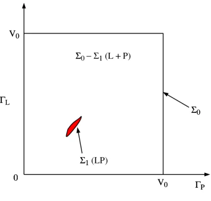
00 _VV 00 ΓΓ_LL ΓΓ_PP ΣΣ₀₀ ΣΣ11 (LP) ΣΣ₀ − Σ₁₁ (L ++ P) V V₀₀

Figure 1: Configuration space showing the volumes corresponding to the unbound molecules L + P and the complex LP.

Formulation

Consider a system of volume V0 consisting of a ligand molecule L and a protein molecule P in a solvent. The state of the system is given by Γ = [ΓL,ΓP], where ΓM represents the phase space

con-figuration of molecule M (position, orientation, conformation); see Fig. 1. In equilibrium, the system obeys the Boltzmann distribution1

Σ0 corresponds to all allowable configurations; Σ1 corresponds to

the LP complex. In the dilute limit V0 → ∞, we find2, 3, 4

Kd = 1 V0 R Σ0 exp[−βE0(Γ)]dΓ R Σ1 exp[−βE1(Γ)]dΓ , (1)

where E1(Γ) is the full energy of the system and E0(Γ) is the

“un-bound” energy, ignoring the interaction between L and P.

Combine the bound and unbound systems by extending phase space Γ → [Γ, λ]; λ = {0,1}.

Define canonical average by hXi = P λ R dΓ exp[−βEλ(Γ)]Xλ(Γ) P λ R dΓ exp[−βEλ(Γ)] .

Now Eq. (1) can be rewritten as Kd = 1 V0 hδλ0i hδλ1i , (2)

where δλµ is the Kronecker delta. Because the definition of Kd is

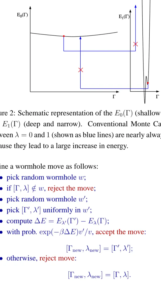
Wormhole Monte Carlo

We can compute the canonical averages in Eq. (2) using the Monte Carlo method5 to make steps from [Γ, λ] to [Γ0, λ0] with acceptance probability

min[1,exp(−β[Eλ0(Γ0) −Eλ(Γ)])].

However, the estimate of the Kd will be very poor, because

transi-tions between λ = 0 and 1 will be extremely rare; see Fig. 2.

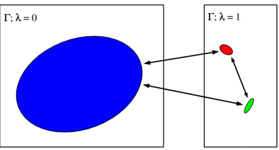
Remedy this problem by restricting the standard moves to changes in Γ only, and allowing changes in λ via “wormhole moves” which connect otherwise disconnected regions of configuration space. Wormhole moves combine two concepts

• squeezing Γ space is equivalent to decreasing E (via Jacobian

factor when transforming integrals),6, 7

• allowing direct jumps between wells (subject to “detailed

bal-ance”).8, 9

Define a set of wormhole regions w, w0, w00, . . . . These are subsets of [Γ, λ] space with configuration space volumes of v, v0, v00, . . . . Intersperse wormhole moves with regular Monte Carlo moves.

E E₀₀((ΓΓ)) _EE 11((ΓΓ)) ΓΓ ΓΓ

..

..

Figure 2: Schematic representation of the E0(Γ) (shallow and wide) and E1(Γ) (deep and narrow). Conventional Monte Carlo moves

betweenλ = 0 and1(shown as blue lines) are nearly always rejected because they lead to a large increase in energy.

Define a wormhole move as follows:

• pick random wormhole w;

• if [Γ, λ] ∈/ w, reject the move;

• pick random wormhole w0;

• pick [Γ0, λ0] uniformly in w0;

• compute ∆E = Eλ0(Γ0)− Eλ(Γ);

• with prob. exp(−β∆E)v0/v, accept the move: [Γnew, λnew] = [Γ0, λ0]; • otherwise, reject move:

ΓΓ; λλ = 1 ΓΓ; λλ = 0

Figure 3: Typical wormholes for the case illustrated in Fig. 2. The large ratio of the volume of the unbound wormhole compared to the bound wormholes compensates for the higher energy of the unbound configurations. This results in accepted wormhole moves between all the wormholes.

If the mean energy of configurations in w scales asβ−1 lnv+ const., the acceptance probability is O(1);

Finding the wormhole

In order for the wormhole method to be practical, we need a reliable way of choosing the wormholes. For simplicity take protein to be rigid and fixed. Fix the bond lengths and bond angles in the ligand and allow l bonds to rotate. Configuration of system is given by

• position of L (3), • orientation of L (3), • conformation of L (l).

• Total dimensionality is n = l + 6.

Carry out canonical Monte Carlo simulations with Eλ(Γ) separately

for λ = 0 and 1. For each λ, obtain a canonical set of configurations {Γ}. Fitn-dimensional ellipsoid to each{Γ}with center at the mean configuration hΓi. Compute the deviation from the mean, δΓ = Γ− hΓi, and compute a covariance matrix

hδΓδΓi = BBT.

Ellipsoids are a natural choice to use to fit the set of configurations: • The iso-density contours of the distribution in a harmonic well

are ellipsoids.

• It is easy to sample points randomly from an ellipsoid.

• Conversely, it is easy to test that a point lies inside an ellipsoid. • The volume of an n-dimensional ellipsoid is given by

vn = πn/2 (n/2)! n Y i=1 ai,

where ai is the length of ith semi-axis.

Test suitability of ellipsoid by demanding that O(1) of the config-urations sampled uniformly from it have energies close to its mean energy hEλ(Γ)i. If test fails, split {Γ} into two sets according to the

sign of δΓ projected along the largest semi-axis of the ellipsoid and construct new trial wormholes from each of these sets.

Method of finding wormholes depends on the samples “spanning” a volume of phase space. Requires that the dimensionality of phase space be sufficiently small. Thus

• Must use an implicit solvation model.

• Minimize number of degrees of freedom for conformational changes by fixing the bond lengths and bond angles.

How good are wormhole moves?

Example: p-amino-benzamidine (Fig. 4) bound to trypsin:

• Protein structure from trypsin-benzamidine complex, 1BTY10 (Fig. 5).

• At physiological pH, ligand is protonated (net charge of +1). • Amber 7 force field11, 12, 13 and GB/SA solvation model.14, 15, 16 • Find 16 unbound and 8 bound wormholes.

• Pick V0 = 0.39 × 10−18m3 .

• Binding affinity calculation of 5× 106 steps.

Data from binding affinity calculations. For every 1000 steps:

wormhole attempts 900

Γ ∈ w? 26

successful wormhole move 15

λ transition 0 → 1 → 0 3

Main cost is evaluation of E1(Γ). But the frequent Γ ∈/ w steps are

free! Thus

Cost of each λ transition ∼ 3× E1(Γ)

Wormholes are effective in making the transition between the bound and unbound systems.

Computational result: pKd = 7.99 ± 0.01

Experimental17, 18 result: pKd = 5.1± 0.1

+ NH NH N H 2 2 2

7.9 8 8.1 0 1 2 3 4 5 pK d (s) s × 106

Figure 6: Cumulative estimates pKd(s) obtained from the first s

steps of 5 independent Monte Carlo runs The dashed lines shows convergence as 1/√s to the mean value of 7.99.

Convergence

Repeat computation 5 times and plot the cumulative estimates of pKd based on the first s steps of each run; see Fig. 6. The converge

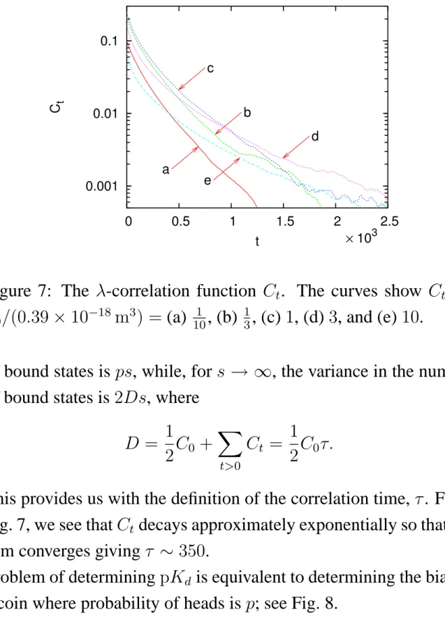
depends on how rapidly the switch between λ = 0 and 1 is made. This is determined by the λ-correlation function

Ct = h(λs − p)(λs+t − p)is,

where p = hδλ1i, λs is the value of λ at simulation step s and h. . .is

denotes an average over steps. Figure 7 shows Ct for several

0.001 0.01 0.1 0 0.5 1 1.5 2 2.5 C t t a b c d e × 103

Figure 7: The λ-correlation function Ct. The curves show Ct for

V0/(0.39 × 10−18 m3) = (a) ₁₀1 , (b) 1₃, (c) 1, (d) 3, and (e) 10.

of bound states is ps, while, for s → ∞, the variance in the number of bound states is 2Ds, where

D = 1 2C0 + X t>0 Ct = 1 2C0τ.

This provides us with the definition of the correlation time, τ. From Fig. 7, we see that Ct decays approximately exponentially so that the

0.7 0.8 0.9 1 0 2 4 6 8 10 12 14 h n /t n n × 103

Figure 8: Estimation of the bias of a coin with p = 0.443. Five independent runs are shown; hn (tn) is the number of heads (tails)

observed in n trials. The axes have been adjusted to allow the figure to be directly compared with Fig. 6.

Discussion

• Direct sampling of two physical systems, E1(Γ) and E0(Γ)

(compare with free energy perturbation theory).

• Accumulating 1 (in either hδλ0i or hδλ1i)

– no rare large values (high error) – no frequent small values (high cost)

• Can sample with E_λ∗(Γ) ≈ Eλ(Γ) and compensate in the

ca-nonical averages.

• Can apply standard Monte Carlo techniques

– preferential sampling – early rejection

– force bias – etc.

• Can extend to treat

– limited protein flexibility – ring flexibility in ligand

– protonation states (at constant pH) – tautomers

• Limitations

– explicit solvent not treated

References

[1] L. D. Landau and E. M. Lifshitz, Statistical Physics; Vol. 5 of Course of

Theoretical Physics; Pergamon Press, 2nd ed., 1969.

[2] M. Mezei and D. L. Beveridge, Ann. N.Y. Acad. Sci., 1986, 482, 1–23. [3] C. H. Bennett, J. Comp. Phys., 1976, 22, 245–268.

[4] H. Luo and K. Sharp, Proc. Nat. Acad. Sci., 2002, 99, 10399–10404.

[5] N. Metropolis, A. W. Rosenbluth, M. N. Rosenbluth, A. H. Teller, and E. Teller, J. Chem. Phys., 1953, 21, 1087–1092.

[6] M. A. Miller and W. P. Reinhardt, J. Chem. Phys., 2000, 113, 7035–7046. [7] Z. Zhu, M. E. Tuckerman, S. O. Samuelson, and G. J. Martyna, Phys. Rev.

Lett., 2002, 88, 100201.

[8] A. F. Voter, J. Chem. Phys., 1985, 82, 1890–1899.

[9] H. Senderowitz, F. Guarnieri, and W. C. Still, J. Am. Chem. Soc., 1995, 117, 8211–8219.

[10] B. A. Katz, J. Finer-Moore, R. Mortezaei, D. H. Rich, and R. M. Stroud,

Biochemistry, 1995, 34, 8264–8280; URL http://www.rcsb.org/

pdb/cgi/explore.cgi?pdbId=1bty.

[11] D. A. Case, D. A. Pearlman, J. W. Caldwell, T. E. Cheatham, III, J. Wang, W. S. Ross, C. L. Simmerling, T. A. Darden, K. M. Merz, R. V. Stanton,

et al.; Amber 7; University of California, San Francisco, 2002; URLhttp:

//amber.scripps.edu/doc7/.

[12] W. D. Cornell, P. Cieplak, C. I. Bayly, I. R. Gould, K. M. Merz, Jr., D. M. Ferguson, D. C. Spellmeyer, T. Fox, J. W. Caldwell, and P. A. Kollman, J.

Am. Chem. Soc., 1995, 117, 5179–5197.

[13] C. I. Bayley, P. Cieplak, W. D. Cornell, and P. A. Kollman, J. Phys. Chem.,

1993, 97, 10269–10280.

[14] W. C. Still, A. Tempczyk, R. C. Hawley, and T. Hendrickson, J. Am. Chem.

Soc., 1990, 112, 6127–6129.

[15] G. D. Hawkins, C. J. Cramer, and D. G. Truhlar, Chem. Phys. Lett, 1995,

246, 122–129.

[16] V. Tsui and D. A. Case, J. Am. Chem. Soc., 2000, 122, 2489–2498. [17] M. Mares-Guia and E. Shaw, J. Biol. Chem., 1965, 240, 1579–1585.

[18] S. M. Schwarzl, T. B. Tschopp, J. C. Smith, and S. Fischer, J. Comp. Chem,