Lincoln
University
Digital
Thesis
Copyright
Statement
The digital copy of this thesis is protected by the Copyright Act 1994 (New Zealand).
This thesis may be consulted by you, provided you comply with the provisions of the Act
and the following conditions of use:
you will use the copy only for the purposes of research or private study
you will recognise the author's right to be identified as the author of the thesis and
due acknowledgement will be made to the author where appropriate
you will obtain the author's permission before publishing any material from the
thesis.
Platform Association of Affymetrix and cDNA arrays
A thesis
submitted in partial fulfilment
of the requirements for the Degree of
Doctor of Philosophy
at
Lincoln University
by
Chintanu Kumar Sarmah
Lincoln University
2010
requirements for the Degree of Doctor of Philosophy.
Abstract
Microarray Gene Expression: Towards Integration and Between-Platform
Association of Affymetrix and cDNA arrays
by
Chintanu Kumar Sarmah
Microarrays technology reveals an unprecedented view into the biology of DNA. Information science is moulding this revolution in gene expression profiling with its distinctive skilfulness to transform it into a technologically-advanced and perpetually rejuvenating branch of science while simultaneously contributing to further streamlining the processes involved.
With the advancement of the technology along with the increase of popularity, microarrays afford the luxury that gene expressions can be measured in any of its multiple platforms, which include arrays from commercial vendors like Affymetrix® (Santa Clara, CA, USA), Agilent® (Palo Alto, CA, USA), and other proprietorial arrays of various laboratories. The technology is expanding rapidly providing an extensive as well as promising source of data for better addressing complex questions involving biological processes. The ever increasing number and publicly available gene expression studies of human and other organisms provide strong motivation to carry out cross-study analyses. Integration of multiple studies that are based on the same technological platform, or, combining data from different array platforms carries the potential towards higher accuracy, consistency and robust information mining. The integrated result often allows constructing a more complete and broader picture.
Various comparison studies have been published over the years, and the overall observation on accuracy, reliability and reproducibility of microarray investigations can be summarized as cautious optimism. In the midst of all the relentless chase in finding suitable remedies for the issues of microarray data integration, this project is an attempt of cross-platform data integration belonging to chilhood leukaemia patients tested on microarray platforms, Affymetrix and cDNA. Keeping in mind the nature of the resultant microarray data from the
cancer data. The approach, subsequently, highlights that its usage can address the issue of incomparability of the expression measures of Affymetrix and cDNA platforms. The method is, later, tested against two established approaches, and is found to produce comparative results.
The encouraging cross-platform outcome leads to focus attention on examining further in the direction of defining the association between the two platforms. With this motivation, a wide range of statistical as well as machine learning approaches is applied to the microarray data. Specifically, the modelling of the data is elaborately explored using – regression models (linear, cubic-polynomial, loess, bootstrap aggregating) and artificial neural networks (self-organizing maps and feedforward networks). In the end, the existing relationship between the data from the two platforms is found to be nonlinear, which can be well-delineated by feedforward network with relatively more precision than the rest of the methods tested.
Keywords: microarray technology, gene expression, Affymetrix, cDNA, DNA, cross-platform, data integration, childhood leukamia, cancer, ratio-transformation, machine learning, artificial neural networks, regression, linear, nonlinear, polynomial, loess, bootstrap aggregating, self-organizing maps, feedforward networks.
This thesis is a culmination of a period of work with Associate Professor Sandhya Samarasinghe. I owe her a great debt of gratitude for her critiques, suggestions, and guidance. Professor Don Kulasiri and Dr. Daniel Catchpoole assisted during this span of time with advice and suggestions whilst in need. Daniel kindly provided the microarray data, which were used in this research. I thank you all for being there as a robust support system for the entire period.
I appreciate senior lecturer Dr. Wynand Verwoerd for always being forthcoming to me with his ideas and knowledge. A sincere acknowledgement of appreciation to Dr. Takayoshi Ikeda and Adrien Souquet for a few useful discussions. My heartfelt thanks also goes to everyone at Lincoln University library – you are undoubtedly a great team!
On a personal note, I would never have embarked on so ambitious a move without the unshakable support of each member of my family. You are the strength that makes everything possible, and also makes me moving hemispheres on a whimsical decision to follow science. Dedicating this work to my parents, I also extend a special tribute to loving Ma, who had to untimely leave for certain divinely mission somewhere up in the clouds. Ma, if you wish to go for a rebirth in future (refuting atheism-related theories such as the one renowned scientist, Professor Stephen Hawking presents in his recent book, The Grand Design), hope you would find a world with lesser irresponsible drivers on the streets. Further, I am unreservedly grateful to my wife, Santana for your love, patience, support, and encouragement.
Last but not least, I warmly thank all others whose names I did not mention, but who contributed in any form towards the successful completion of this work.
Abstract ... ii
Acknowledgements ... iv
Table of Contents ... v
List of Tables ... viii
List of Figures ... ix
Chapter 1 Introduction ... 1
Chapter 2 Microarray Technology and Cancer ... 6
2.1 Microarray Technology ... 6
2.1.1 Microarrays – An Overview ... 6
2.1.2 Microarray Types ... 8
2.1.2.1 Spotted Microarrays ... 8
2.1.2.2 Oligonucletide Arrays ... 11
2.1.3 Processing of Array Output ... 14
2.1.3.1 Image Processing ... 14
2.1.3.1.1 Image of cDNA Microarrays ... 15
2.1.3.1.2 Image of Affymetrix GeneChipTM ... 17
2.1.3.2 Data Normalisation ... 19
2.1.3.2.1 cDNA Normalization ... 20
2.1.3.2.2 Normalization of Affymetrix Arrays ... 24
2.1.4 Applications of Microarrays ... 25
2.1.5 Challenges in Microarrays ... 27
2.2 Cancer ... 31
2.2.1 Blood, the Life-sustaining Fluid ... 32
2.2.2 Leukemia – the Cancer of Blood ... 34
2.2.2.1 Leukaemia in Children ... 35
2.3 Microarrays in Cancer Research ... 36
Chapter 3 Microarray Data Integration: A Review ... 39
3.1 Data Integration in Microarrays ... 39
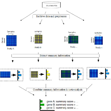
3.1.1 Integration at the Interpretative Level ... 40
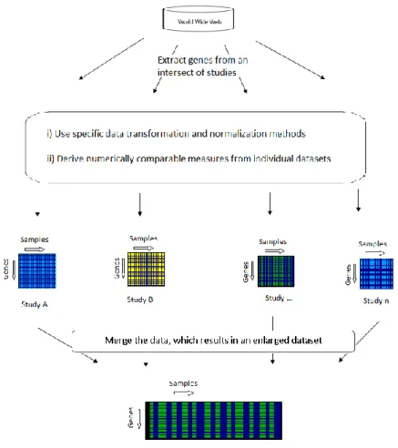
3.1.2 Integration with Rescaling of the Expression Values ... 45
Chapter 4 Data Assessment and Normalization ... 49
4.1 Data Collection... 49
4.2 Affymetrix Data ... 49
4.2.1 Assessment of Raw Affymetrix Data ... 49
4.2.1.1 Inspection for Hybridization Artefacts... 49
4.2.1.2 MA Plots ... 50
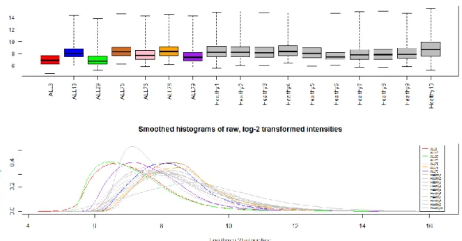
4.2.1.3 Array Intensity Distributions ... 50
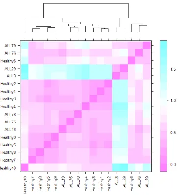
4.2.1.4 Between-Array Comparison... 51 4.2.1.5 GeneChip-Specific Assessments ... 52 4.2.1.5.1 Average Background ... 52 4.2.1.5.2 Scale Factors ... 53 4.2.1.5.3 Detection Calls ... 53 4.2.1.5.4 Hybridisation Controls ... 54
4.2.1.5.5 GAPDH and β-actin Ratios ... 54
4.2.3 Post-Normalization Assessment ... 61
4.2.3.1 MA Plots ... 61
4.2.3.2 Array Intensity Distributions ... 61
4.2.3.3 Normalized Unscaled Standard Error (NUSE) Plot ... 61
4.2.3.4 Between-Array Comparison... 63
4.3 cDNA Data ... 64
4.3.1 Assessment of Raw cDNA Data ... 64
4.3.1.1 MA Plots ... 64
4.3.1.2 Array Intensity Distributions ... 65
4.3.1.3 Between-Array Comparison... 66
4.3.2 cDNA Data Normalization ... 67
4.3.3 Between-Array Normalization ... 70
4.3.4 Post-Normalization Assessment ... 72
4.3.4.1 MA Plots ... 72
4.3.4.2 Array Intensity Distributions ... 72
4.3.4.3 Between-Array Comparison... 72
Chapter 5 Transformation of Expression Data ... 74
5.1 Finding Differentially Expressed Genes ... 74
5.2 Ratio-Transformation ... 80
5.3 Method Validation and Evaluation ... 83
Chapter 6 Formation of a Crossover ... 88
6.1 Modelling the data... 89
6.1.1 Linear model ... 89
6.1.1.1 Linear regression ... 89
6.1.2 Consideration for non-linear models ... 92
6.1.2.1 F-test using ANOVA ... 92
6.1.2.2 Akaike‘s Information Criterion ... 94
6.1.3 Non-linear models ... 95
6.1.3.1 Polynomial regression ... 95
6.1.3.2 Locally weighted regression ... 97
6.1.3.3 Bootstrap Aggregating ... 100
6.1.3.4 Self-Organizing Maps ... 105
6.1.3.5 Feedforward Neural Network ... 111
6.2 Summary of results ... 115
Chapter 7 Closing Remarks ... 117
7.1 Summary ... 117
7.2 Conclusions ... 118
7.3 Advantages and Limitations ... 118
7.4 The Road Ahead ... 120
7.5 Final Remarks ... 120
A.2 MA Plots of Raw Affymetrix Arrays ... 135
A.3 MA Plots of Normalized Affymetrix Arrays ... 136
Appendix B Assessment of cDNA Arrays ... 137
B.1 MA Plots of Untreated cDNA arrays ... 137
Table 2.1 Significance of the spot-colours ... 11
Table 2.2 Gene expression matrix... 23
Table 2.3 List of major noise sources ... 28
Table 4.1 cDNA array-numbers corresponding to the names ... 67
Table 6.1 Linear regression ... 91
Table 6.2 Cubic polynomial ... 95
Table 6.3 Bootstrap aggregating ... 104
Table 6.4 Output of self-organizing maps ... 110
Table 6.5 Results from feedforward network ... 114
Figure 1.1 Microarray technology requires interdisciplinary knowledge ... 2
Figure 2.1 Formation of proteins from genes ... 6
Figure 2.2 Spotting in cDNA microarrays ... 9
Figure 2.3 Overview of a typical spotted microarray experiment ... 10
Figure 2.4 Scanned cDNA image ... 11
Figure 2.5 The principle behind Affymetrix technology ... 13
Figure 2.6 A theoretical account of the fate of a microarray image ... 14
Figure 2.7 Typical cDNA (left) and Affymetrix image (right) ... 14
Figure 2.8 Aligning a grid for identification of each spot ... 15
Figure 2.9 A microarray slide and a spot ... 16
Figure 2.10 Affymetrix data files ... 18
Figure 2.11 Stem cell maturing into different blood types... 33
Figure 2.12 Types of leukaemia ... 35
Figure 3.1 Microarray data integration at interpretative level... 44
Figure 3.2 Microarray data integration with rescaling of expression values ... 48
Figure 4.1 Intensity distributions of raw, log2-transformed Affymetrix arrays ... 51
Figure 4.2 Heatmap for between-array distances for raw Affymetrix arrays ... 52
Figure 4.3 β-Actin and GAPDH (3′:5′ ratios) ... 55
Figure 4.4 β-Actin and GAPDH (3′: mid-ratios) ... 56
Figure 4.5 RNA degradation plot ... 57
Figure 4.6 RLE (Relative Log Expression) plot... 58
Figure 4.7 Boxplots and smoothed histograms of RMA normalized intensities... 61
Figure 4.8 NUSE (Normalized Unscaled Standard Error) plot ... 63
Figure 4.9 Heatmap of normalized Affymetrix data ... 64
Figure 4.10 Untreated expression measures of green and red channels ... 66
Figure 4.11 Heatmap of distances between the raw cDNA arrays ... 66
Figure 4.12 Effect of background-correction on red and green channels ... 68
Figure 4.13 Printtiploess normalization on cDNA arrays ... 70
Figure 4.14 M-value distribution before between-array normalization ... 71
Figure 4.15 M-value distribution after between-array normalization ... 71
Figure 4.16 Post-normalization density estimates of cDNA arrays ... 72
Figure 4.17 Post-normalization heatmap of cDNA arrays ... 73
Figure 5.1 CV as a function of average gene expression across Affymetrix arrays ... 76
Figure 5.2 Linear and logarithmic CV-values with filtering cut-off ... 77
Figure 5.3 Distribution of raw and adjusted p-values ... 78
Figure 5.4 MA-plot comparing healthy and leukaemic samples... 79
Figure 5.5 Volcano-plot of the comparison between healthy and diseased samples ... 79
Figure 5.6 Scatterplot of significant genes from 7-patients ... 80
Figure 5.7 Array distribution before and after ratio-transformation ... 83
Figure 5.8 Hierarchical gene clustering of Affyoriginal (left) and Affyratio (right) ... 84
Figure 5.9 Hierarchical patient clustering of Affyoriginal (left) and Affyratio (right) ... 84
Figure 6.1 Scatterplot of individual patient‘s data ... 90
Figure 6.2 Overlaying of linear fits for each patient ... 90
Figure 6.3 Microarray data with linear, polynomial and loess fit ... 100
Figure 6.4 A schematic of bootstrapping process ... 101
Figure 6.5 Self Organizing Map (1D and 2D)... 106
Figure 6.6 Self-organizing map ... 108
Figure 6.7 Final neuron-positions along with training- and test-data ... 109
Figure 6.8 A model of a neuron ... 112
Introduction
The new millennium is currently witnessing a high-paced information revolution that was initiated in the latter part of the 20th century. This has gifted the common people to realise that the dreams that were seemed distant not a too long ago are indeed possible to see under the broad daylight. Computer technology and internet have catalysed and continually been adding a fuel to this ongoing renaissance. With regards to the promise of our better health through its huge impact on the bioscientific, bioengineering and medical fields, the pair has ushered Bioinformatics, ‗the combination of biology and information technology, dealing with the computer-based analysis of large biological data sets‘ (Fogel & Corne, 2003). The applications of bioinformatics in gene expression profiling help disease diagnosis, prognosis, and therapy. Particularly, microarray-based methods are conferring the freedom to conduct large-scale gene expression profiling measurements; and in conjunction with bioinformatics, it has unleashed a wealth of powerful and previously unattainable prognostic information on cell growth and survival. This availability, versatility as well as integration of new technologies have eliminated many previously existing obstacles and boundaries to march towards unravelling the complex mechanisms hidden beneath complex diseases and networks that regulate gene expression.
The methods to measure gene expression were revolutionized by Kary Banks Mullis‘s invention of the in vitro technique, polymerase chain reaction (PCR) in 1985 that awarded him Nobel prize for Chemistry in 1993. PCR (Mullis et al., 1986; Saiki et al., 1985) exponentially amplifies and synthesises new DNA molecules via enzymatic replication. While the variants of PCR, such as RT-PCR (reverse transcription polymerase chain reaction) or Q-PCR (real time quantitative polymerase chain reaction, or qrt-Q-PCR) can detect the expression of one gene within one reaction or to a maximum of a few genes in optimised state, high-throughput analysis of higher number of genes is very time consuming, and requires a lot of technical and personal power. In 1995, two seminal publications, namely Schena et al. (1995) and Smith et al. (1995), led by investigator, Patric O. Brown of the Howard Hughes Medical Institute and his colleagues, launched the era of low cost gene-expression microarray analysis. From 1995, the technique of microarrays, which started off with simultaneous gene expression analysis of 45 genes within one experiment, has been improved dramatically and has become a widely used tool for studying global gene expression of cells in culture or
paradigm of studying ‗one gene at a time‘, and provided technological and conceptual advancement through its high-throughput capability of simultaneously interrogating the RNA expression of the whole genomes on a single chip. From the late nineties, researchers have started conducting microarray experiments using either of the two distinct techniques - cDNA-microarrays and Oligonucleotide cDNA-microarrays. With the development of this field, different labs have begun to routinely fabricate customized arrays.
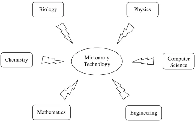
As gene expression microarrays gradually became widely applied for addressing increasingly complex biological questions, an unprecedented amount of data have started been generated. This catalyzes contributions from various interdisciplinary fields, which constitute integral components of the technology. The knowledge of different fields soon becomes a necessity while studying microarray technology, as depicted in Figure 1.1. It has also liberated the researchers to employ microarray technology in a much wider range of applications, including experimental annotation of the human genome, discovery of gene functions, analysis of complex diseases, biological-pathway dissection, tumour profiling, diagnostic and prognostic predictions for various cancers, drug-target identification and validation, biomarker identification, and compound-toxicity studies (Imbeaud & Auffray, 2005).
Figure 1.1 Microarray technology requires interdisciplinary knowledge Microarray Technology Biology Chemistry Physics Mathematics Computer Science Engineering
Over a short time, microarray technology has indeed positioned itself in the scientific world as a reliable approach for gene expression analysis. There are, however, still issues that are not yet unanimously resolved, such as reliability and reproducibility (S Draghici, Khatri, Eklund, & Szallasi, 2006; P. J. Park et al., 2004), experimental design (Yee Hwa Yang & Speed, 2002), statistical issues (Nadon & Shoemaker, 2002; Gordon K. Smyth, Yang, & Speed, 2003), image processing (Jouenne, 2001), and others (Imbeaud & Auffray, 2005; Murphy, 2002; P. J. Park et al., 2004). One such critically unresolved niche of microarray technology lies in the integration of data from different microarray experiments.
The freedom of having multiple platforms to conduct microarray investigations as well as the ever increasing number and publicly available gene expression studies of human and other organisms provide the researchers with strong motivations to carry out cross-study analyses. Integration of multiple microarray experiments carries enormous potential towards obtaining higher accuracy, consistency and robust information mining. Moreover, the integrated results can help in constructing a broader picture crystallizing the biological mechanisms.
The goal intended to be attained in this research work remains within the vicinity of intersection of two specific platforms - cDNA (or, spotted arrays) and Affymetrix®. Firstly, a novel approach is to be designed and implemented that integrates the data from the two platforms. This method is then required to be validated as well as evaluated to examine where it stands in the midst of methods available from microarray literature. Further, investigation needs to be carried out with the merged data towards analysing whether there is any association between the two platforms; and if the answer is positive, then carry out investigations and find out how best this association could be defined.
The overall thesis, including this introductory segment, is comprised of seven chapters. A glimpse of the layout follows.
Chapter 2: Microarray Technology and Cancer
The 2nd chapter provides a broad overview of microarray technology. Starting with an introductory overview, it explains the various microarray types and the process of microarray data analysis along with the challenges and applications of the technology. The chapter also highlights the fact that cancer has become a perfect candidate for evaluation by microarray technology, being the disease both dreadful and challenging because of its polygenic nature. It appraises the application of microarray technology in cancer research. Besides, this chapter
provides an overview of this disease in general, and leukaemia in particular as the data used in this project belong to a group of childhood leukemia patients.
Chapter 3: Microarray Data Integration: A Review
Integration of data from different microarray experiments is a challenging problem. This chapter carries out a review on several important experiments conducted and published with regards to microarray data integration.
Chapter 4: Data Assessment and Normalization
Assessing the quality of data is critical prior to carrying out any analytical investigations. This chapter begins with introducing the data, which would be used for carrying out the investigations, and then conducts an elaborate assessment of the quality of these data.
Normalization is a transformation method applied to expression data that appropriately adjusts the individual hybridization intensities so that meaningful biological comparisons can be made. After data quality assessment, the focus remains on the application of normalization on the datasets along with the effects. Finally, the chapter conducts a post-normalization quality check on the data.
Chapter 5: Transformation of Expression Data
Microarray experiments are often conducted using two of the most commonly used platforms - Affymetrix® and spotted arrays. However, there is always an issue of incomparability between the expression data from these two microarray platforms. This chapter attempts to address this issue by structuring a new approach, which is subsequently validated as well as evaluated.
Chapter 6: Formation of a Crossover
The 6th chapter explores in the direction of seeking an association between the two platforms, Affymetrix and spotted arrays. In this regard, a wide range of statistical and machine learning approaches are applied to the microarray data to probe into this possibility. Finally, the chapter compares all the methods, and highlights the ones that stand out in this investigation.
Chapter 7: Closing Remarks
This chapter presents the concluding segment of the thesis that contains the final remarks on the work including the advantages and limitations, and potential lines of future investigations.
References
Chapter 2
Microarray Technology and Cancer
2.1 Microarray Technology
2.1.1 Microarrays – An Overview
All living organisms contain DNA, a molecule that holds all the information required for development and functioning of any organism. Deoxyribo nucleic acid, or DNA encodes for genes, and through the process of gene expression, the information from a gene is used in the synthesis of a functional gene product - either protein or RNA. The process usually starts in the nucleus of a cell when the genetic information of DNA flows to messenger RNA (mRNA) by a process called transcription. The mRNA then goes out of the nucleus to the cytoplasm of the cell, and interacts with ribosome, a specialized complex. Ribosome decodes the information to amino acids, the building blocks of proteins, through another process known as translation. A type of RNA called transfer RNA (tRNA) assembles the protein, one amino acid at a time. This flow of information from DNA to RNA to proteins is so fundamentally important in molecular biology that it is called the central dogma. A portrayal of the process, as given by US National Library of Medicine, is in Figure 2.1. In brief, this process of turning the genetic information present in the DNA into proteins is known as gene expression.
Figure 2.1 Formation of proteins from genes
The human body contains different types of cells, and all the cells contain the same DNA. However, each type of cell expresses a unique configuration of genes. This is assured by the
control of the regulatory elements, which switch the genes to either on- or off- state. Microarrays are a tool used to record such states of DNA.
Microarrays provide a way to gain information on the deepest biological mysteries encoded in the informationally complex DNA. Cellular DNA is structurally helical often with two antiparallel strands made up of a combination of four nucleotides, or bases: adenine, cytosine, guanosine, and thymidine (abbreviated respectively as A, C, G, or T). The nucleotides are covalently linked to a sugar phosphate backbone of each strand. According to a set of pairing rules, the nucleotides of one strand remain hydrogen-bonded with the nucleotides of the other strand. For the cells to express genes, the strands are opened by gene expression machinery so that complementary RNA-copies of a gene can be synthesised. Two complementary single-stranded nucleic acid molecules tend to come together and reanneal to form a double helix complex (Marmur & Doty, 1961). Two single-stranded nucleic acid molecules that are not fully complementary can also bind, but as the complementarity increases, the binding becomes stronger. Overall, this binding process is called hybridization. Hybridization is at the centre of many biological as well as in vitro analytical processes. Even if molecules come from different sources, they will hybridize if they match.
Hybridization-based approaches have been used for decades to measure nucleic acid sequences (Amos, 2005). Developed at Stanford University, northern blot technique (Alwine, Kemp, & Stark, 1977) is the most widely accepted standard for hybridization-based assay of gene expression where the size and abundance of RNA transcribed from a gene is measured. Microarrays are developed from blotting assays, the techniques that are used in molecular biology and clinical research to identify unique nucleic acid (or, protein) sequences in a highly specific and sensitive way (Hayes, Wolf, & Hayes, 1989).
In a microarray framework, there is a substrate, or an array made of nylon membrane, plastic or glass on which various fragments of single stranded DNA, or ssDNA are attached in localised features while arranging in regular grid-like pattern. The substrate is then used to answer a specific query regarding the ssDNA on its surface. The term, probe is used to refer the ssDNA. The target is a solution of ssDNA that is applied for hybridization with the probes on the substrate. This hybridization between the targets and the probes on the surface of the substrate is essential to conduct the required interrogation. During the hybridization process, the target formes heteroduplexes1 via base-pairing with the probes. Subsequently, as the
hybridization completes, the amount of gene expression is computed, probed into and quantified.
2.1.2 Microarray Types
There are mainly two commonly used microarrays that fall into a broader category known as
nucleic acid microarrays: cDNA microarrays and Oligonucleotide microarrays. Each
effectively serves as a genomic readout while possessing unique characteristics along with advantages as well as disadvantages in a given context.
2.1.2.1 Spotted Microarrays
Spotted, or cDNA microarrayswere the first available platform that originated in Pat Brown‘s
laboratory, and continue to enjoy broad application. These are primarily a comparative technology where relative concentrations between two samples are examined.
In spotted microarrays, the probes are either libraries of PCR (polymerase chain reaction) products that correspond to mRNAs, cDNAs2 or oligonucleotides3. Once synthesised, these are transferred to the substrate, usually glass microscope slide. The probes are printed in an orderly manner at specific locations called spots or, features using a robot equipped with nibs capable of wicking up DNA from microtiter plates and depositing it onto the glass surface with micron precision (M Schena et al., 1995). Babu (2004) explains it with a schematic, which is given in Figure 2.2.
Samples to be compared are labelled with uniquely coloured fluorescent tags before being mixed together. The fluorescent labelling is done with the fluorophores Cy3 and Cy5, represented by the pseudo-colours green and red respectively, using either of the two common approaches – direct or indirect labelling. In direct fluorescent labelling, the fluorescent tags are attached in a covalent manner to the target molecules using enzymatic or chemical means, while in indirect labelling, the tags are attached in a non-covalent and indirect way to the target molecules using dendrimers, antibodies or other reagent (Mark Schena, 2003). Some investigators believe that all arrays should be performed both forward- and reverse labelled. That is, for an array with sample A labelled with Cy3 and sample B with Cy5, there should be another array where sample A is labelled with Cy5 and sample B with Cy3. However, Dobbin and his colleagues (Kevin Dobbin, Joanna H. Shih, & Richard Simon, 2003; K. Dobbin, J. H. Shih, & R. Simon, 2003) recommend against this reverse labelling, also known as dye-swap.
2 mRNA is very unstable outside of a cell, and converted in the laboratory to complementary DNA (cDNA), which only contains expressed DNA sequences, or exons. In the process, often incomplete sequences, called expressed sequence tags (ESTs) result from each mRNA molecule due to certain technical aspects.
Figure 2.2 Spotting in cDNA microarrays
The labelled cDNAs are allowed to hybridize with the probes on the substrate under stringent conditions. Hybridization process continues for several hours, which provides a way of comparing the relative differences between the two samples on a per spot basis depending on the fractional occupancy of the spot hybridized by each sample. At the end of hybridization, excess of the labelled samples is removed by washing, and the slide is dried. Laser scanning is the next and final experimental stage. Here, the slide is excited using a laser at different wavelengths, one for each of the fluorophores used, and the respective fluorescence is
captured as two independent, 16-bit, black-and-white TIFF4 images (Causton, Quackenbush,
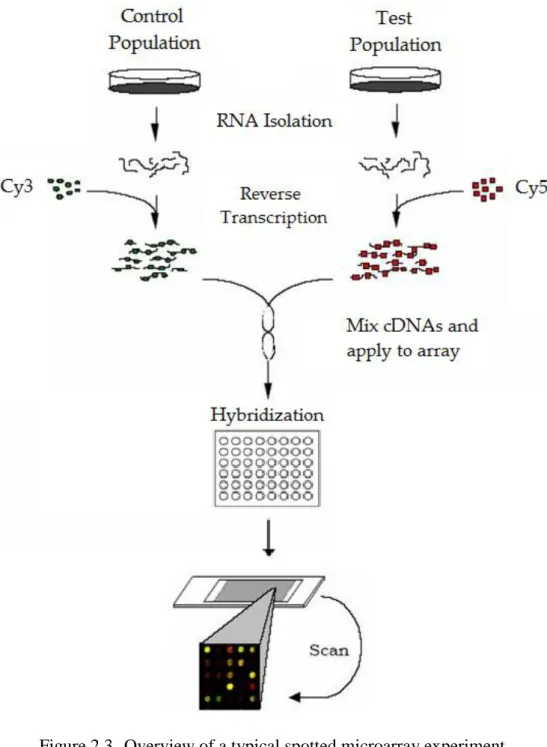
& Brazma, 2003). The intensity of each spot on these two images is theoretically proportional to the amount of mRNA transcripts of the query (or, test) and control (or, reference) sample. Image recognition software processes the two images, and produces the gene expression levels by converting the gene expression pixel-level intensities into numeric values. An overview5 of a typical experiment is provided in Figure 2.3.
Figure 2.3 Overview of a typical spotted microarray experiment
For the purpose of visually displaying the information, both the images of raw intensities are compressed into 8-bit images, using a square root transformation, from which the image processing software creates a composite image (usually 24 bit) that exhibits artificial florescence colours for Cy3- and Cy5- channels ranging from green through yellow to red for the spots (Y. H. Yang, Buckley, & Speed, 2001). Therefore, in the absence of dye-swap, the decisions or comments can be made based on the spot-colours: a) Red spot: genes prevalently expressed (upregulated) in the tumour sample; b) Green spot: genes prevalently expressed in the normal sample (downregulated in tumour); c) Yellow spot: Genes equally expressed in both normal and tumour tissue; d) Black spot: Genes not detected in any of the samples. This is summarised in Table 2.1, and is also shown in Figure 2.4.
Table 2.1 Significance of the spot-colours
Spot color Signal strength Gene expression
Yellow Healthy = Diseased Unchanged
Red Healthy < Diseased Induced
Green Healthy > Diseased Repressed
Black Unknown/no expression Unknown/no expression
Figure 2.4 Scanned cDNA image
2.1.2.2 Oligonucletide Arrays
Oligonucleotide arrays are fundamentally different from spotted arrays. Unlike cDNA arrays
which can use long DNA sequences, oligo arrays can ensure the required precision only for short sequences. Therefore, these arrays represent a gene using several short ssDNA sequences, called oligonucleotides, or oligos. Three approaches represent the in-situ process of microarray fabrication:
The photolithographic approach is based on the same technique as used in the
semi-conductor industry to make the microprocessors. Affymetrix Inc. (Santa Clara, California) has commercialised the photolithographic method, pioneered by Fodor et
GeneChips are the probe-holding devices, and are also generally referred to as biochips. At Affymetrix, GeneChips are manufactured by a proprietary, light-directed chemical synthesis process, which combines solid-phase chemical synthesis with photolithographic fabrication techniques.
The ink jet approach employs the technology used in the ink jet colour printers. Nucleotides (A, T, G and C) are loaded in the four cartridges. As the print head with the cartridges moves over the array-substrate, specific nucleotides are deposited where
required. Several companies such as Protogene (Menlo Park, CA) and Agilent
Technologies (Palo Alto, CA) in collaboration with Rosetta Inpharmatics (Kirkland, WA) have developed methods of in situ synthesis of oligonucleotides on glass arrays using ink jet technology.
The electrochemical synthesis approach is introduced by CombiMatrix Corporation6
(Washington, USA). The process uses small electrodes embedded into the substrate. After solutions containing specific bases are washed over the substrate, electrodes are activated on required positions in a predetermined sequence allowing them to be constructed base-by-base.
Here, the focus would remain on Affymetrix GeneChips, which are the most ubiquitous and long-standing commercial microarray platform in use (Seidel, 2008).
Affymetrix represents a gene through multiple probe-pairs which are contained in a silicon chip, GeneChip. Typically 16–20 of these probe-pairs, each interrogating a different part of the sequence for a gene, make up what is also known as a probeset; and some more recent arrays, such as the HG-U133 arrays, use as few as 11 probes in a probeset (B. M. Bolstad, Irizarry, Astrand, & Speed, 2003). The size of a standard GeneChip is 1.28 cm × 1.28 cm; and over 6.5 million squares, or features are present on each chip. In each feature, there are millions of identical probes. The design of Affymetrix probes is not usually in the hands of the researchers. A probe consists of a short oligonucleotide sequence containing 25 nucleotides, called a 25-mer; and all the probes are synthesised on the chip one base at a time, and in parallel at all locations. A paired probe is composed of: a) a perfect match (PM), which is the exact sequence of the chosen fragment of the gene, b) a mismatch (MM), which is same as PM but contains a mismatch nucleotide in the middle of the fragment. Affymetrix anticipates that the MM probe does not hybridize well to the target transcript, but hybridizes to many transcripts to which the PM probe cross-hybridizes (Simon et al., 2004). Therefore,
the intensity difference between PM and MM paired probe is considered to be a better estimate of the hybridization intensity to the true target transcript.
A single sample is usually hybridized to GeneChips. For using as target, the total mature, spliced, poly-A tail added RNA isolated from the cell being studied is turned into a double stranded cDNA through reverse transcription. At the time of running the array, the cDNA is allowed to go through in vitro transcription back to RNA (now known as cRNA), and labelled with biotin. The labelled cRNA is then randomly fragmented in to pieces anywhere from 20 to 400 nucleotides in length, and the cRNA fragments are added to GeneChip for hybridization.
The hybridization occurs at a critical temperature. After hybridization, the difference in hybridization signals between PM and MM, as well as their intensity ratios, detected by scanning the array with a laser serves as indicators of specific target abundance. The value that is usually taken as representative for each gene‘s expression level is the average difference between PM and MM. Ideally, this average value is expected to be positive because the hybridization of the PM is expected to be stronger than the hybridization of the MM. However, many factors, including non-specific hybridizations and a less than optimal choice of the oligonucleotide sequences representative of the gene, might result in an MM hybridization stronger than the PM hybridization for certain probes. The calculated average difference might be negative in such cases, and these negative values introduce noise into the dataset. The overall principle behind Affymetrix technology is summarised in Figure 2.5 (S. Draghici, 2002).
Figure 2.5 The principle behind Affymetrix technology
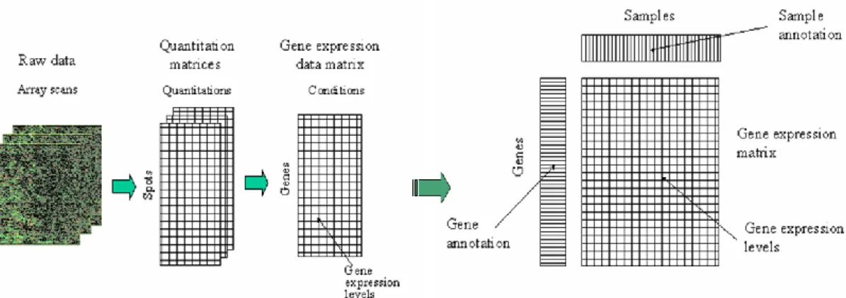
The expression data from both types of microarrays are finally obtained in the form of a matrix with genes as rows and conditions as columns, and subsequently biologically
meaningful information is extracted and added. Accordingly, Figure 2.6 presents the final fate of a microarray image7.
Figure 2.6 A theoretical account of the fate of a microarray image
2.1.3 Processing of Array Output
The outputs of microarray experiments require processing before they can be used for extracting meaningful information. Image processing and normalization are the two preliminary microarray data processing stages.
2.1.3.1 Image Processing
Regardless of the technology, the arrays are scanned after hybridization and independent, 16 bit, digital, grey-scale TIFF images are generated for query and control samples (Causton et al., 2003). Figure 2.7 presents two typical pseudo-coloured images from Affymetrix and cDNA platforms. The process of image processing for the two platforms is different, and is briefly given below.
Figure 2.7 Typical cDNA (left) and Affymetrix image (right)
2.1.3.1.1 Image of cDNA Microarrays
Analysis of a cDNA image seeks to extract intensity for each spot or feature on the array, and it involves various image processing stages that can be carried out through different microarray image analysis software. The analysis is done mainly using the following steps –
A. Gridding.
This is usually a semi or fully-automated measure based on Bayesian statistics to locate each spot on the slide. In the process of gridding, a grid is placed over the hybrid compound fluorescence in the image so that each fluorescence is contained within a patch. This is shown in the image8 of Figure 2.8.
Figure 2.8 Aligning a grid for identification of each spot
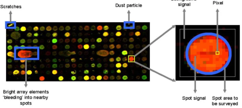
B. Segmentation.
A microarray spot contains two components – signal and background. Signal corresponds to the true intensity values of the foreground, and the background, or noise is the unwanted intensity values associated with events like spurious biochemical processes and substrate reflection. It is depicted in the image9 of Figure 2.9. Once the signals are identified, they need to be separated from the background. Segmentation performs the task of partitioning the image into foreground (spot) and background.
Figure 2.9 A microarray slide and a spot
Several algorithms are in use for segmentation process. Yang et al. (2002) categorises the various existing segmentation schemes into four groups: (1) fixed circle segmentation, (2) adaptive circle segmentation, (3) adaptive shape segmentation, and (4) histogram segmentation.
Fixed Circle Segmentation sets a round region of constant diameter in the middle of each spot as the target site, and is provided in most existing software packages including
ScanAlyze10, GenePix (Axon Instruments, Redwood City, CA) and QuantArray (GSI
Lumonics, Inc., Watertown, MA). This is the most straightforward method which assumes that all spots are circular with constant diameter, and everything inside the circle is the signal and everything outside is the background. But this assumption rarely holds, and so most
image analysis software includes some more advanced segmentation methods. Adaptive circle
segmentation, used by tools like GenePix and Dapple11(Buhler, Ideker, & Haynor, 2000), estimates circle diameter separately for each spot. The circular spot signals are quite rare, and therefore, adaptive shape segmentation tries to find the best shape to describe a spot.
Histogram method, used by tools like ImaGene (BioDiscovery, Inc., Los Angeles, CA) and QuantArray, analyses the signal distribution in and around each spot to determine which pixels belong to the spot and which pixels belong to the background.
C. Foreground Intensity Extraction and Background Correction.
Once the spot and background areas are defined, each pixel within the area is taken into account; and, the mean, median, and total value of the intensity over all the pixels in the defined area are reported for both the spot and background. The signal and background intensity is computed in several different ways, the most common being the mean and the
10 Available at: http://rana.lbl.gov/EisenSoftware.htm 11 Available at: http://www.cs.wustl.edu/~jbuhler/dapple/
median. Background subtraction is the process where the intensity corresponding to the background is subtracted from the spot intensity to obtain more accurate quantitation representing a spot.
D. Expression Ratio and its Transformation.
The relative expression level for a gene can be measured as the amount of red or green light emitted after laser excitation. The common measurement used to relate this information is called Expression Ratio, Tk, which is denoted by:
where for each gene k on the array, Rk and Gk represent the spot intensity metric for the tumour sample and the healthy sample, respectively. The spot intensity metric for each gene can be represented as a total intensity value or a background subtracted median value.
It is common practice to transform the raw counts into a different scale that is more convenient and statistically sound. There are two kinds of transformation reported for the expression ratio - inverse transformation and logarithmic transformation. The latter takes the logarithm base 2 value of the expression ratio [i.e., log2 (expression ratio)]. It is considered a better transformation procedure because it treats differential up-regulation and down-regulation equally, makes the distribution more symmetrical and the variation less dependent on absolute signal magnitude (Babu, 2004; Simon et al., 2004). The log2–ratio for each spot can be written as given in equation 2, where RForeground and GForeground represents the foreground (the patch of a spot) mean or median intensities of red and green channels, and RBackground and GBackground denotes the corresponding background mean or median intensities.
2.1.3.1.2 Image of Affymetrix GeneChipTM
Affymetrix has integrated its image processing algorithms into the experimental process of
Background Foreground Background Foreground G G R R 2 log ( 2 ) Tk = k k G R ( 1 )
Affymetrix GeneChip experiments are managed with the Affymetrix GeneChip Operating
Software (GCOS) or Affymetrix Microarray Suite (MAS). Once the fluorescent-tagged
nucleic acid sample is injected into the hybridization chamber, and hybridization takes place to the complementary oglionucleotides on the chip, the hybridized chip is scanned and the laser excited fluorescence across the chip is converted to a 2D image. This image data file (.DAT) can be exported as a .TIFF image. The image data file is used by the software to generate a .CEL file that gives the position and intensity information of each probe for one GeneChip, in addition to the position of masks and outliers.
The Affymetrix output result file is the .CHP file, where the average signal intensities are linked to gene identities. The report file (.RPT) is generated from the .chip file, and it summarizes the quality control information about expression analysis settings and probe set hybridization intensity data. Besides, there are two more files that are used in the actual analysis process - Experiment File (.EXP) and Chip Description file (.CDF). The former contains parameters of the experiment such as probe array type, experiment name, equipment parameters and sample description. The .CDF file is provided by Affymetrix and describes the layout of the chip. According to the overall Affymetrix file types summarised in Figure 2.10, the .DAT files are analysed and the intensity data, thus generated, are saved as .CEL files. The .TXT file is a .CHP file in text format.
Figure 2.10 Affymetrix data files
A typical Affymetrix probe set contains 11 perfect match probes and 11 mismatch probes. Although Affymetrix has a standard method for summarizing 22 readouts to obtain a single number for gene expression (Affymetrix, 2002), many approaches are available (Rafael A. Irizarry, Wu, & Jaffee, 2006). Usually, the final expression of a gene is the average difference between all the PM and MM probes of a gene, and is considered proportional to the actual expression level of the gene. It is given in equation 3, where n represents the total number of probe pairs for the gene, and PMi and MMi indicate the corresponding PM and MM probe intensities after background correction for the ith probe pair of the gene.
2.1.3.2 Data Normalisation
Data normalisation is an important aspect, and plays an important role in the early stage of microarray data analysis as the subsequent analytical results are very much dependent on it. The normalization methods rely on the fact that gene expression data can follow a normal distribution, and the entire distribution can be transformed about the population mean and median without affecting the standard deviation. The objective of normalization is to eliminate the measurement variations and measurement errors, and to allow appropriate comparison of data obtained from the expression levels of genes so that the genes that are not really differentially expressed have similar values across the arrays. Normalization is also used to identify and eliminate questionable and low quality data.
Normalization approaches typically use either a control set of genes or the entire genes from an array. The use of a control set requires only one assumption, i.e., the control genes are detected at constant levels in all of the samples being compared.
Housekeeping genes constitute a type of control gene set, and are considered to be used in normalization as they are expressed in most, if not all cells. As the cells need these genes for cell maintenance and survival, such genes are expected to be similarly expressed in all samples of experiment. However, it is difficult to identify these genes as the genes regarded to be housekeeping for one tissue type may not be the same for another type of tissue. To ensure that a gene can be considered as a housekeeping gene, carefully controlled experiments are performed. A number of techniques are used to identify housekeeping genes based on the observed data, such as the rank invariant selection method of Schadt et al. (2001), and the iterative method of Wang et al. (2002). For GeneChips, Affymetrix Inc. claims to have integrated the housekeeping genes in the chips after supposedly testing them on a large number of various tissue types with the resultant low variability in those samples.
Spiked-ins, or spiked controls, are another set of control genes, which are exogenous RNA added proportionately to both query and reference samples, otherwise not found in either sample. The need of these exogenous control genes arises as there is accumulating evidence to
Differenceprobepair PMi – MMi
( 3 ) ) ( 1 i i i pair probe PM MM n difference Average
suggest that many housekeeping genes change in expression under some circumstances (P. D. Lee, Sladek, Greenwood, & Hudson, 2002; Thellin et al., 1999).
Besides, there is one more alternative for selecting a dataset for applying normalization. It is to order the genes or signal from each spot based on expression level, and using only those within a fixed window centred within the dataset (e.g., those between the 30th and 70th percentile) or those within a fixed number of standard deviations of the mean (Eric E. Schadt, Cheng Li, Byron Ellis, & Wing H. Wong, 2001; Tseng, Oh, Rohlin, Liao, & Wong, 2001). Once a gene set for normalization is selected, normalization process can be conducted.
2.1.3.2.1 cDNA Normalization
For cDNA microarrays, normalization involves determining the amount by which the genes of the red channel are over- or under expressed relative to the green channel. This bias is known as normalization factor or scaling factor, and is different for different arrays. The normalisation factor, Cjk is subtracted from the log-ratio of the background-corrected red and green signals as shown in the equation 4 below to find the normalised signal intensity, Xjk for a gene, k on array, j. Here, Rjk andGjk represent background-corrected red and green signals, respectively.
Approaches to calculate the normalization factor can be divided into three categories: global normalization, intensity-based normalization and location-based normalization as well as a hybrid of intensity- and location-based normalization.
i) Global, or Linear Normalization.
Global normalization applies the same normalization factor to all the genes on the array, but the value varies from array to array. It assumes that the red and green intensities possess an approximately linear relation. Global normalization uses the global median of log intensity ratios as median is less likely to be influenced by the outliers. Moreover, as it is assumed that the over-expressed proportion of the genes in a given sample is approximately equal to the
jk jk jk jk C G R x log ( 4 )
under-expressed proportion, so by using median, focus remains on those genes which are not differentially expressed in the red and green channels and are expected to be at the centre of the log-ratio distribution.
Global normalization is the simplest and widely used normalization method that works well for most applications including in situations where a relatively small number (example, 50-100) of normalization genes are normalized. The expression can be formulated as below, where S represents the set of normalization genes. Here instead of median, mean can also be used, but it is to be noted that mean is affected by outliers.
ii) Intensity-Based Normalization.
Intensity-based normalization is described in Yang et al. (2002), and it is necessary that there be normalization genes across all intensity values in order to perform this normalization. Again, even if all genes are being used in normalization, there is the implicit assumption that at each intensity level, there are equal numbers of up- and down-regulated genes. However, it is possible that this assumption could be violated, if all the high- (or low-) intensity genes share similar biology. While using intensity-based normalization at intensities for which there are few spots, the normalization could be based on a rather small number of points that may result overfitting to those particular values.
Dudoit et al. (2002) demonstrates a version of representation of intensity whereby a plot becomes more revealing in terms of identifying spot artefacts and detecting intensity dependent patterns in the log ratios. This representation plots log intensity ratio, M( log2 )
G R
on the y-axis against the mean log intensity, A (log2 RG) on the x-axis (R and G represents background adjusted intensity levels for a given spot). This M vs. A plot (MA, or RI plot) shows whether log ratio, M is dependent on the overall spot intensity (which is RNA abundance over all normalization genes), A. In other words, the plot helps to detect intensity dependent patterns in the log-ratios. When it is so found, then it would suggest that an intensity (A) dependent normalization method may be preferable than global methods (such as normalization by the mean or median of M values).
(log jk) jk j k S jk R C C median G ( 5 )
No normalization: The graph-points appears symmetrically scattered around the horizontal line, M=0.
Global normalization: The graph-points appears symmetrically scattered around a
horizontal line, and the line will be shifted up or down, away from M=0 by an amount equal to the required normalization.
Intensity-based normalization: The graph-points follow a line with non-horizontal
slope or a non-linear curve.
Yang et al. (2002) suggest a normalization method for gene expression data that uses smoothing of the MA plot, and this approach is referred to as intensity-based normalization. If intensity-based normalization is decided to apply, a curve is fitted to the MA plot for the normalization genes. Loess curves are more commonly used compared to other smoothing functions. Then, normalization factor, Cjk is defined as in equation 6, where fj is the smoothing function fitted to jth array, and Ajk is the average intensity of gene, k on the jth array.
iii) Location-Based Normalization.
Many times, due to even subtle differences on the degree of wear of the print-tips used to create a slide, the spots on the array vary. Location-based normalization refers to this aspect which deals with normalizing with respect to the print-tip.
Each print-tip generates a grid that is located at a separate place on the array. Yang et al. (2002) suggest performing normalization separately for each print-tip. For normalization within a grid, the same formula is used (i.e., with median) as mentioned under, Global Normalization on page 20.
For location-based normalization, there should be significant numbers of normalization genes within each grid as well as on the entire array, and thus, the method is not applicable to a small number of housekeeping or spiked control genes. Moreover, to account for all location effects, estimation methods based on several parameters exist which look beyond the print-tip effect.
2
( ) (log )
jk j jk j jk jk
iv) Merging of Location and Intensity Normalization.
It is possible to combine both location- and intensity-based normalizations for better results. Two possible actions can be taken in this regard. One option is to apply global normalization to each grid of the array and then, to apply intensity-based normalization to the entire array. According to Yang et al. (2002), a better alternative is to use intensity-based normalization separately within each grid. However, it is not suitable at intensities where the data are sparse. After normalization the processed data can be represented in the form of a matrix, gene expression matrix. Babu (2004) shows it figuratively as in Table 2.2, where each row corresponds to a particular gene, and each column either corresponds to an experimental condition or a specific time point at which expression of the genes has been measured. The expression levels of a gene across different experimental conditions are together termed as the gene expression profile, while that of all genes under an experimental condition are together termed as the sample expression profile.
Table 2.2 Gene expression matrix
[A: The value of each matrix-cell, in arbitrary units, reflects the expression level of a gene under a condition. B: Condition C4 is used as a reference and expression ratios are obtained by normalizing all other conditions with
respect to C4. C: In this table, all expression ratios were converted into the log2 values. D: Discrete values for the
elements in C are obtained by converting log2 values > 1 to 1, < –1 to –1, and a value between –1 and 1 to 0. (Babu,
2.1.3.2.2 Normalization of Affymetrix Arrays
Affymetrix GeneChip arrays have single channel (and colour), and use the same
normalization methods for all the arrays, unlike the two-colour cDNA microarrays. Location-based normalization is not used for these arrays as location-specific intensity imbalances, even if they may appear, are less severe having smaller degree of impact on the mean differences of the individual genes. Normalization of Affymetrix arrays is done mainly to account for variations associated with technological reasons. Like cDNA microarrays, normalization factor should be calculated separately for these arrays too.
i) Global or Linear Normalization.
It is a straight-forward method of normalisation, as used in cDNA microarrays, where one normalization factor is used for all the genes on the array. Affymetrix makes use of average intensity (different from cell average intensity) of an array which is defined as the mean of all the average difference values except the lowest and highest 2% of the data which is not included in the averaging calculation. The idea of this procedure is to find the normalization factor by making the average intensity of the experimental array numerically equivalent to the average intensity of the baseline array12, as given in equation 7.
ii) Intensity Based Normalization.
Like cDNA arrays, MA plots can also be generated for GeneChiparrays to determine whether
intensity-based normalisation is required. In such a plot, a pair of arrays is compared, prior to which a choice needs to be made as to which array to normalize against. If Xk and Yk denote the normalised signal log value for gene k on two arrays, X and Y, respectively, then M vs. A can be plotted based on equation 8.
12 Baseline Array: An array designated as the baseline when used in comparison analysis with which the experimental array is compared to detect changes in expression.
Mk = Xk - Yk ( 8 ) Ak= ( ) 2 1 k k Y X 1 1 , 96 n jk kj kj k C PM MM n k S S percentile
( 7 )The result of MA plots can be interpreted as follows:
No normalization: The graph-points appears to be scattered around the horizontal line
at M=0. Many times, this is the case as the genes do not vary considerably from array to array.
Global normalization: The graph-points appear symmetrically scattered around a horizontal line, and the line will be shifted up or down, away from M=0 by an amount equal to the required normalization.
Intensity-based normalization: The graph-points follow a line with non-horizontal slope or a non-linear curve.
There is another method of intensity-based normalization as recommended by Simon et al. (2004). Here, a baseline array is chosen whose scaling factor is closest to the median of the scaling factors of the arrays being analysed. Then MA plots are generated considering the signal for the array being normalised as the query channel and that for the baseline-array as the reference. If MA plot suggests intensity-based normalization, then quantile normalization or loess smoother-based normalisation can be applied using the baseline-array as the reference.
Bolstad et al. (2003), based on a study on the methods of intensity-based normalization of Affymetrix data, recommends quantile normalization method. The method is based on the assumption that the distribution of the expression values does not change dramatically between arrays and that there is a monotone relationship between the gene expression level and probe value within a single array.
Overall, for Affymetrix, there are dozens of methods - as of 2006, more than 30 methods have been identified (Rafael A. Irizarry et al., 2006). Many such methods are popular, namely MAS5 (Affymetrix, 2002), RMA (R. A. Irizarry et al., 2003), GCRMA, dCHIP (C. Li & Wong, 2001), GLA (Zhou & Rocke, 2005); however, no method is clearly the best (Qin et al., 2006).
2.1.4 Applications of Microarrays
The development and use of microarrays are expanding rapidly. It was initially developed for DNA-mapping (Carig, Nizetic, Hoheisel, Zehetner, & Lehrach, 1990) and sequencing-by-hybridization, or SBH (Bains & Smith, 1988; Drmanac, Labat, Brukner, & Crkvenjakov,
1989; Khrapko et al., 1989)applications. Over time, microarray technology has been used in varied applications.
Commonly, microarrays are used in gene expression measurements – ranging from characterizing cells and processes (J. DeRisi et al., 1996; J. L. DeRisi, Iyer, & Brown, 1997; Hughes, Marton et al., 2000) to clinical applications such as tumour classification (Alizadeh et al., 2000; Golub et al., 1999). The technology is also very commonly used in genotyping and the measurement of genetic variation (Magi et al., 2007; Winzeler et al., 1998).
Microarray technology can characterize different molecular complexes of DNA or RNA shedding light on their biological mechanisms. For example, P-bodies are such identified complexes of protein and RNA, which are believed to take part in gene expression by regulating mRNA in the cytoplasm (Parker & Sheth, 2007), and microarrays could be used to monitor and characterize the trafficking of cellular RNA through this complex.
The position of a gene or a DNA sequence on a chromosome is location-specific, and any change in the positions is implicated in tumorigenesis and cancer. Using comparative genomic hybridization, microarrays have been used to examine this as well as aneuploidy13 in a variety of cell types (Pollack et al., 1999; Shadeo & Lam, 2006). As Khodursky et al. (2000) have examined, microarrays can be used to probe into the progress of replication forks, the structure that forms within the nucleus when two DNA strands start separating into two single-stranded DNA during the process of DNA replication. Microarray technology is also used for genome-wide screening of RNA modifying enzymes (Hiley et al., 2005), and increasing our understanding of gene regulatory circuitry (Boyer et al., 2005; T. I. Lee et al., 2002). Hoheisel (2006) and Stears et al. (2003) are two useful reviews that highlights several other useful scientific applications of microarray technology.
There is notable applications of microarray technology in pharmaceutical industry (Crowther, 2002). The technology is intelligently applied in drug discovery (Debouck & Goodfellow, 1999; Sauter, Simon, & Hillan, 2003) on the basis of obtained gene expression information. It gives rise to the production of preventive or curative drugs that impart their therapeutic activity by binding to specific cellular targets, inhibiting protein function and altering the expression of cellular genes. One could also envision an improved and reduced cost of health care, drugs with no or fewer side effects, patient genotyping, personalised medicine, besides efficient treatment and cure of patients of genetic diseases in time to come.
Microarrays can be used for computational purposes as in DNA computing (Kari, 1997, 2001; Kari & Landweber, 2000; Tanaka, Kameda, Yamamoto, & Ohuchi, 2005). While being used in this form, microarrays merely turn into simple tools for parallel and efficient manipulation of a large number of symbolic strings to solve computationally intractable problems such as performing efficient searches in large dimensional spaces.
In a nutshell, applications of microarray technology have completely diversified, and penetrated into a long list of varied scientific areas, which also includes domains such as genetic diseases and oncology (Albertson & Pinkel, 2003; Macgregor, 2003; Pusztai, Ayers, Stec, & Hortobagyi, 2003), proteomics (MacBeath, 2002), microbiology (Lucchini, Thompson, & Hinton, 2001), toxicology (Nuwaysir, Bittner, Trent, Barrett, & Afshari, 1999), physiology (Gracey & Cossins, 2003), parasitology (Boothroyd, Blader, Cleary, & Singh, 2003), psychiatry (Bunney et al., 2003), forensic science (L. Li, Li, & Li, 2005), and agriculture and crop science (Galbraith & Edwards, 2010). The full range of applications is too numerous to document, besides there are improvements and adaptations that are continually being made. Nevertheless, the technology in general permits the novice users to adopt it readily, and more experienced users to push the boundaries of discovery.
2.1.5 Challenges in Microarrays
Microarray Technology is relatively new as compared to other molecular biology techniques, and as such it has a number of challenges that its users often come across. A few are given below:
A. Platforms.
There are several microarray platforms. Various laboratories make their own arrays in addition to the popular commercial vendors such as Affymetrix, Agilent, Illumina (San Diego, US). Stears et al. (2003) provide a list of microarray vendors. With the increasing number and accessibility of gene expression studies of various organisms, each platform of this technology serves as a genomic readout along with unique characteristics that offer advantages or disadvantages in a given context.
B. Noise.
Noise is a major challenge in microarray technology. It is very unlikely that two experiments carried out separately but under the same conditions will give the same results. Due to the nature of the technology, noise is an inescapable phenomenon, and can infiltrate at any stage