This is an Open Access document downloaded from ORCA, Cardiff University's institutional
repository: http://orca.cf.ac.uk/112212/
This is the author’s version of a work that was submitted to / accepted for publication.
Citation for final published version:
Alothman, Ahmad, Dong, Yuexiao and Artemiou, Andreas 2018. On dual model-free variable
selection with two groups of variables. Journal of Multivariate Analysis 167 , pp. 366-377.
10.1016/j.jmva.2018.06.003 file
Publishers page: http://dx.doi.org/10.1016/j.jmva.2018.06.003
<http://dx.doi.org/10.1016/j.jmva.2018.06.003>
Please note:
Changes made as a result of publishing processes such as copy-editing, formatting and page
numbers may not be reflected in this version. For the definitive version of this publication, please
refer to the published source. You are advised to consult the publisher’s version if you wish to cite
this paper.
This version is being made available in accordance with publisher policies. See
http://orca.cf.ac.uk/policies.html for usage policies. Copyright and moral rights for publications
made available in ORCA are retained by the copyright holders.
On dual model-free variable selection with two groups of variables
Ahmad Alothmana, Yuexiao Donga,∗, Andreas Artemioub
aDepartment of Statistical Science, Temple University bSchool of Mathematics, CardiffUniversity
Abstract
In the presence of two groups of variables, existing model-free variable selection methods only reduce the dimension-ality of the predictors. We extend the popular marginal coordinate hypotheses [3] in the sufficient dimension reduction literature and consider the dual marginal coordinate hypotheses, where the role of the predictor and the response is not important. Motivated by canonical correlation analysis (CCA), we propose a CCA-based test for the dual marginal coordinate hypotheses, and devise a joint backward selection algorithm for dual model-free variable selection. The performances of the proposed test and the variable selection procedure are evaluated through synthetic examples and a real data analysis.
Keywords: Canonical correlation analysis, Dual marginal coordinate hypotheses, Sliced inverse regression, Trace test
1. Introduction
In this paper, we consider dual model-free variable selection with two groups of variablesx∈Rpandy
∈Rq. As
a popular tool for multivariate analysis, classical variable selection aims at identifying important variables amongx for the prediction ofy. Most existing variable selection methods are model-based, and consider selecting important predictors under a given parametric or semi-parametric model. Variable selection methods in linear regression include LASSO [17], SCAD [5], the adaptive LASSO [22], and the Dantzig selector [1]. Variable selection in semi-parametric models have been studied in [7, 14, 18]. In multivariate association studies with two sets of random vectors, popular methods such as canonical correlation analysis (CCA) [6] focus on reducing the dimensionality for both sets of variables, where the role of the predictor and the response is not important. This viewpoint motivates us to consider dual variable selection, where the goal is to simultaneously identify the important variables amongxfor the prediction ofyand the important variables amongyfor the prediction ofx.
Unlike model-based procedures in the literature, our proposal is model-free and does not require assuming specific models betweenxandy. Existing model-free variable selection methods all focus on selecting important variables amongxfor the prediction ofy. See, for example, [9, 12, 13, 21]. The aforementioned model-free variable selection methods are closely related to sufficient dimension reduction [2]. An important link between sufficient dimension re-duction and model-free variable selection is elucidated in [21], where popular sufficient dimension reduction methods such as sliced inverse regression (SIR) [11], sliced average variance estimation [4], and directional regression [10] are used to construct corresponding model-free variable selection procedures.
To achieve dual model-free variable selection, we demonstrate that CCA can be viewed as a valid sufficient dimension reduction procedure under suitable conditions. There is an important difference between CCA and popular sufficient dimension reduction methods such as SIR: CCA maintains the symmetry betweenxandywhile SIR does not. We follow Yu et al. [21] and develop CCA-based model-free variable selection procedures. Unlike the procedures proposed in Yu et al. [21] that select important variables amongx, the symmetry in CCA provides a unique opportunity to perform dual variable selection among bothxandysimultaneously.
∗Corresponding author.
The rest of the paper is organized as follows. We review SIR-based trace test for variable selection in Section 2. The general framework for dual model-free variable selection is introduced in Section 3. CCA-based trace test for dual variable selection is developed in Section 4. Numerical studies are performed in Section 5 and we conclude the paper with some discussions in Section 6. All the proofs are relegated to the Appendix.
2. Review of SIR-based trace test
Letx =(X1, . . . ,Xp)⊤andy=(Y1, . . . ,Yq)⊤. Without loss of generality, assume E(x)=0and E(y)=0. Denote
x−k=(X1, . . . ,Xk−1,Xk+1, . . . ,Xp)⊤fork∈ {1, . . . ,p}. To test the importance of thekth predictorXk, we may consider
the following hypotheses
H0−k:y⊥⊥x|x−k vs. Ha−k:y̸⊥⊥x|x−k, (1)
where⊥⊥means independence and̸⊥⊥means no independence. The hypothesisH−k
0 : y⊥⊥x | x−kabove implies that Xk is not important for the prediction ofyin the presence of all the other predictors. Hypotheses (1) are known as
the marginal coordinate hypotheses [3]. Once we have a valid test for (1), sequential procedures such as forward selection, backward selection and stepwise regression can be designed in parallel to the classical procedures in linear regression. For example, Li et al. [13] consider backward selection through the marginal coordinate test proposed in [3], while forward selection and stepwise regression through the trace test are discussed in [21].
Since [3], different tests for (1) have been proposed in the literature. Most tests have the same flavor as the original marginal coordinate test in [3], such as [16, 19, 20]. Yu et al. [21] introduce a novel family of trace tests, which can be combined with various sufficient dimension reduction methods. In the following, we first review SIR as a sufficient dimension reduction method, and then we revisit the SIR-based trace test for (1).
Classical sufficient dimension reduction aims to findβ∈Rp×dwith the smallest possible column space such that
y⊥⊥x|β⊤x. The corresponding column space is known as the central space for the regression ofyonx, and is denoted bySy|x. LetΣx =var(x) and let{J1, . . . ,JH}denote a measurable partition ofΘy, the sample space ofy. Under the linearity condition that E(x|β⊤x) is linear inβ⊤x, we know from [11] that
E(z|y∈Jh)∈Σx1/2Sy|x, (2)
wherez = Σ−x1/2x is the standardized version ofx. Define z-scale SIR kernel matrix as MSIR = ∑H
h=1πhE(z|y ∈
Jh)E⊤(z|y∈Jh), whereπh=Pr(y∈Jh). From (2), we know
Span(MSIR)⊆Σ1x/2Sy|x, (3)
where Span denotes the column space. LetΣx−k =var(x−k) andz−k =Σ
−1/2
x−k x−k. Similar toM
SIR, we defineMSIR
−k =
∑H
h=1πhE(z−k|y∈Jh)E⊤(z−k|y∈ Jh).
Yu et al. [21] consider
δSIRk =tr(MSIR)−tr(MSIR
−k ), (4)
where tr denotes the trace. Yu et al. [21] provide the asymptotic distribution of ˆδSIR
k underH− k
0 , where ˆδ SIR
k is the
sample version ofδSIRk . BecauseδSIRk =0 underH−k
0 in (1),H−
k
0 is rejected if ˆδ SIR
k is larger than a threshold determined
by its asymptotic distribution under null.
3. The principle of dual model-free variable selection
DenoteIx={1, . . . ,p}as the full index set forx. Define the active setAfor the regression ofyonxas
A={k∈ Ix:ydepends onxthroughXk}. (5)
Similarly, letIy={1, . . . ,q}denote the full index set fory, and the active setBfor the regression ofxonybe defined as
B={j∈ Iy:xdepends onythroughYj}. (6) LetxA={Xk:k∈ A}andy
B={Yj: j∈ B}. We have the following result.
Proposition 1. The following three conditions are equivalent, and all are implied from the definitions ofAin(5)and
Bin(6).
(i) y⊥⊥x|xAandy⊥⊥x|yB; (ii) y⊥⊥x|xAandy⊥⊥xA|yB; (iii) yB⊥⊥x|xAandy⊥⊥x|yB.
Let∅denote the empty set. It follows from Proposition 1 thatA = ∅if and only ifB = ∅. We remark that Proposition 1 is parallel to Proposition 1 in [8], where the dual central spaces for sufficient dimension reduction are studied.
The goal of dual model-free variable selection is to identifyAandBwithout assuming specific models between xandy. LetxF ={Xk :k∈ F }andy
G ={Yj : j ∈ G}, whereF ⊆ Ixis the working active set forxandG ⊆ Iyis the working active set fory. Motivated from part (i) in Proposition 1 and the marginal coordinate hypotheses (1) in Section 2, we consider the following dual marginal coordinate hypotheses
H0F,[G] :y⊥⊥x|xF andy⊥⊥x|yG vs. HF
,[G]
a :y̸⊥⊥x|xF ory̸⊥⊥x|yG. (7)
IfH0F,[G] in (7) is true, then obviously we haveA ⊆ F andB ⊆ G. We can then recoverAandBby looking for the combination of the smallest possibleF and the smallest possibleGsuch thatH0F,[G]is not rejected.
4. CCA-based trace tests and dual model-free variable selection
We have reviewed in Section 2 that SIR-based trace test can be used to test the marginal coordinate hypotheses (1). To test the dual marginal coordinate hypotheses (7), where the roles ofxandyare symmetric, we need a dimension reduction method that maintains the symmetry betweenxandy. In Section 4.1, we introduce CCA as a dual sufficient dimension reduction method. In Section 4.2, we study CCA-based trace tests for selecting variables among eitherx ory. In Section 4.3, CCA-based test for the dual marginal coordinate hypotheses (7) is developed. In Section 4.4, we propose a sample level algorithm for dual model-free variable selection.
4.1. CCA for dual sufficient dimension reduction
Recall thatz=Σ−x1/2xis the standardized version ofx. Letw=Σ−y1/2ybe the standardized version ofy, where
Σy=var(y). Define kernel matrices
M=E(zw⊤)E(wz⊤) and Me =E(wz⊤)E(zw⊤). (8) Givenx ∈Rpandy
∈Rq, theℓth pair of canonical covariates (u
ℓ,vℓ) is defined asuℓ =aℓ⊤xandvℓ =b⊤ℓy, such
that var(uℓ) =var(vℓ) =1 and cov(uℓ,vℓ) is maximized. Forℓ >1,uℓ andvℓ satisfy the additional constraints that
cov(uℓ,uk)=0 and cov(vℓ,vk) =0 for allk< ℓ. It is well-known that theaℓ =Σ−x1/2cℓ, wherecℓis the eigenvector
corresponding to theℓth largest eigenvalue ofM. Similarly, bℓ = Σy−1/2dℓ, wheredℓ is theℓth eigenvector ofM.e
DenoteSy|xandSx|yas the dual central spaces for the regression ofyonxand the regression ofxony, respectively. The next result states that matricesMandMeare closely related to sufficient dimension reduction.
Proposition 2. SupposeE(x)=0andE(y)=0. Assumeβis the basis forSy
|xandηis the basis forSx|y. (i) IfE(x|β⊤x)is linear inβ⊤x, thenSpan(M)⊆Σ1x/2Sy|x;
(ii) IfE(y|η⊤y)is linear inη⊤y, thenSpan(M)e ⊆Σ1/2 y Sx|y.
The assumptions made in this proposition are common in the sufficient dimension reduction literature. Propo-sition 2 implies that the column space ofΣ−x1/2Mcan recover the central space for the regression ofy onx, while the column space ofΣ−y1/2Me can recover the central space for the regression ofxony. It follows thataℓ ∈ Sy|x and bℓ ∈ Sx|y. We remark that the conclusions in Proposition 2 bare close resemblance to (3) about the SIR-based kernel matrixMSIR.
4.2. CCA-based trace tests for marginal coordinate hypotheses
We consider two sets of marginal coordinate hypotheses in this section, both of which are related to (7). The first set is
H0F :y⊥⊥x|xF vs. HaF :y̸⊥⊥x|xF. (9)
Hypotheses (9) include (1) as a special case, asxF becomesx−kwhen we takeF ={1, . . . ,k−1,k+1, . . . ,p}. The
second set is
H0[G]:y⊥⊥x|yG vs. H [G]
a :y̸⊥⊥x|yG. (10)
While hypotheses (9) can be used for selecting important variables amongx, hypotheses (10) are useful for selecting important variables amongy.
First we focus on the CCA-based trace test for (9). Let ΣxF = var(xF) andzF = Σ−xF1/2xF. Motivated by the
SIR-based trace test, we consider
δ−F =tr(M)−tr(M
F), (11)
whereMF =E(z
Fw⊤)E(wz⊤F). We remark thatδ−F is constructed as the trace difference of twoz-scale CCA kernel
matrices, which has the same flavor asδSIRk in (4). LetFcbe the complement of
F inIxand denoteΣxFc =var(xFc). DefineΣx
Fc|xF =ΣxFc−E(xFcx⊤ F)Σ− 1 xFE(xFx⊤Fc) andγxFc|xF =xFc−E(xFcx⊤ F)Σ− 1 xFxF. Then we have
Proposition 3. SupposeE(xFc|xF)is a linear function ofxF. Then
(i) δ−F =tr{Σ−1
xFc|xFE(γxFc|xFy⊤)Σ−y1E(yγ⊤xFc|xF)}.
(ii) δ−F =0underHF
0 :y⊥⊥x|xF.
The assumption made in this proposition is common in the model-free variable selection literature, and it is satisfied ifxis normal. The first part of Proposition 3 provides the explicit formula to calculateδ−F. The second part states that ifxFc is unimportant for the prediction ofygivenxF, thenδ−F becomes zero. Yu et al. [21] have shown
thatδSIR
k =0 ifXkis unimportant for the prediction ofygivenx−k. Our result here is more general asF
ccan contain
more than one variable. Denote ˆδ−F as the sample version ofδ−F. We rejectH0F if ˆδ−F is too large. The asymptotic distribution of ˆδ−F underH0F is provided in Corollary 1 in the Appendix.
Next we introduce the CCA-based trace test for (10). LetΣyG = var(yG) andwG = Σ
−1/2 yG yG. DenoteMeG = E(wGz⊤)E(zw⊤ G) and consider δ−G=tr(M)e −tr(Me G). (12) LetGc
be the complement ofGinIyand denoteΣyGc =var(yGc). DefineΣyGc|yG =ΣyGc −E(yGcy⊤G)Σ−
1
yGE(yGy⊤Gc). Let
γyGc|yG =yGc−E(yGcy⊤
G)Σ−
1
yGyG. Parallel to Proposition 3, we have
Proposition 4. SupposeE(yGc|yG)is a linear function ofyG. Then
(i) δ−G=tr{Σ−1
yGc|yGE(γyGc|yGx⊤)Σ−x1E(xγ⊤yGc|yG)}.
(ii) δ−G=0underH[G]
0 :y⊥⊥x|yG.
Let ˆδ−Gbe the sample version ofδ−G. We rejectH0[G]if ˆδ−Gis too large.
The asymptotic distribution of ˆδ−GunderH0[G]is provided in Corollary 2 in the Appendix. 4.3. CCA-based trace test for dual marginal coordinate hypotheses
In this section, we develop a test forH0F,[G] :y⊥⊥x|xF andy⊥⊥x|yGversus the alternativeH
F,[G]
a :y̸⊥⊥x|xF
ory̸⊥⊥ x |yG. From the definition ofM=E(zw⊤)E(wz⊤) andMe =E(wz⊤)E(zw⊤) in (8), we have tr(M)=tr(M).e RecallMF =E(z
Fw⊤)E(wz⊤F) and defineMG =E(zw⊤G)E(wGz⊤). It is easy to see that tr(MG)=tr(MeG). Henceδ−G
in (12) becomes
δ−G=tr(M)−tr(MG). (13)
We have seen thatδ−F =tr(M)−tr(M
F) in (11) can be used to testH0F :y⊥⊥x |xF, andδ−Gin (13) can be used to testH0[G]:y⊥⊥x|yG. This motivates us to consider
δ−G
−F =tr(M)−tr(MGF), (14)
whereMG
F =E(zFw⊤G)E(wGz⊤F). Note thatδ −G
−F in (14) includeδ−F andδ−Gas special cases. If we takeF =Ix, then
δ−G
−F becomesδ−G. On the other hand,δ−G−F reduces toδ−F when we setG=Iy.
The symmetry betweenzandwin the definition ofMandMeallows tr(M) to simultaneously capture the regression information betweeny andx as well as the regression information between x andy. This is a unique feature of the CCA-based trace test, as tr(MSIR) in (4) only captures the regression information betweenyandx. Parallel to Proposition 3 and Proposition 4, we have
Proposition 5. SupposeE(xFc|xF)is a linear function ofxF andE(yGc|yG)is a linear function ofyG. Then
(i) δ−G −F =tr{Σ− 1 xFc|xFE(γxFc|xFy⊤)Σ −1 y E(yγ⊤xFc|xF)}+tr{Σ− 1 yGc|yGE(γyGc|yGx⊤F)Σ− 1 xFE(xFγ⊤yGc|yG)}. (ii) δ−G −F =0underH F,[G] 0 :y⊥⊥x|xF andy⊥⊥x|yG.
Let{(x(1),y(1)), . . . ,(x(n),y(n))}be an iid sample. Let ¯x=n−1∑n
i=1x (i) , ˜x(i) =x(i)−x, and ˆ¯ Σx=n−1∑n i=1x˜ (i) (˜x(i))⊤. Similarly let ¯y =n−1∑n i=1y (i) , ˜y(i) =y(i)−y, ˆ¯ Σy =n−1∑n i=1y˜ (i) (˜y(i))⊤, En(xy⊤)=n−1∑ni=1x˜ (i) (˜y(i))⊤, and En(yx⊤) = n−1∑ni=1y˜ (i) (˜x(i))⊤. Then ˆM=Σˆ−1/2 x En(xy⊤) ˆΣ− 1 y En(yx⊤) ˆΣ− 1/2
x . Similarly one can calculate ˆ MG F =Σˆ −1/2 xF En(xFy⊤G) ˆΣ −1 yGEn(yGx⊤F) ˆΣ− 1/2 xF . Then the sample version ofδ−G
−F in (14) becomes
ˆ
δ−G
−F =tr( ˆM)−tr( ˆMGF).
We conclude this section with the asymptotic distribution of ˆδ−G
−F underHF
,[G]
0 . Assume|F |=p1and|G|=q1, where
| · |denotes cardinality.
Theorem 1. SupposeE(x)=0,E(y)=0,E(xFc|xF)is a linear function ofxF andE(yGc|yG)is a linear function of
yG. Then underH0F,[G], nδˆ−G −F L ∑ ℓ=1 τℓχ2ℓ(1)
as n → ∞, where means convergence in distribution, L = pq−p1q1,χ2
ℓ(1)is independent chi-square with one
degree of freedom for allℓ∈ {1, . . . ,L}andτ1≥ · · · ≥τLare the eigenvalues ofΩ, and the exact form ofΩis provided
in the Appendix.
The asymptotic distribution in Theorem 1 needs to be estimated in practice. Specifically, let ˆΩbe the sample estimators ofΩ, and let ˆτ1 ≥ · · · ≥ τˆLbe the eigenvalues of ˆΩ. Denoteζ = (ˆτ1, . . . ,τˆL)⊤ ∈ RLand letΞ ∈ RN×L
consist of i.i.d. χ2(1) realizations. Then theNelements of
Ξζbecome realizations of the approximate asymptotic distribution ofnδˆ−G
−F under null. The proportion of theseN elements greater thannδˆ−G−F become the approximate
p-value. For a given significance levelα, we rejectH0F,[G] if this p-value is smaller thanα. We useN = 500 in our numerical studies.
4.4. Algorithm for dual model-free variable selection Let{(x(1),y(1)), . . . ,(x(n),y(n))
}be an iid sample of{x∈Rp,y ∈Rq
}. We devise a sample-level algorithm for dual model-free variable selection in this section. From the development in Section 3, we have seen that the active setsA
andBcan be recovered by the smallest possibleF and the smallest possibleGsuch thatH0F,[G]is not rejected. This motivates us to consider the following joint backward selection procedure.
1. Initial step. SetF(0)=
{1, . . . ,p}andG(0)=
{1, . . . ,q}. Letαbe the pre-specified significance level.
1.1 For eachi ∈ {1, . . . ,p}, denoteF−(0)i as the index set whereiis removed fromF(0), and letϱ
i,(0) be the approximatep-value from testingHF
(0)
−i,[G(0)]
0 against its alternative.
1.2 For each j∈ {1, . . . ,q}, denoteG(0)−j as the index set where jis removed fromG
(0), and letϱ
p+j,(0)be the approximatep-value from testingHF
(0),[G(0)
−j]
0 against its alternative. 1.3 Let k(0) = arg max
ι∈{1,...,p+q}
ϱι,(0) and ϱ(0) = max
ι∈{1,...,p+q}ϱι,(0). If ϱ(0) ≥ α andk(0) ≤ p, then set F
(1) =
F−(0)k(0), G(1)=
G(0), and go to Step 2. Ifϱ
(0)≥αandk(0)>p, then setF(1)=F(0),G(1)=G (0)
−{k(0)−p}, and go to Step 2. Ifϱ(0)< α, then stop the algorithm and return ˆA=F(0), ˆB=G(0).
2. Iteration step. At the beginning of the ℓth iteration, let F(ℓ) and
G(ℓ) be the working index sets. Assume
|F(ℓ)
|=p(ℓ)and|G(ℓ)
|=q(ℓ).
2.1 For eachi∈ {1, . . . ,p(ℓ)}, denoteF (ℓ)
−i as the index set where theith element ofF
(ℓ)is removed from
F(ℓ), and letϱi,(ℓ)be the approximatep-value from testingHF
(ℓ)
−i,[G (ℓ)]
0 against its alternative. 2.2 For each j∈ {1, . . . ,q(ℓ)}, denoteG
(ℓ)
−jas the index set where the jth element ofG
(ℓ)is removed from
G(ℓ), and letϱp(ℓ)+j,(ℓ)be the approximatep-value from testingH
F(ℓ),[
G(ℓ)−j]
0 against its alternative. 2.3 Letk(ℓ) = arg max
ι∈{1,...,p(ℓ)+q(ℓ)}
ϱι,(ℓ)andϱ(ℓ) = max
ι∈{1,...,p(ℓ)+q(ℓ)}
ϱι,(ℓ). Ifϱ(ℓ) ≥αandk(ℓ) ≤p(ℓ), then setF(ℓ +1)=
F−(ℓk)(ℓ), G(ℓ+1)=
G(ℓ)
, and repeat Step 2. Ifϱ(ℓ) ≥αandk(ℓ) >p(ℓ), then setF(ℓ +1)=
F(ℓ)
,G(ℓ+1)=
G(−{ℓ)k(ℓ)−p(ℓ)}, and repeat Step 2. Ifϱ(ℓ)< α, then stop the iteration and return ˆA=F(ℓ), ˆB=G(ℓ).
In the initial step, we first testy⊥⊥x|x−iagainst its alternative for eachi∈ {1, . . . ,p}. Then we testy⊥⊥x|y−jfor
each j∈ {1, . . . ,q}. The correspondingp-values are denoted asϱι,(0)forι∈ {1, . . . ,p+q}. The maximump-valueϱ(0)
is then compared toα. Ifϱ(0)is smaller thanα, thenϱι,(0) < αfor anyι∈ {1, . . . ,p+q}. Thus we rejecty⊥⊥x |x−i
for anyi∈ {1, . . . ,p}, and we rejecty⊥⊥x |y−jfor any j∈ {1, . . . ,q}. Hence we estimate the active sets byF(0) and G(0)
. In the case withϱ(0)≥α, the least significant element, which is indexed byk(0), can be removed from the active sets. Fork(0)≤p, we updateF by removing the least significant element, which corresponds to an element inx. For k(0)>p, the least significant element corresponds to an element inyand we only updateG.
In theℓth iteration, we start from working index setsF(ℓ)andG(ℓ). Note thatHF(ℓ),[
G(ℓ)]
0 is not rejected from the last iteration, as we only go to theℓth iteration ifϱ(ℓ−1) ≥α. In another word, theℓth iteration is needed only when
Table 1: Frequencies of rejectingH0F,[G]based on 1000 repetitions. Model 1 Model 2 α=0.01 α=0.05 α=0.1 α=0.01 α=0.05 α=0.1 F ={3,4},G={1,2} 1 1 1 0.007 0.033 0.085 F ={1,2},G={3,4} 0.007 0.044 0.093 1 1 1 F(ℓ−1) orG(ℓ−1)
is updated. Parallel to the initial step, after removing one element at a time from eitherF(ℓ) orG(ℓ)
, we test the dual marginal coordinate hypotheses (7) and get p-valueϱι,(ℓ) forι ∈ {1, . . . ,p(ℓ) +q(ℓ)}. The maximum p-valueϱ(ℓ)is then compared toα. Ifϱ(ℓ)< α, thenF(ℓ)andG(ℓ)can not be further reduced. We stop the iteration and estimate the active sets byF(ℓ) and
G(ℓ). Otherwise we go to the next iteration, where either
F(ℓ)or
G(ℓ)is updated by removing the least significant element. Note that in each iteration, we are testing the conditional independence betweenxandy, and our procedure asymptotically controls the type-I error rate at the significance levelα.
5. Numerical results
We use synthetic data in Section 5.1, and a real data analysis is considered in Section 5.2. 5.1. Simulation studies
Letx=(X1, . . . ,Xp)⊤be multivariate normal with mean0and covariance matrixΣx=(σi j), whereσi j =σ|i−j|for
1≤i,j≤p. Similarly, letϵ=(ϵ1, ϵ2, . . . , ϵq)⊤be multivariate normal with mean0and covariance matrixΣϵ =(θi j), whereθi j=θ|i−j|for alli,j∈ {1, . . . ,q}. The errorϵis independent ofx. Then we generatey=(Y1, . . . ,Yq)⊤from the
following two models:
Model 1:Y1=ϵ1,Y2=ϵ2,Y3=ϵ3,Y4=X1+X2+ϵ4;
Model 2:Y1=e0.5X3+sin(X4)+ϵ1,Y2=X33+X4+ϵ2,Y3=ϵ3,Y4=ϵ4.
In both models, we setp=5 andq=4. In Model 1, we setσ=0 andθ=0.5. The active set for the regression ofy onxisA={1,2}. Due to the nonzero correlation among theϵ’s, we cannot determineBby evaluating the forward regression betweenyandx. Instead we calculate E(x| y)=(0,0,0,4Y4/11−2Y3/11,4Y4/11−2Y3/11)⊤, and thus the active set for the regression ofxonyisB={3,4}. More details are provided in the Appendix. In Model 2, we set
σ=0.5 andθ=0. We haveA={3,4}andB={1,2}as the result ofθ=0.
First we evaluate the performance of the CCA-based trace test for the dual marginal coordinate hypotheses (7). For user-specifiedF andG, we testH0F,[G] : y⊥⊥x | xF andy⊥⊥x | yG versus the alternativeHF
,[G]
a : y ̸⊥⊥ x | xF
ory ̸⊥⊥ x | yG. Based on 1000 repetitions, the frequencies ofH0F,[G] being rejected are reported in Table 1. Fix sample sizen = 300 and takeα ∈ {0.01,0.05,0.1}. We consider two combinations ofF andG. WhenF ={3,4} andG={1,2},HF,[G]
0 does not hold for Model 1. We see from Table 1 thatHF
,[G]
0 is always rejected regardless of theαvalue. WhenF ={1,2}andG = {3,4},y⊥⊥x | x
F andy⊥⊥x | yGfor Model 1. We see that the frequencies
of rejectingH0F,[G] are close to the corresponding nominal level. The results for Model 2 are reversed. The first combination ofF andGnow corresponds to the Type-I error, and the frequencies are close to the nominal level. The second combination ofF andGcorresponds to the estimated power, which is 1 for allαvalues.
Next we investigate the performance of the joint backward selection algorithm proposed in Section 4.4. For each
i∈ {1, . . . ,1000}, denote the estimated active sets of theith repetition as ˆAiand ˆBi. We define the over-fitted frequency
(OF), the correctly-fitted frequency (CF), and the under-fitted frequency (UF) as
OF=1000−1 1000 ∑ i=1 { 1(A ⊆Aˆi)1(B ⊆Bˆi)−1(A=Aˆi)1(B=Bˆi) } , CF=1000−1 1000∑ i=1 1(A=Aˆi)1(B=Bˆi),
andU F = 1−CF−OF, where 1 denotes the indicator function. The average model size is defined as MS = 1000−1∑1000
i=1 (|Aˆi|+|Bˆi|). Based on 1000 repetitions, we report UF, CF, OF, MS together with the frequencies of each
Table 2: Variable selection results for Model 1 based on 1000 repetitions.
n X1 X2 X3 X4 X5 Y1 Y2 Y3 Y4 UF CF OF MS
100 1 1 0.01 0.01 0.02 0.02 0.04 0.15 1 0.85 0.13 0.02 3.25 300 1 1 0.01 0.01 0.01 0.01 0.02 0.9 1 0.1 0.86 0.04 3.96 700 1 1 0.02 0.02 0.02 0.02 0.03 1 1 0 0.94 0.06 4.1
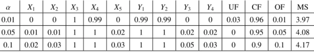
Table 3: Variable selection results for Model 2 based on 1000 repetitions.
α X1 X2 X3 X4 X5 Y1 Y2 Y3 Y4 UF CF OF MS 0.01 0 0 1 0.99 0 0.99 0.99 0 0 0.03 0.96 0.01 3.97 0.05 0.01 0.01 1 1 0.02 1 1 0.02 0.02 0 0.95 0.05 4.08 0.1 0.02 0.03 1 1 0.03 1 1 0.05 0.03 0 0.9 0.1 4.17
The variable selection results for Model 1 is summarized in Table 2. We fixα=0.05 and taken∈ {100,300,700}. We see that the variable selection performance improves asnincreases. Forn=300 andn =700, the unimportant variablesX3,X4,X5,Y1andY2are selected with very low frequencies; the important variablesX1,X2,Y3andY4are selected with frequency 1 or frequency close to 1; and the average model size is close to 4. We also note that the frequency of correctly-fitted model becomes close to 1−αwithn=700.
Table 3 summarizes the variable selection results for Model 2. We fixn=300 and considerα∈ {0.01,0.05,0.1}. Our backward algorithm works well at all nominal levels. The important variablesX3,X4,Y1andY2are selected with high frequencies, the unimportant variablesX1,X2,X5,Y3andY4are selected with low frequencies, and the average model size is close to 4. As expected,α=0.01 leads to smaller models andα=0.1 tend to result in larger models. Again, the frequency of correctly-fitted model is close to 1−α.
5.2. Real data analysis
Beta-carotene and retinol are well studied chemical compounds in the human plasma. Several studies suggest that low levels of both compounds in plasma are associated with increased risk of an array of diseases such as cancer, cardiovascular disease, and cataracts. To determine the role of dietary habits and other health related metrics in plasma concentrations of beta-carotene and retinol, [15] did a cross-sectional study with 12 personal characteristics and dietary metrics for 315 patients with nonmelanoma skin cancer. After removing three categorical variables, we considerx=(X1, . . . ,X9)⊤. The response variables arey =(Y1,Y2)⊤, whereY1is the plasma concentration of beta-carotene andY2 is the plasma concentration of retinol. After exploratory data analysis, we remove six observations with extreme values and getn=309. We apply our proposed dual variable selection procedure from Section 4.4 with significance levelα=0.05, and end up with ˆA={1,2,6,8}and ˆB={1,2}. This suggests that to further study the multivariate associations between dietary habits and the plasma compound concentrations, we can focus only on six variablesX1,X2,X6,X8,Y1andY2instead of the originalxandy.
To demonstrate the effect of variable selection on canonical correlation analysis, we first calculate the first two pairs of canonical covariates (u1,v1) and (u2,v2) based on the original data, wherex ∈ R9 andy ∈ R2. Then we calculate the first two pairs of canonical covariates ( ˜u1,v1) and ( ˜˜ u2,v2) based on the reduced data, where˜ xAˆ ∈ R4 andxBˆ ∈R2. The plots of the canonical covariate from the original data versus the corresponding canonical covariate from the reduced data are provided in Figure 1. The scatterplots are close to the dotted 45 degree line, suggesting that the canonical covariates before and after the data reduction largely agree with each other. This implies that the reduced data keeps the canonical information from the original data.
6. Concluding remarks
In this paper, we propose the CCA-based trace test for the dual marginal coordinate hypotheses and study the asymptotic properties of the resulting test statistic. The validity of the asymptotic test is justified through simulation studies. Based on this novel test, we design a joint backward selection algorithm for dual model-free variable selection.
−4 −2 0 2 4 −4 −2 0 2 4 u ~
1 from reduced data
u1
from orginal data
−6 −4 −2 0 2 4 −6 −4 −2 0 2 4 v ~
1 from reduced data
v1
from orginal data
−2 0 2 4 −2 0 2 4 u ~
2 from reduced data
u2
from orginal data
−6 −4 −2 0 2 −6 −4 −2 0 2 v ~
2 from reduced data
v2
from orginal data
Figure 1. Scatterplots of the canonical covariates from the original data versus the canonical covariate from the reduced data.
The finite-sample performance of the proposed test and the variable selection algorithm are very promising. The dual variable selection and feature screening in the case of divergingpandqis worth future investigation.
Appendix
Proof of Proposition 1. The proof is similar to Proposition 1 in Iaci et al. [8], and is thus omitted. ✷
Proof of Proposition 2. For part (i), note that Span(M)=Span{E(zw⊤)}. Plug inz=Σx−1/2xandw=Σ−y1/2y, and all we need to prove becomes
Span{Σ−x1E(xy⊤)}=Span{Σ− 1/2
x E(zw⊤)} ⊆ Sy|x=Span(β). (A.1)
From the law of iterated expectations and the fact thaty⊥⊥x|β⊤x, we have
E(xy⊤)=E{xE⊤(y|x)}=E{xE⊤(y|β⊤x)}. (A.2) From the property of conditional expectation and the assumption that E(x|β⊤x) is linear inβ⊤x, we have
(A.2) and (A.3) together lead to
Σ−x1E(xy⊤)=β(β⊤Σxβ)−1β⊤E(xy⊤). (A.4) (A.1) follows from (A.4) and proof of part (i) is done. Proof of part (ii) is similar to the proof of part (i), and is thus
omitted. ✷
Proof of Proposition 3. For part (i), assumexF ∈Rp1andx
Fc ∈Rp2withp1+p2 =p. Letx=(x⊤ F,x⊤Fc)⊤. DefineC andDas C= ( Ip1 0 −E(xFcx⊤ F)Σ− 1 xF Ip2 ) and D= ( ΣxF 0 0 ΣxFc|xF ) . ThenCx=(x⊤ F,γ⊤xFc|xF)
⊤,CΣxC⊤=DandΣ−x1=C⊤D−1C. It follows that tr(M)=tr{Σ−1 x E(xy⊤)Σ− 1 y E(yx⊤) } =tr{C⊤D−1CE(xy⊤)Σ−1 y E(yx⊤) } =tr {( Σ−xF1 0 0 Σ−x1 Fc|xF ) ( E(xFy⊤) E(γxFc|xFy⊤) ) Σ−y1 ( E(yx⊤F),E(yγ⊤x Fc|xF) )} =tr Σ −1
xFE(xFy⊤)Σ−y1E(yx⊤F) Σx−F1E(xFy⊤)Σy−1E(yγ⊤xFc|xF)
Σ−xF1c|xFE(γxFc|xFy ⊤)Σ−1 y E(yx⊤F) Σ− 1 xFc|xFE(γxFc|xFy ⊤)Σ−1 y E(yγ⊤xFc|xF) =tr{Σ−x1 FE(xFy ⊤)Σ−1 y E(yx⊤F)}+tr{Σ− 1 xFc|xFE(γxFc|xFy⊤)Σ− 1 y E(yγ⊤xFc|xF)}. Together with tr(MF)=tr{Σ−x1 FE(xFy ⊤)Σ−1 y E(yx⊤F)}, we get δ−F =tr(M)−tr(M F)=tr{Σ−xF1c|xFE(γxFc|xFy ⊤)}Σ−1 y E(yγ⊤xFc|xF)}. (A.5)
For part (ii), the assumption that E(xFc|xF) is a linear function ofxF implies E(xFc|xF)=E(xFcx⊤
F)Σ− 1 xFxF. It follows that E{E(xFcx⊤ F)Σ− 1 xFxFy ⊤}=E{E(x Fc|xF)y⊤}=E{xFcE⊤(y|xF)}. (A.6)
UnderH0F :y⊥⊥x|xF, we have E(y|x)=E(y|xF). Thus
E{xFcE⊤(y|xF)}=E{xFcE⊤(y|x)}=E(xFcy⊤). (A.7)
The definitionγxFc|xF =xFc −E(xFcx⊤F)Σ−
1
xFxF together with (A.6) and (A.7) leads to E(γxFc|xFy⊤)= 0. It follows
from part (i) thatδ−F =0 underHF
0 . ✷
Proof of Proposition 4. The proof is similar to the proof of Proposition 3, and is thus omitted. ✷
Proof of Proposition 5. For part (i), assumeyG ∈Rq1 andy
Gc ∈Rq2withq1+q2=q. Lety=(y⊤ G,y⊤Gc)⊤. DefineK andOas K= ( Iq1 0 −E(yGcy⊤ G)Σ− 1 yG Iq2 ) andO= ( ΣyG 0 0 ΣyGc|yG ) . 10
ThenKy=(y⊤ G,γ⊤yGc|yG)⊤,KΣyK⊤=OandΣ−y1=K⊤O−1K. Thus tr(MF)=tr{Σ−x1 FE(xFy ⊤)Σ−1 y E(yx⊤F) } =tr{Σ−x1 FE(xy ⊤)K⊤O−1K E(yx⊤)} =tr { Σ−xF1 ( E(xFy⊤G),E(xFγ⊤y Gc|yG) ) (Σ−1 yG 0 0 Σ−y1 Gc|yG ) ( E(yGx⊤ F) E(γyGc|yGx⊤F) )} =tr{Σ−x1 FE(xFy ⊤ G)Σ− 1 yGE(yGx⊤F)}+tr{Σ− 1 xFE(xFγ⊤yGc|yG)Σ −1 yGc|yGE(γyGc|yGx⊤F)} =tr(MG F)+tr{Σ− 1 yGc|yGE(γyGc|yGx ⊤ F)Σ− 1 xFE(xFγ ⊤ yGc|yG)}.
Together with (A.5) from the proof of Proposition 3, we get the desired result in part (i). For part (ii), we have seen thaty⊥⊥x |xF leads to E(γx
Fc|xFy
⊤) =0from the proof of Proposition 3. Following similar steps, we can show thaty⊥⊥x | yG leads to E(γyGc|yGx⊤F) = 0. It follows from part (i) thatδ−G−F = 0 under
H0F,[G]:y⊥⊥x|xF andy⊥⊥x|yG. ✷
We need Lemma 1 and Lemma 2 before we prove Theorem 1. Let ¯xF = n−1∑n
i=1x (i) F, ˜x (i) F = x (i) F −x¯F, and ˆ ΣxF = n− 1∑n i=1x˜ (i) F(˜x (i) F)⊤. Similarly we define ˜y (i) and ˜x(i) Fc. Let En(xFx⊤Fc) = n− 1∑n i=1x˜ (i) F(˜x (i) Fc)⊤, ˆγ (i) xFc|xF = x˜(i) Fc − En(xFcx⊤ F) ˆΣ −1 xFx˜ (i) F, and En(yγˆ⊤xFc|xF)=n− 1∑n i=1y˜ (i) ( ˆγ(xi) Fc|xF) ⊤. Define Π(i) ={y˜(i)−E(yx⊤ F)Σ− 1 xFx˜ (i) F } { (˜x(i) Fc)⊤−(˜x (i) F)⊤Σ− 1 xFE(xFx⊤Fc) }
and we have the following result.
Lemma 1. SupposeE(x)=0,E(y)=0, andE(x
Fc|xF)is a linear function ofxF. Ify⊥⊥x|xF, then
En(yγˆ⊤xFc|xF)= 1 n n ∑ i=1 Π(i)+Op(n−1), where the first term on the right-hand side is of order Op(n−1/2).
Proof of Lemma 1. From the definition of ˆγxFc|xF andγxFc|xF, we have En(yγˆ⊤xFc|xF)−E(yγ⊤xFc|xF)={En(yx⊤Fc)−E(yx⊤Fc)} −[En{yx⊤FΣˆ−
1 xFEn(xFx ⊤ Fc)} −E{yx⊤FΣ− 1 xFE(xFx ⊤ Fc)}]. (A.8)
Because E(x)=0and E(y)=0, it can be shown that
En(yx⊤Fc)−E(yx⊤Fc)= 1 n n ∑ i=1 {y˜(i)(˜x(i) Fc)⊤−E(yx⊤Fc)}+Op(n−1). (A.9)
The asymptotic expansions of ˆΣ−xF1and En(xFx
⊤ Fc) are, respectively, ˆ Σ−xF1−Σ −1 xF =−Σ −1 xF 1n n ∑ i=1 { ˜ x(i) F(˜x (i) F)⊤−ΣxF } Σ−xF1+Op(n −1 ) and (A.10) En(xFx⊤Fc)−E(xFx⊤Fc)= 1 n n ∑ i=1 { ˜ x(i) F(˜x (i) Fc)⊤−E(xFx⊤Fc) } +Op(n−1). (A.11)
Eqs. (A.10) and (A.11) together lead to ˆ Σ−xF1En(xFx⊤Fc)−Σ− 1 xFE(xFx⊤Fc)= 1 n n ∑ i=1 Σ−xF1x˜ (i) F { (˜x(i) Fc)⊤−(˜x (i) F)⊤Σ− 1 xFE(xFx⊤Fc) } +Op(n−1). (A.12) It follows from (A.12) that
En{yx⊤FΣˆ− 1 xFEn(xFx⊤Fc)} −E{yx⊤FΣ−xF1E(xFx⊤Fc)}= 1 n n ∑ i=1 E(yx⊤F)Σ−xF1x˜ (i) F { (˜x(i) Fc)⊤−(˜x (i) F)⊤Σ− 1 xFE(xFx⊤Fc) } +1 n n ∑ i=1 {y˜(i)(˜x(i)
F)⊤−E(yx⊤Fc)}Σ−xF1E(xFx⊤Fc)+Op(n−1). (A.13)
Eqs. (A.8), (A.9) and (A.13) together lead to
En(yγˆ⊤xFc|xF)=En(yx ⊤ Fc)−En{yx⊤FΣˆ− 1 xFEn(xFx⊤Fc)}= 1 n n ∑ i=1 [ ˜ y(i)(˜x(i) Fc)⊤−y˜ (i) (˜x(i) F)⊤Σ− 1 xFE(xFx⊤Fc) −E(yx⊤F)Σ−xF1x˜ (i) F { (˜x(i) Fc)⊤−(˜x (i) F)⊤Σ− 1 xFE(xFx ⊤ Fc) }] +Op(n−1) =1 n n ∑ i=1 { ˜ y(i)−E(yx⊤F)Σ−xF1x˜ (i) F } { (˜x(i) Fc)⊤−(˜x (i) F)⊤Σ− 1 xFE(xFx⊤Fc) } +Op(n−1), (A.14)
which is the desired result. ✷
Similarly, let En(yGy⊤Gc)=n− 1∑n i=1y˜ (i) G(˜y (i) Gc)⊤, ˆγ (i) yGc|yG =y˜(i) Gc−En(yGcy⊤ G) ˆΣ −1 yGy˜ (i) G, and En(xFγˆ⊤yGc|yG)=n− 1∑n i=1x˜ (i) F( ˆγ (i) yGc|yG) ⊤. Define Λ(i)={x˜(i) F −E(xFy⊤G)Σ− 1 yGy˜ (i) G } { (˜y(i) Gc)⊤−(˜y (i) G)⊤Σ− 1 yGE(yGy⊤Gc) } and we have
Lemma 2. SupposeE(x)=0,E(y)=0, andE(y
Gc|yG)is a linear function ofyG. Ify⊥⊥x|yG, then
En(xFγˆ⊤yGc|yG)= 1 n n ∑ i=1 Λ(i)+Op(n−1), where the first term on the right-hand side is of order Op(n−1/2).
Proof of Lemma 2. The proof is similar to the proof of Lemma 1, and is thus omitted. ✷
Proof of Theorem 1. Recall that |F | = p1, |Fc
| = p2, |G| = q1, |Gc | = q2, p1 +p2 = p and q1 +q2 = q. Letϕ1 = vec{Σ− 1/2 y E(yγ⊤xFc|xF)Σ− 1/2 xFc|xF} ∈ Rqp2, ϕ 2 = vec{Σ− 1/2 xF E(xFγ⊤yGc|yG)Σ− 1/2 yGc|yG} ∈ Rp1q2, and ψ = (ϕ⊤ 1,ϕ⊤2)⊤, where vec denotes vectorization. Then we have δ−G
−F = ψ⊤ψ. At the sample level, let ˆψ = ( ˆϕ ⊤ 1,ϕˆ ⊤ 2)⊤, where ˆ ϕ1=vec{Σˆ−1/2 y En(yγˆ⊤x Fc|xF) ˆΣ −1/2 xFc|xF}and ˆϕ2=vec{Σˆ −1/2 xF En(xFγˆ ⊤ yGc|yG) ˆΣ −1/2 yGc|yG}. Then we have ˆ δ−G −F =ψˆ ⊤ψˆ. (A.15) UnderH0F,[G], we havey⊥⊥x|xF. It follows that E(yγ⊤
xFc|xF)=0andϕ1=0. Together with Lemma 1, we have ˆ ϕ1= 1 n n ∑ i=1 vec{Σ−y1/2Π(i)Σ− 1/2 xFc|xF} +Op(n−1), (A.16) 12
where the first term on the right-hand side is of orderOp(n−1/2). Similarly, we havey⊥⊥x|yGunderH0F,[G]. It follows that E(xFγ⊤
yGc|yG)=0andϕ2 =0. Together with Lemma 2, we have ˆ ϕ2= 1 n n ∑ i=1 vec{Σ−xF1/2Λ(i)Σ− 1/2 yGc|yG}+Op(n−1), (A.17)
where the first term on the right-hand side is of orderOp(n−1/2). It follows from (A.16) and (A.17) that
ˆ ψ= 1 n n ∑ i=1 ϑ(i)+Op(n−1), (A.18) where ϑ(i) = { vec⊤(Σ−y1/2Π(i)Σ− 1/2 xFc|xF),vec⊤(Σ− 1/2 xF Λ(i)Σ− 1/2 yGc|yG) }⊤ ∈RL with E(ϑ(i))=0andL=qp2+p1q2=pq−p1q1. As a result of (A.18), we have
√
nψˆ N(0,Ω) (A.19)
asn→ ∞, whereΩ=E{ϑ(i)(ϑ(i))⊤}. Eqs. (A.19) and (A.15) lead to the desired result. ✷ As a special case,δ−G
−F reduces toδ−F when we setG=Iy. Thenδ−F =ϕ1⊤ϕ1and ˆδ−F =ϕˆ⊤1ϕˆ1. It follows from (A.16) that ˆϕ1 =n−1 ∑n i=1ϑ (i) 1 +Op(n−1), whereϑ (i) 1 =vec{Σ− 1/2 y Π(i)Σ− 1/2 xFc|xF} ∈ Rp2q. Thus √nϕˆ 1 N(0,Γ), where Γ=E{ϑ(i) 1(ϑ (i)
1 )⊤}. The asymptotic distribution of ˆδ−F is summarized in the next result. Corollary 1. SupposeE(x)=0,E(y)=0, andE(x
Fc|xF)is a linear function ofxF. Then underH0F :y⊥⊥x|xF,
nδˆ−F
p2q
∑
ℓ=1
ρℓχ2ℓ(1)
as n→ ∞, whereχ2ℓ(1)is independent chi-square with one degree of freedom forℓ∈ {1, . . . ,p2q}, andρ1≥ · · · ≥ρp2q are the eigenvalues ofΓ.
Similarly,δ−G
−F becomesδ−Gwhen we setF =Ix. Note thatδ−G=ϕ⊤3ϕ3withϕ3=vec{Σ− 1/2
x E(xγ⊤yGc|yG)Σ
−1/2 yGc|yG} ∈
Rpq2, and ˆδ−G = ϕˆ⊤3ϕˆ3 with ˆϕ3 = vec{Σˆ−x1/2En(xγˆ⊤ yGc|yG) ˆΣ
−1/2
yGc|yG}. Similar to (A.17), it can be shown that ˆϕ3 = n−1∑ni=1ϑ (i) 3 +Op(n− 1 ), whereϑ(3i) =vec{Σx−1/2Λ(i)Σ−1/2 yGc|yG}. Thus √nϕˆ 3 N(0,Υ), whereΥ =E{ϑ (i) 3(ϑ (i) 3 )⊤}. The asymptotic distribution of ˆδ−Gis summarized in the next result.
Corollary 2. SupposeE(x)=0,E(y)=0, andE(yGc|yG)is a linear function ofyG. Then underH[G]
0 :y⊥⊥x|yG, nδˆ−G pq2 ∑ ℓ=1 ωℓχ2ℓ(1) as n→ ∞, whereχ2
ℓ(1)is independent chi-square with one degree of freedom forℓ∈ {1, . . . ,pq2}, andω1≥ · · · ≥ωpq2 are the eigenvalues ofΥ.
Derivation ofBfor Model 1. Let
Σϵ = 1 .5 .25 .125 .5 1 .5 .25 .25 .5 1 .5 .125 .25 .5 1 and H= 0 0 0 0 0 0 0 0 0 0 0 0 0 0 0 1 1 0 0 0 .
Becausey=Hx+ϵ, we have Σy=HΣxH⊤+Σϵ = 1 .5 .25 .125 .5 1 .5 .25 .25 .5 1 .5 .125 .25 .5 3 and Σ−y1= 4/3 −2/3 0 0 −2/3 5/3 −2/3 0 0 −2/3 47/33 −2/11 0 0 −2/11 4/11 . It follows that E(x|y)=ΣxyΣ−1 y y= 0 0 0 1 0 0 0 1 0 0 0 0 0 0 0 0 0 0 0 0 4/3 −2/3 0 0 −2/3 5/3 −2/3 0 0 −2/3 47/33 −2/11 0 0 −2/11 4/11 Y1 Y2 Y3 Y4 = 2 11 2Y4−Y3 2Y4−Y3 0 0 0 .
Thus we haveB={3,4}for Model 1. ✷
References
[1] E. Cand`es, T. Tao, The Dantzig selector: Statistical estimation whenpis much larger thann, Ann. Statist. 35 (2007) 2313–2351. [2] R.D. Cook, Regression Graphics: Ideas for Studying Regressions through Graphics, Wiley, New York, 1998.
[3] R.D. Cook, Testing predictor contributions in sufficient dimension reduction, Ann. Statist. 32 (2004) 1062–1092.
[4] R.D. Cook, S. Weisberg, Discussion of “sliced inverse regression for dimension reduction” by K.C. Li, J. Amer. Statist. Assoc. 86 (2004) 328–332.
[5] J. Fan, R. Li, Variable selection via nonconcave penalized likelihood and its oracle properties, J. Amer. Statist. Assoc. 96 (2001) 1348–1360. [6] H. Hotelling, Relations between two sets of variables. Biometrika 58 (1936) 433–451.
[7] J. Huang, J.L. Horowitz, F. Wei, Variable selection in nonparametric additive models, Ann. Statist. 38 (2010) 2282–2313. [8] R. Iaci, X. Yin, L.X. Zhu, The dual central subspaces in dimension reduction, J. Multivariate Anal. 145 (2016) 178–189. [9] B. Jiang, J. Liu, Variable selection for general index models via sliced inverse regression, Ann. Statist. 42 (2014) 1751–1786. [10] B. Li, S. Wang, On directional regression for dimension reduction, J. Amer. Statist. Assoc. 102 (2007) 997–1008.
[11] K.C. Li, Sliced inverse regression for dimension reduction (with discussion), J. Amer. Statist. Assoc. 86 (1991) 316–342. [12] L. Li, Sparse sufficient dimension reduction, Biometrika 94 (2007) 603–613.
[13] L. Li, R.D. Cook, C.J. Nachtsheim, Model-free variable selection, J. R. Stat. Soc. Ser. B 67 (2005) 285–299.
[14] J.Y. Liu, R. Li, R. Wu, Feature selection for varying coefficient models with ultrahigh dimensional covariates, J. Amer. Statist. Assoc. 109 (2014) 266–274.
[15] D.W. Nierenberg, T.A. Stukel, J.A. Baron, B.J. Dain, E.R. Greenberg, S.C.P.S. Group, Determinants of plasma levels of beta-carotene and retinol, Amer. J. Epidemiol. 130 (1989) 511–521.
[16] Y. Shao, R.D. Cook, S. Weisberg, Mariginal tests with sliced average variance estimation, Biometrika 94 (2007) 285–296. [17] R.J. Tibshirani, Regression shrinkage and selection via the lasso, J. R. Stat. Soc. Ser. B 58 (1996) 267–288.
[18] L. Wang, L. Xue, A. Qu, H. Liang, Estimation and model selection in generalized additive partial linear models for correlated data with diverging number of covariates, Ann. Statist. 42 (2014) 592–624.
[19] Z. Yu, Y. Dong. Model-free coordinate test and variable selection via directional regression, Statist. Sinica 26 (2016) 1159–1174.
[20] Z. Yu, Y. Dong, Y. Fang, Marginal coordinate tests for central mean subspace with principal hessian directions, Chinese J. Appl. Probab. Statist. 26 (2010) 544–552.
[21] Z. Yu, Y. Dong, L.X. Zhu, Trace pursuit: A general framework for model-free variable selection, J. Amer. Statist. Assoc. 111 (2016) 813–821. [22] H. Zou, The adaptive lasso and its oracle properties, J. Amer. Statist. Assoc. 101 (2006) 1418–1429.