Assessing CoDa regression for modelling daily multivariate air pollutants evolution

Assessing CoDa regression for modelling daily multivariate air

pollutants evolution

Joseph Sánchez-Balseca1_{, Agustí Pérez-Foguet}1 1_{Engineering Sciences and Global Development (EscGD),}

Civil and Environmental Engineering Department, Universitat Politècnica de Catalunya, Barcelona, Spain.

[email protected] Summary

The application of the theory of compositional data in multivariate spatio-temporal statistical models is still scarce, even though the results obtained are robust. Actually, this kind of models are attractive to pollution model developers, due to, its versatility in the spatio-temporal variables; but nobody has tried to use it with compositional data yet. The main differences between a conventional model and two CoDa models (with two sequential binary partition, SBP) were analyzed. The first SBP was proposed by pollutants relationship interpretation, and the second one was imposed as standard SBP (R studio). Initially the conventional temporal model is used to predicting pollution levels to fill missing data or predicting pollution levels on future days. The application of compositional data theory in conventional temporal air quality models allowed to obtain acceptable quality models, whose results were adjusted to the observed values. Nash-Sutcliffe Efficiency Index (NSE) and root-mean-square error (RMSE), were used to evaluating the model quality and fitted values respectively.

Key words: air quality, compositional data, SBP, multivariate response model, precision.

1

Introduction

Predictions from numerical models are also used for environmental regulatory purposes and improved decision-making strategies (Zannetti, 1990; Mayer 1999; Dominici et al. 2002; Cetin et al. 2017; Paci, 2013). Shaddick G. et al. (2002) studied the hierarchical Dynamic Linear Model (DLM) applied to four pollutants, at eight monitor stations. Gutierrez et al. (2016), proposed to model the measurements of particulate matter, by means of a Bayesian nonparametric dynamic model. Recently, Shaddick et al. (2018), developed a spatially-varying model, within a Bayesian hierarchical modelling framework.

Most data in the geo-environmental sciences are compositional in character. They describe quantitatively the parts of a whole. If concentrations are not considered as compositional data, incorrect conclusions could be obtained (Egozcue and

Pawlowsky-Glahn, 2011). Due to the advances in the compositional data analysis since 2000, the statistical works can be resolved in three steps: data transformations to log-ratio coordinates, traditional statistical analysis with the coordinates, and finally result analysis (Aitchison et al., 2002; Egozcue et al., 2003; van den Boogaart and Tolosana, 2013).

The present work has been structured as: Methodology (section 2), Results (section 3), and Conclusions (section 4).

2

Methodology

The methodology will begin with a data description, then it will explain the hierarchical Dynamic Linear Model theory, the compositional data concepts used, and finally a numerical comparison analysis (models).

2.1

Data

The data used in the temporal multivariate linear models was collected hourly over the period 2009-2013, from three air quality monitoring stations at Quito-Ecuador (Environmental Department of Quito, 2017). The main stations characteristics are showed in the table 1.

Table 1: Main parameter of three monitor stations.

Station Name Location High (mals) Station code

CARAPUNGO 78°26'50'' W, 0°5'54'' S 2660 1

BELISARIO 78°29'24'' W, 0°10'48'' S 2835 2

EL CAMAL 78°30'36'' W, 0°15'00'' S 2840 3

This tree station covering the urban Quito territory, and are located in the north (CARAPUNGO/Station Nº 1), in the center (BELISARIO/Station Nº 2), and south (EL CAMAL/Station Nº 3); as it is showed in the figure 1.

The data analyzed as dependent variable were carbon monoxide (CO), nitrogen dioxide (NO$), Sulphur dioxide (SO$), and ozone (O&). To obtain the daily mean

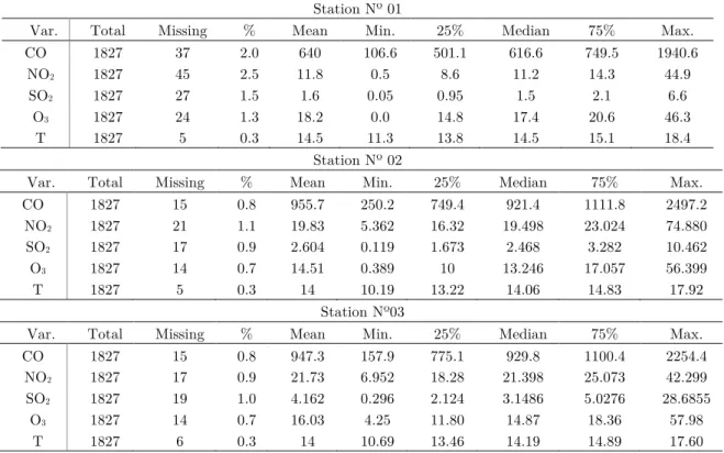
concentration, the presence of 75% hourly data, was imposed. The variable with more missing daily values was nitrogen dioxide (2.5%, 1.1%), at station 1 and 2 respectively. The data description is showed in the table 2, where the units to pollutants are given as parts per billion (ppb), and Kelvin units (K) for temperature.

Table 2: Summary of variables measured at three monitor stations, 2009-2013. Station Nº 01

Var. Total Missing % Mean Min. 25% Median 75% Max.

CO 1827 37 2.0 640 106.6 501.1 616.6 749.5 1940.6 NO2 1827 45 2.5 11.8 0.5 8.6 11.2 14.3 44.9 SO2 1827 27 1.5 1.6 0.05 0.95 1.5 2.1 6.6 O3 1827 24 1.3 18.2 0.0 14.8 17.4 20.6 46.3 T 1827 5 0.3 14.5 11.3 13.8 14.5 15.1 18.4 Station Nº 02

Var. Total Missing % Mean Min. 25% Median 75% Max.

CO 1827 15 0.8 955.7 250.2 749.4 921.4 1111.8 2497.2 NO2 1827 21 1.1 19.83 5.362 16.32 19.498 23.024 74.880 SO2 1827 17 0.9 2.604 0.119 1.673 2.468 3.282 10.462 O3 1827 14 0.7 14.51 0.389 10 13.246 17.057 56.399 T 1827 5 0.3 14 10.19 13.22 14.06 14.83 17.92 Station Nº03

Var. Total Missing % Mean Min. 25% Median 75% Max.

CO 1827 15 0.8 947.3 157.9 775.1 929.8 1100.4 2254.4

NO2 1827 17 0.9 21.73 6.952 18.28 21.398 25.073 42.299

SO2 1827 19 1.0 4.162 0.296 2.124 3.1486 5.0276 28.6855

O3 1827 14 0.7 16.03 4.25 11.80 14.87 18.36 57.98

T 1827 6 0.3 14 10.69 13.46 14.19 14.89 17.60

2.2

Dynamic Linear Models/Temporal air quality model

The most widely known applied subclass is that of normal dynamic linear models, referred as dynamic linear models, or DLMs (West and Harrison, 1997). For this work, Y₍₎ represent the pollutant p concentration, on day t, the observation [Eq. (3)] and system [Eq. (4)] equations respectively are

𝑌

= 𝜃

+ 𝑣

𝑣

~𝑁(0, 𝜎

₎

₍₃₎

𝜃

= 𝜃

+ 𝑤

𝑤

~𝑁(0, 𝜎

₎

The conditional variance 𝜎=$ is not comparable with 𝜎8$. The multiple pollutants at

any time point were modelled as arising from a multivariate Gaussian random field. 𝑣, represents the measurement errors which are assumed to be independent

and identically distributed 𝑁 0, 𝜎₈₊$ _{; 𝑤}

, to each pollutant are independent and

identically distributed multivariate normal random variables with zero mean and variance-covariance matrix Σ+. To this work a Bayesian approach was adopted,

with prior distribution being assigned to the unknown parameters and missing observations. Gamma priors are proposed for the precisions 𝜎8:$~𝐺𝑎 𝑎8, 𝑏8 , in the

multivariate updating scenario, the variance-covariance matrix Σ₊:;_~𝑊

+ 𝐷, 𝑑 , where 𝑊+ 𝐷, 𝑑 denotes a P-dimensional Wishart distribution with

mean D and precision parameter d.

2.3

Compositional Data

In mathematical terms, compositional data are represented [Eq. (6)] as pertaining to a sample space called the simplex 𝑆F

𝑆

_{= 𝑥 = 𝑥}

;

, 𝑥

, 𝑥

: 𝑥

> 0 𝑖 = 1,2, 𝐷 ,

𝑋

= 𝐾

where K is a given positive constant, defined a priori and depending on how the parts are measured (Buccianti, 2013). This work has four gaseous pollutants (ppb), and the composition to be analysed would be 𝐶𝑂, 𝑁𝑂$, 𝑆𝑂$, 𝑂&, 𝑅 , in this case the

residual part was not of interest, for this reason the subcompositional approach is used (the subcomposition closure for each day is saved to be used in the model evaluation). The subcompositional incoherence, was eliminated through log-ratio methods (Buccianti et al., 2006). Aitchison (1982) developed the additive–log-ratio (alr) and centred-log-ratio (clr) transformations; Egozcue et al. (2003) introduced the isometric-log-ratio (ilr) transformation.

The isometric-log ratio (ilr) transformation, was used. In this framework, the procedure of the sequential binary partition (SBP) to identify orthonormal coordinates was adopted (Egozcue and Pawlowsky-Glahn, 2005). For this study, the standard base (function in R-studio) and SBP method [Eq. (6)] were used. Considering the four pollutants as sub composition (𝑋𝐶𝑂, 𝑋𝑁𝑂$, X𝑆𝑂$, X𝑂&), in first

level, the group was divided as: 𝑆𝑂_$, 𝑂_& and 𝐶𝑂, 𝑁𝑂_$. One group is related by patterns that showed air pollutant pairs of O3/SO2 appearing at the same hour of the day (Meagher et al., 1827; EPA, 2001).

𝑥

₌

𝑙𝑛

𝑥

₌

𝑙𝑛

𝑥

₌

𝑙𝑛

2.4

Comparison Models

To evaluating and comparing the models, Nash-Sutcliffe Efficiency Index (NSE) and root-mean-square error (RMSE), were used. NSE is a widely used and potentially reliable statistic for assessing the goodness of fit of hydrologic models.

The NSE scale is from 0 to 1 [Eq. (8)], NSE = 1 means the model is perfect. NSE = 0 means that the model is equal to the average of the observed data, and negative values mean that the average is a better predictor (McCuen et al., 2006).

𝑁𝑆𝐸 = 1 −

defgh:defg ^ (8)

Root Mean Square Error (RMSE) is a measure of quantitative performance commonly used to evaluate demand forecasting methods. The lower RMSE, it means that the model has no error [Eq. (9)].

𝑅𝑀𝑆𝐸 =

m (9)

3

Results

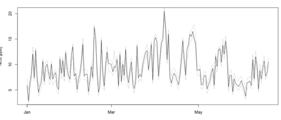
The conventional model for nitrogen dioxide presented adequate fitted values; in the station 1, it presented the less variability value, and its behavior for a subset of recorded measurements (90% confidence interval band) and estimated q for station 1 is showed in the figure 2.

Figure 2: Conventional temporal model (year: 2011; 90% confidence interval) Threshold value suggested to indicate a model of sufficient quality is NSE>0.5 (Ritter and Muñoz-Carpena, 2013). In general, the conventional model had low NSE values. If threshold value is used, the models to evaluating the behavior of CO at station 1 (NSE=0.43), and SO2 at station 3 (NSE=0.45) have not sufficient quality. In comparison with the compositional models, which had NSE values over the threshold for all pollutants (NSE≥0.62).

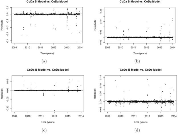
In general, a lower RMSE is better than a higher one. If RMSE is zero, the model has perfect fit to the data. The RMSE values for conventional model were high, except to SO2 at stations 1 and 2. The compositional model (RMSE ≤ 0.009) presented a better fitted data for all pollutants. For this work, two SBP were used, therefore similar results were obtained, the littles differences found among them are showed in the figure 3, where the residuals of CO and NO2 had higher values than SO2 and O3. These differences were generated in the error treatment over transformations.

The two compositional models presented acceptable fitted values, more than conventional model. The NSE and RMSE mean values are showed in the table 8.

(a) (b)

(c) (d)

Figure 3: Residuals between compositional models for station 1: (a) CO, (b) NO2, (c) SO2, and (d) O3

Table 8: NSE and RMSE mean values for each model.

Model Compositional model

(standard base)

Compositional model (base imposed)

STATION NSE RMSE NSE RMSE NSE RMSE

1 0,6867009 39,04213233 0,759960075 0,004501534 0,929408425 0,002467467 2 0,79693 33,47364475 0,924419225 0,002468459 0,952827725 0,001662221

3 0,681427375 3,118657 0,981204225 0,001408042 0,84546585 0,004259196

MEAN 0,721686092 25,21147803 0,888527842 0,002792679 0,909234 0,002796295

4

Conclusions

The compositional data concepts applied to temporal models (Dynamic Linear Models) presented good results, like as better-quality models and better fitted values. These results are due to use the air pollutants concentrations as compositions. Compositional models had less variability than conventional models, over all pollutants at three stations.

Acknowledgements and appendices

The authors would like to thank the “Secretaría Nacional de Educación Superior, Ciencia, Tecnología e Innovación de la República del Ecuador” for financial support.

References

Aitchison, J. 1982. «The statistical analysis of compositional data (with discussion)». Journal of the Royal Statistical Society 139-177.

Aitchison, J., Barceló-Vidal, C., J.J. Egozcue, y V. Pawlowsky- Glahn. 2002. «A concise guide for the algebraic-geomet- ric structure of the simplex, the sample space for compo- sitional data analysis». The eighth annual con- ference of the international Association for Mathematical Geology, Volume I and II. Berlín: Selbstverlag der Alfred-Wegener-Stiftung. 387-392.

Akpinar, Ebru, Sinan Akpinar, y Hakan Öztop. 2009. «Statistical analysis of meteorological factors and air pollution at winter months in Elaziğ, Turkey.» Journal of Urban and Environmental 7-16.

Buccianti, A., G. Mateu, y V. Pawlowsky. 2006. Compositional Data Analysis in the Geosciences. London: Geological Society.

Buccianti, Antonella. 2013. «Is compositional data analysis a way to see beyond the illusion?» Computers y Geosciences 165-173.

Dominici, Francesa, Aidan McDermott, Scott Zeger, y Jonathan Samet. 2002. «On the Use of Generalized Additive Models in Time-Series Studies of Air Pollution and Health.» American Journal of Epidemiology 193–203.

Egozcue, J. J., y V. Pawlowsky-Glahn. 2011. «Análisis composicional de datos en Ciencias Geoambientales.» Boletín Geológico y Minero 439-452.

Egozcue, J., y V. Pawlowsky-Glahn. 2005. «Groups of parts and their balances in compositional data analysis.» Mathematical Geology 795-828.

Egozcue, J.J., V. Pawlowsky-Glahn, G. Mateu-Figueras, y C. Barceló-Vidal. 2003. «Isometric logratio transformations for compositional data analysis.» Mathematical Geology 279-300.

Egozcue, Juan José, Josep Daunis-i-Estadella, Vera Pawlowsky-Glahn, Karel Hron, y Peter Filzmoser. 2012. «Simplicial regression. The normal model.» Journal of Applied Probability and Statistics 87-108.

Environmental Protection Agency. 2001. AQS . Report, Washington: EPA.

Gutiérrez, Luis, Ramsés H. Mena, y Matteo Ruggiero. 2016. «A time dependent Bayesian nonparametric model for air quality analysis.» Computational Statistics and Data Analysis 161–175.

Marinov, Marin, Ivan Tapalov, Elitsa Gieva, y Georgi. Nicolov. 2016. «Air quality monitoring in urban environments.» 2016 39th International Spring Seminar on Electronics Technology (ISSE). Pilsen: IEEE. 443 - 448.

Mayer, Helmut. 1999. «Air pollution in cities.» Atmospheric Environment 4029-4037.

McCuen, Richard H., Zachary Knight, y A. Gillian Cutter. 2006. «Evaluation of the Nash–Sutcliffe Efficiency Index.» Journal of Hydrologic Engineering.

the southeastern United States. .» Atmospheric Environment 605–615.

Paci, Lucia. 2013. Bayesian space-time data fusion for real-time forecasting and map uncertainty. Bologna: Università di Bologna.

Ritter, Axel, y Rafael Muñoz-Carpena. 2013. «Performance evaluation of hydrological models: Statistical significance for reducing subjectivity in goodness-of-fit assessments.» Journal of Hydrology 33-45.

Sarstedt, M., y E. Mooi. 2014. «A Concise Guide to Market Research.» Business and Economics 273-324.

Secretaria de Medio Ambiente DMQ. 2017. Informe de Calidad del Aire DMQ 2017. Quito: Distrito Metropolitano de Quito.

Shaddick, Gavin, Matthew L. Thomas, Amelia Jobling, Michael Brauer, Aaron van Donkelaar, Rick Burnett, Howard Chang, y otros. 2018. «Data integration model for air quality: a hierarchical approach to the global estimation of exposures to ambient air pollution.» Royal Statistical Society 231–253.

Shaddick, Gavin, y Jon Wakefield. 2002. «Modelling Daily Multivariate Pollutant Data at Multiple Sites.» Journal of the Royal Statistical Society (Wiley) 351-372.

Tolosana, R., y H. Eynatten. 2010. «Simplifying compositional multiple regression: Application to grain size controls on sediment geochemistry.» Computers & Geosciences 577-589.

van den Boogaart, K. Gerald, y Raimon Tolosana-Delgado. 2013. Analyzing Compositional Data with R. Berlin: Springer.

West, Mike, y Jeff Harrison. 1997. Bayesian Forecasting and Dynamic Models. New York: Springer-Verlag.

Zannetti, Paolo. 1990. Air pollution Modeling . Monrovia, California: Springer Science.